AP/College Calculus AB
Institution: MIT
42 study materials · 11 sections
The Client Challenge course is a comprehensive AP®/College Calculus AB curriculum designed to master the foundational principles of calculus. It covers ten core units ranging from limits and continuity to advanced applications of integration and differential equations. Students engage with conceptual theories, analytical techniques, and real-world problem-solving to prepare for the AP Calculus AB exam and higher-level mathematics.
Course Sections
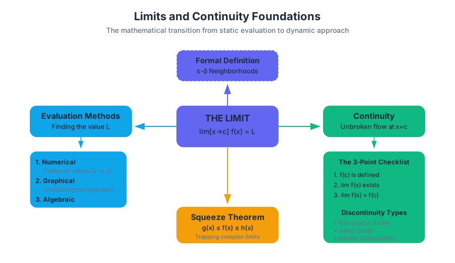
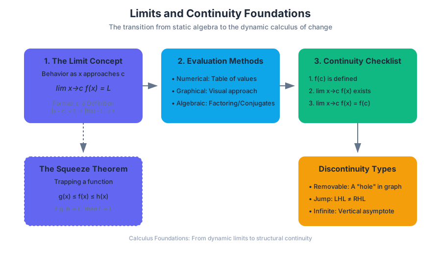
Limits and Continuity Foundations
Key concepts: Limits (Graphical and Algebraic) · Continuity at a Point · Squeeze Theorem · Intermediate Value Theorem (IVT) · Infinite Limits and Asymptotes
Introduction to the concept of limits, defining continuity, and exploring fundamental theorems.
Limits and Continuity Foundations
Calculus is often described as the mathematics of change, but before we can quantify change, we must quantify the "nearness" of values. In classical algebra, we deal with static values: $f(2)$ is exactly some number. In calculus, we ask a more sophisticated question: "As $x$ gets arbitrarily close to 2, what happens to $f(x)$?" This shift from static evaluation to dynamic approach is the birth of the Limit.
The Concept of the Limit
At its core, a limit describes the behavior of a function as its input approaches a specific value. We denote this as:
$$\lim_{x \to c} f(x) = L$$
This statement reads: "The limit of $f(x)$ as $x$ approaches $c$ equals $L$." Crucially, the limit is concerned with the neighborhood of $c$, not the value of $f(c)$ itself. In fact, $f(c)$ might be undefined, yet the limit can still exist.
Formal Definition ($\epsilon$-$\delta$)
To a mathematician, "arbitrarily close" is too vague. The formal definition, provided by Cauchy and Weierstrass, is the $\epsilon$-$\delta$ definition:
The limit of $f(x)$ as $x$ approaches $c$ is $L$ if, for every $\epsilon > 0$, there exists a $\delta > 0$ such that if $0 < |x - c| < \delta$, then $|f(x) - L| < \epsilon$.
This means if you pick a tiny distance $\epsilon$ from the target $L$, I can find a tiny distance $\delta$ around $c$ such that every $x$ in that range (except possibly $c$ itself) maps to a value within $\epsilon$ of $L$.
Graphical and Numerical Estimation
Before diving into algebra, we often estimate limits using two primary methods:
- Numerical Estimation: Creating a table of values that "zoom in" on $c$ from both sides (e.g., 1.9, 1.99, 1.999 and 2.1, 2.01, 2.001).
- Graphical Estimation: Observing the height the graph approaches from the left and right.
| Method | Strengths | Weaknesses |
|---|---|---|
| Numerical | Intuitive, handles complex functions easily with a calculator. | Can be misleading if the function oscillates wildly (e.g., $\sin(1/x)$). |
| Graphical | Excellent for identifying jump discontinuities and asymptotes. | Imprecise; "looks like 2" might actually be 2.0001. |
| Algebraic | Provides exact, provable values. | Can be difficult for transcendental or non-elementary functions. |
Algebraic Evaluation Techniques
When direct substitution ($\text{plugging in } c$) results in an indeterminate form like $0/0$, we employ several strategies:
- Factoring: Canceling out the "problematic" term.
- Rationalization: Using conjugates to clear radicals.
- Simplification: Combining complex fractions.
/*
 * A low-level numerical approximation of a limit in C.
 * This demonstrates the "epsilon-delta" approach by testing
 * values increasingly close to the target 'c'.
 */
#include <stdio.h>
#include <math.h>

double f(double x) {
    // Example: f(x) = (x^2 - 4) / (x - 2)
    // We know the limit as x -> 2 is 4.
    return (pow(x, 2) - 4) / (x - 2);
}

int main() {
    double target = 2.0;
    double epsilon = 0.00000001;
    double delta = 0.1;

    printf("Approaching %f:\n", target);
    for(int i = 0; i < 10; i++) {
        double x_left = target - delta;
        double x_right = target + delta;
        printf("Delta: %.10f | f(left): %.10f | f(right): %.10f\n",
                delta, f(x_left), f(x_right));
        delta /= 10.0; // Zoom in by factor of 10
    }
    return 0;
}
Continuity at a Point
A function is continuous if its graph can be drawn without lifting your pencil. However, in technical terms, continuity is defined by the behavior of limits. Continuity at a point $x = c$ requires three strict conditions to be met.
The Three-Point Checklist
A function $f(x)$ is continuous at $x = c$ if and only if:
- $f(c)$ is defined ($c$ is in the domain).
- $\lim_{x \to c} f(x)$ exists (left-hand limit = right-hand limit).
- $\lim_{x \to c} f(x) = f(c)$ (the limit matches the actual value).
Types of Discontinuity
If any of the three conditions above fail, the function is discontinuous. We classify these failures into three categories:
| Discontinuity Type | Description | Removability |
|---|---|---|
| Removable (Hole) | The limit exists, but $f(c)$ is undefined or different from the limit. | Removable: Can be fixed by redefining a single point. |
| Jump | The left-hand and right-hand limits exist but are not equal. | Non-removable: Common in piecewise functions. |
| Infinite | The function approaches $\pm\infty$ as $x \to c$. | Non-removable: Occurs at vertical asymptotes. |
Continuity on an Interval
A function is continuous on an open interval $(a, b)$ if it is continuous at every point in the interval. For a closed interval $[a, b]$, we also require one-sided continuity at the endpoints:
- $\lim_{x \to a^+} f(x) = f(a)$
- $\lim_{x \to b^-} f(x) = f(b)$
The Squeeze Theorem
Sometimes, a limit is too complex to evaluate directly (e.g., $\lim_{x \to 0} x^2 \sin(1/x)$). The Squeeze Theorem (also known as the Sandwich Theorem) allows us to find the limit of a "difficult" function by trapping it between two "easier" functions.
The Theorem
If $g(x) \le f(x) \le h(x)$ for all $x$ in an interval around $c$ (except possibly at $c$), and if: $$\lim_{x \to c} g(x) = \lim_{x \to c} h(x) = L$$ Then: $$\lim_{x \to c} f(x) = L$$
Classic Proof: The Limit of (sin x) / x
One of the most important applications of the Squeeze Theorem is proving that $\lim_{x \to 0} \frac{\sin x}{x} = 1$. This limit is the foundation for the derivatives of all trigonometric functions.
/* Mathematical Derivation of the Squeeze for sin(x)/x */

1. Consider a unit circle with angle x (in radians).
2. By comparing areas of the inner triangle, the sector, and the outer triangle:
   (1/2)sin(x) < (1/2)x < (1/2)tan(x)

3. Multiply by 2 and divide by sin(x):
   1 < x/sin(x) < 1/cos(x)

4. Take the reciprocal (flipping the inequalities):
   cos(x) < sin(x)/x < 1

5. Apply the limit as x -> 0:
   lim(x->0) cos(x) = 1
   lim(x->0) 1 = 1

6. Therefore, by Squeeze Theorem:
   lim(x->0) sin(x)/x = 1
Intermediate Value Theorem (IVT)
The Intermediate Value Theorem is an "existence theorem." It doesn't tell you where a value is, but it guarantees that a value must exist.
The Theorem
If $f$ is continuous on the closed interval $[a, b]$, and $k$ is any number between $f(a)$ and $f(b)$, then there exists at least one number $c$ in $[a, b]$ such that $f(c) = k$.
Why It Matters
The IVT is the mathematical justification for why, if you are 5 feet tall at age 10 and 6 feet tall at age 20, you must have been exactly 5.5 feet tall at some point in between. In engineering and computer science, the IVT is the basis for Bisection Methods used to find roots of equations.
Pitfall: The Continuity Requirement
The IVT only works if the function is continuous. If there is a jump discontinuity, the function can "skip" over the value $k$. Always verify continuity on the interval before applying the IVT.
Infinite Limits and Asymptotes
Limits also describe the "end behavior" of functions or their behavior near vertical barriers.
Vertical Asymptotes (Infinite Limits)
If $f(x)$ increases or decreases without bound as $x$ approaches $c$, we say the limit is infinite: $$\lim_{x \to c} f(x) = \infty \text{ or } -\infty$$ This indicates a vertical asymptote at $x = c$. This usually occurs when the denominator of a rational function is zero while the numerator is non-zero.
Horizontal Asymptotes (Limits at Infinity)
To find the behavior of a function as $x$ grows very large ($x \to \infty$) or very small ($x \to -\infty$), we look for horizontal asymptotes.
For a rational function $f(x) = \frac{P(x)}{Q(x)}$:
| Degree Comparison | Horizontal Asymptote |
|---|---|
| Degree of P < Degree of Q | $y = 0$ (The x-axis) |
| Degree of P = Degree of Q | $y = \frac{\text{leading coefficient of P}}{\text{leading coefficient of Q}}$ |
| Degree of P > Degree of Q | No horizontal asymptote (approaches $\pm\infty$ or slant asymptote) |
Real-World Usage: Symbolic Computation
In modern engineering, we often use symbolic math libraries to handle these limits to avoid floating-point errors or to handle complex indeterminate forms.
# Using SymPy (Python) for Symbolic Limit Evaluation
import sympy as sp

x = sp.Symbol('x')

# 1. Evaluate a limit at a point (Indeterminate form 0/0)
func1 = (sp.sin(x)) / x
limit1 = sp.limit(func1, x, 0)
print(f"Limit of sin(x)/x as x->0: {limit1}")

# 2. Evaluate a limit at infinity
func2 = (3*x**2 + 5) / (2*x**2 - x + 1)
limit2 = sp.limit(func2, x, sp.oo)
print(f"Limit of (3x^2+5)/(2x^2-x+1) as x->inf: {limit2}")

# 3. Handling one-sided limits
func3 = 1/x
limit_left = sp.limit(func3, x, 0, dir='-')
limit_right = sp.limit(func3, x, 0, dir='+')
print(f"1/x as x->0 from left: {limit_left}")
print(f"1/x as x->0 from right: {limit_right}")
Common Pitfalls in Limits and Continuity
- Confusing "Limit Exists" with "Continuous": A limit can exist at a hole, but the function is not continuous there. Continuity requires the point to actually "fill" the hole.
- Ignoring One-Sided Limits: For a two-sided limit to exist, the left and right limits must be equal. If they differ by even an infinitesimal amount, the limit Does Not Exist (DNE).
- Algebraic Errors with Conjugates: When rationalizing, students often forget to distribute the negative sign when multiplying $(a - \sqrt{b})(a + \sqrt{b}) = a^2 - b$.
- Misapplying IVT: Using the IVT on an interval where the function has a vertical asymptote. The IVT requires continuity on the entire closed interval.
- Assuming $1/0 = \infty$: While $1/x$ approaches $\infty$ from the right, it approaches $-\infty$ from the left. Therefore, $\lim_{x \to 0} 1/x$ is DNE, not $\infty$.
Summary of Foundations
The study of limits and continuity is the process of formalizing "approach." By defining how functions behave near points and at the boundaries of their domains, we create the necessary framework for the Derivative (the limit of a difference quotient) and the Integral (the limit of a Riemann sum).
Estimating Limits Numerically and Graphically
Key concepts: Limit Notation · Estimating Limits from Tables · One-sided Limits · Unbounded Limits · Graphical Behavior
Practical methods for estimating limit values using tables of data and graphical representations.
Estimating Limits Numerically and Graphically
In the architecture of calculus, the limit is the foundational bedrock upon which the entire edifice of derivatives, integrals, and series is built. While algebraic manipulation (the "analytical" approach) is often the ultimate goal for precision, it is the numerical and graphical estimations that provide the essential intuition and "sanity check" for how functions behave in the neighborhood of a point.
At its core, a limit describes the behavior of a function $f(x)$ as the input $x$ approaches a specific value $a$. Crucially, the limit is concerned with the journey, not the destination. It asks: "As we get arbitrarily close to $a$, what value is $f(x)$ trying to reach?" This distinction between the value of a function at a point and the limit as it approaches that point is the first major conceptual hurdle in higher mathematics.
1. The Formalism of Limit Notation
Before we can estimate, we must define the language. Limit notation is a compact way of describing local behavior.
Definition: The Limit of a Function We write $\lim_{x \to a} f(x) = L$ if we can make the values of $f(x)$ arbitrarily close to $L$ by taking $x$ to be sufficiently close to $a$ (on either side of $a$), but not equal to $a$.
Why It Matters
In engineering and physics, we often encounter "singularities"—points where a model breaks down or results in a $0/0$ division. Limit notation allows us to describe the system's state as it nears that breakdown point. For example, the instantaneous velocity of an object is defined as the limit of average velocity as the time interval approaches zero.
Comparing Function Evaluation vs. Limit Evaluation
| Feature | Function Evaluation $f(a)$ | Limit Evaluation $\lim_{x \to a} f(x)$ |
|---|---|---|
| Focus | The exact state at $x = a$. | The trend in the neighborhood of $a$. |
| Requirement | $a$ must be in the domain. | $f$ must be defined near $a$, not necessarily at $a$. |
| Outcome | A single value or "undefined." | A value $L$, $\pm \infty$, or "Does Not Exist" (DNE). |
| Visual | A point on the graph. | The "hole" or "target" the path leads to. |
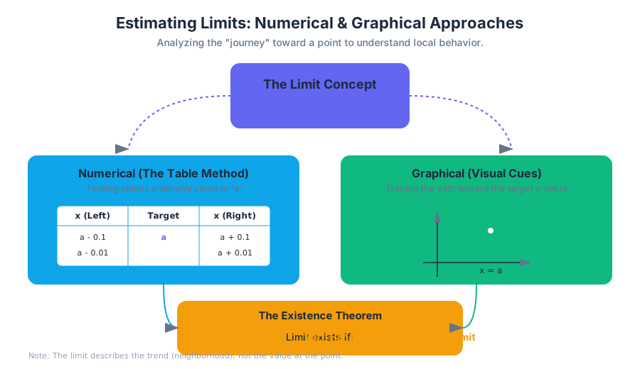
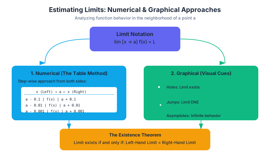
2. Numerical Estimation: The Table Method
Numerical estimation involves constructing a table of values where $x$ increments toward the target $a$ from both the left ($x < a$) and the right ($x > a$). This is often the first tool used when a function is too complex for immediate algebraic simplification.
How It Works: The "Delta-Stepping" Algorithm
- Identify the target $a$.
- Select a sequence of $x$-values approaching $a$ from the left (e.g., $a-0.1, a-0.01, a-0.001$).
- Select a sequence of $x$-values approaching $a$ from the right (e.g., $a+0.1, a+0.01, a+0.001$).
- Evaluate $f(x)$ for each value.
- Observe the trend. If $f(x)$ approaches the same value $L$ from both sides, we estimate the limit as $L$.
Numerical Example: $\lim_{x \to 0} \frac{\sin(x)}{x}$
This is a classic "indeterminate" form ($0/0$). Evaluating at $x=0$ is impossible, but the table reveals the truth:
| $x$ (Left) | $f(x)$ | $x$ (Right) | $f(x)$ |
|---|---|---|---|
| -0.1 | 0.99833 | 0.1 | 0.99833 |
| -0.01 | 0.99998 | 0.01 | 0.99998 |
| -0.001 | 0.99999 | 0.001 | 0.99999 |
Conclusion: As $x \to 0$, $f(x) \to 1$. Thus, $\lim_{x \to 0} \frac{\sin(x)}{x} = 1$.
import numpy as np

def estimate_limit(func, target, precision=5):
    """
    Numerically estimates the limit of a function as x approaches target.
    Uses a sequence of points getting progressively closer to the target.
    """
    # Generate points approaching from both sides
    deltas = [10**(-i) for i in range(1, precision + 2)]
    left_side = [target - d for d in deltas]
    right_side = [target + d for d in deltas]

    print(f"{'x (Approach)':<15} | {'f(x) Value':<15}")
    print("-" * 35)

    # Evaluate and print results
    for x in left_side + right_side:
        try:
            val = func(x)
            print(f"{x:<15.6f} | {val:<15.6f}")
        except ZeroDivisionError:
            print(f"{x:<15.6f} | UNDEFINED")

# Example: f(x) = (x^2 - 1) / (x - 1) as x -> 1
f = lambda x: (x**2 - 1) / (x - 1)
estimate_limit(f, 1)
3. Graphical Estimation: Tracing the Path
Graphical estimation is the process of visually inspecting the graph of $f(x)$ to determine the $y$-value the function approaches. This is particularly useful for identifying discontinuities and asymptotic behavior.
Visual Cues for Limits
- Holes (Removable Discontinuities): If the graph has a hole at $(a, L)$, the limit as $x \to a$ is $L$, even though $f(a)$ is undefined.
- Jumps (Jump Discontinuities): If the graph "breaks" and restarts at a different $y$-value, the two-sided limit does not exist.
- Vertical Asymptotes: If the graph shoots up to $+\infty$ or down to $-\infty$, the limit is unbounded.
Common Pitfalls in Graphical Analysis
A common mistake is confusing the dot with the path. If a graph has a hole at $(2, 4)$ but a solid dot at $(2, 6)$, the limit as $x \to 2$ is 4, not 6. The limit cares about where the path is leading, not where the point actually is.
4. One-Sided Limits
A two-sided limit exists if and only if the behavior from the left matches the behavior from the right. In many cases, specifically with piecewise functions, we must evaluate these independently.
Theorem: Existence of a Limit $\lim_{x \to a} f(x) = L$ if and only if $\lim_{x \to a^-} f(x) = L$ AND $\lim_{x \to a^+} f(x) = L$.
Notation
- $\lim_{x \to a^-} f(x)$: The limit as $x$ approaches $a$ from the left (values slightly smaller than $a$).
- $\lim_{x \to a^+} f(x)$: The limit as $x$ approaches $a$ from the right (values slightly larger than $a$).
Failure to Exist (DNE)
There are three primary reasons a limit fails to exist:
- Jump Discontinuity: Left-hand limit $\neq$ right-hand limit.
- Unbounded Behavior: The function approaches $\pm \infty$.
- Oscillating Behavior: The function fluctuates infinitely fast as it nears $a$ (e.g., $f(x) = \sin(1/x)$ as $x \to 0$).
\begin{aligned}
&\text{Formal } \epsilon-\delta \text{ Definition of a Limit:} \\
&\forall \epsilon > 0, \exists \delta > 0 \text{ such that } \\
&0 < |x - a| < \delta \implies |f(x) - L| < \epsilon
\end{aligned}
5. Unbounded Limits and Vertical Asymptotes
When $f(x)$ increases or decreases without bound as $x \to a$, we say the limit is infinite. While $\infty$ is not a real number, we use this notation to describe the specific type of non-existence.
Categorizing Unbounded Behavior
| Behavior | Notation | Graphical Feature |
|---|---|---|
| Increases without bound | $\lim_{x \to a} f(x) = \infty$ | Both sides shoot upward. |
| Decreases without bound | $\lim_{x \to a} f(x) = -\infty$ | Both sides shoot downward. |
| Mixed infinite behavior | $\text{Limit DNE}$ | One side goes to $+\infty$, other to $-\infty$. |
Vertical Asymptotes
If $\lim_{x \to a^+} f(x) = \pm \infty$ or $\lim_{x \to a^-} f(x) = \pm \infty$, then the line $x = a$ is a vertical asymptote of the graph of $f$.
6. Implementation and Tools
In professional practice, we rarely build tables by hand. We use computational engines to verify limits, especially when dealing with complex transcendental functions.
Using CLI Tools for Quick Estimation
For a quick check of a function's behavior near a point, developers often use bc (arbitrary precision calculator) or simple one-liners in shells that support math.
# Using Python CLI to check behavior of (1+x)^(1/x) as x -> 0 (Definition of e)
# We test 0.001, 0.0001, 0.00001
python3 -c "f = lambda x: (1+x)**(1/x); [print(f'x: {x}, f(x): {f(x)}') for x in [0.001, 0.0001, 0.00001]]"

# Output:
# x: 0.001, f(x): 2.7169239322355936
# x: 0.0001, f(x): 2.7181459268249255
# x: 1e-05, f(x): 2.7182682371922975
# (Approaching e ≈ 2.71828)
7. Summary of Limit Behaviors
To master limits, one must be able to synthesize the numerical data with the graphical representation.
| Scenario | Numerical Observation | Graphical Observation | Limit Status |
|---|---|---|---|
| Continuous Point | Values converge to $f(a)$ from both sides. | Smooth line passing through $(a, f(a))$. | Exists (equals $f(a)$). |
| Removable Hole | Values converge to $L$ from both sides. | A hole at $(a, L)$. | Exists (equals $L$). |
| Jump | Left side $\to L_1$, Right side $\to L_2$. | Path "breaks" and jumps vertically. | DNE. |
| Vertical Asymptote | Values grow extremely large/small. | Graph follows a vertical line to $\pm \infty$. | DNE (or $\pm \infty$). |
| Oscillation | Values bounce between extremes (e.g., -1 and 1). | Graph becomes a solid "blur" of color near $a$. | DNE. |
Pitfall: The "Precision Trap"
When estimating numerically, be wary of calculator rounding. If you approach a limit too closely (e.g., $10^{-15}$), floating-point errors in computer hardware can make a function appear to approach zero or infinity when it actually doesn't. Always look at the trend across several orders of magnitude ($10^{-1}, 10^{-2}, 10^{-3}$) rather than relying on a single, extremely small delta.
Final Insights
Estimating limits numerically and graphically is not just a "prelude" to algebra; it is a vital diagnostic skill. In the real world, functions are often defined by data points rather than clean equations. In these cases, the numerical approach is the only approach. By mastering the ability to read trends in tables and paths in graphs, you develop the mathematical "vision" required to understand the local behavior of any system, no matter how complex.
Differentiation: Definition and Fundamental Rules
Key concepts: Derivative as a Limit · Instantaneous Rate of Change · Power Rule · Product and Quotient Rules · Trigonometric and Exponential Derivatives
Defining the derivative as a rate of change and mastering basic rules for calculation.
Differentiation: Definition and Fundamental Rules
Differentiation is the mathematical process of determining the derivative of a function, a concept that serves as the cornerstone of modern calculus. While algebra allows us to calculate the average rate of change over a discrete interval, differentiation provides the tools to calculate the instantaneous rate of change at a single, infinitesimal point. This transition from the static to the dynamic is what enabled the scientific revolution, providing the language necessary to describe motion, electromagnetism, and the optimization of complex systems.
The Derivative as a Limit
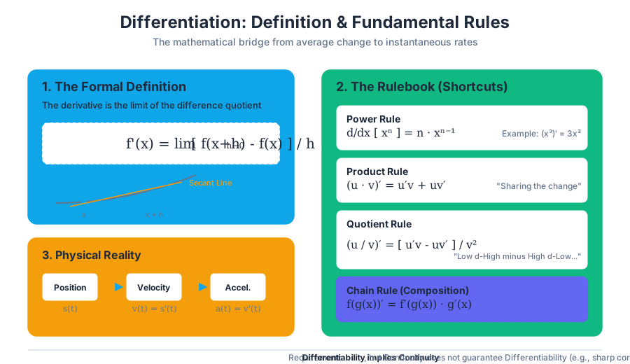
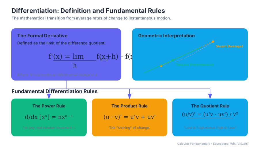
At its most fundamental level, the derivative is defined as the limit of the difference quotient. To understand this, imagine a curve defined by $f(x)$. If we pick two points on this curve, $(x, f(x))$ and $(x+h, f(x+h))$, the slope of the secant line connecting them is given by the ratio of the change in $y$ to the change in $x$.
Definition: The Formal Derivative The derivative of a function $f(x)$ with respect to $x$, denoted as $f'(x)$ or $\frac{dy}{dx}$, is defined as: $$f'(x) = \lim_{h \to 0} \frac{f(x+h) - f(x)}{h}$$ provided the limit exists.
Why the Limit Matters
The "problem" of the tangent line is that a single point does not have a slope; slope requires two points ($\frac{\Delta y}{\Delta x}$). By introducing the variable $h$ (the distance between two points) and shrinking it toward zero, we observe the behavior of the secant line as it converges into the tangent line. This limit allows us to capture the "slope" of the curve at a point where $\Delta x$ is effectively zero, yet the ratio remains finite and defined.
Numerical Implementation
In computational science, we often approximate this limit using a very small $h$. This is known as the Finite Difference Method.
def numerical_derivative(f, x, h=1e-7):
    """
    Computes the numerical approximation of the derivative
    using the symmetric difference quotient for higher accuracy.

    Args:
        f: The function to differentiate.
        x: The point at which to evaluate the derivative.
        h: The infinitesimal step size.
    """
    return (f(x + h) - f(x - h)) / (2 * h)

# Example: f(x) = x^2, f'(x) should be 2x. At x=5, f'(5)=10.
f = lambda x: x**2
print(f"Approximated derivative at x=5: {numerical_derivative(f, 5)}")
Instantaneous Rate of Change
The derivative is not merely a geometric construct; it is a physical reality. In physics, if $s(t)$ represents the position of an object over time $t$, the derivative $s'(t)$ represents its instantaneous velocity. The second derivative $s''(t)$ represents acceleration.
Comparison of Rates
| Feature | Average Rate of Change | Instantaneous Rate of Change |
|---|---|---|
| Geometry | Slope of the Secant Line | Slope of the Tangent Line |
| Interval | Over a finite interval $[a, b]$ | At a specific point $x = a$ |
| Formula | $\frac{f(b) - f(a)}{b - a}$ | $\lim_{h \to 0} \frac{f(a+h) - f(a)}{h}$ |
| Example | Average speed of a car over an hour | Speedometer reading at a specific second |
Differentiability and Continuity
A common misconception is that all continuous functions are differentiable. While differentiability implies continuity, the reverse is not true. For a derivative to exist at a point $x=c$, the limit from the left must equal the limit from the right: $$\lim_{h \to 0^-} \frac{f(c+h) - f(c)}{h} = \lim_{h \to 0^+} \frac{f(c+h) - f(c)}{h}$$
Failure of Differentiability
There are three primary cases where a function is continuous but not differentiable:
- Corners/Cusps: Where the slope changes abruptly (e.g., $f(x) = |x|$ at $x=0$).
- Vertical Tangents: Where the slope approaches infinity (e.g., $f(x) = \sqrt[3]{x}$ at $x=0$).
- Discontinuities: Any point where the function is not continuous (holes, jumps, or asymptotes).
The Power Rule
Calculating derivatives using the limit definition is algebraically taxing. The Power Rule is the first major shortcut discovered through the binomial expansion of the difference quotient.
The Power Rule For any real number $n$: $$\frac{d}{dx}[x^n] = nx^{n-1}$$
Derivation Sketch
For $f(x) = x^n$, the difference quotient involves $(x+h)^n$. Expanding this using the Binomial Theorem: $$(x+h)^n = x^n + nx^{n-1}h + \frac{n(n-1)}{2}x^{n-2}h^2 + \dots$$ When we subtract $f(x) = x^n$ and divide by $h$, all terms except the first ($nx^{n-1}$) still contain at least one factor of $h$. As $h \to 0$, those terms vanish, leaving only $nx^{n-1}$.
Power Rule Applications
| Function $f(x)$ | Rewritten Form | Derivative $f'(x)$ |
|---|---|---|
| $x^5$ | $x^5$ | $5x^4$ |
| $1/x^2$ | $x^{-2}$ | $-2x^{-3}$ or $-2/x^3$ |
| $\sqrt{x}$ | $x^{1/2}$ | $\frac{1}{2}x^{-1/2}$ or $\frac{1}{2\sqrt{x}}$ |
| $7$ | $7x^0$ | $0$ |
\begin{aligned}
&\text{Example: Differentiate } f(x) = 4x^3 - \frac{2}{x} + 5 \\
&f(x) = 4x^3 - 2x^{-1} + 5 \\
&f'(x) = \frac{d}{dx}[4x^3] - \frac{d}{dx}[2x^{-1}] + \frac{d}{dx}[5] \\
&f'(x) = (4 \cdot 3)x^{3-1} - (2 \cdot -1)x^{-1-1} + 0 \\
&f'(x) = 12x^2 + 2x^{-2} = 12x^2 + \frac{2}{x^2}
\end{aligned}
The Product and Quotient Rules
When functions are multiplied or divided, the derivative is not simply the product or quotient of their individual derivatives. This is a frequent source of error for beginners.
The Product Rule
If $u$ and $v$ are differentiable functions of $x$: $$\frac{d}{dx}[u \cdot v] = u'v + uv'$$ Insight: Think of this as the "sharing" of change. The total change is the rate of change of the first times the second, plus the first times the rate of change of the second.
The Quotient Rule
If $u$ and $v$ are differentiable functions of $x$: $$\frac{d}{dx}\left[\frac{u}{v}\right] = \frac{u'v - uv'}{v^2}$$ Mnemonic: "Low d-High minus High d-Low, over the square of what's below."
Comparison of Rules
| Rule | Formula | When to Use |
|---|---|---|
| Product | $(uv)' = u'v + uv'$ | When $f(x)$ is a product of two variable expressions. |
| Quotient | $(u/v)' = \frac{u'v - uv'}{v^2}$ | When $f(x)$ is a fraction with variables in the denominator. |
Transcendental Functions
Transcendental functions—those that "transcend" algebra—have unique derivative properties. The most notable is the natural exponential function $e^x$.
Exponential and Logarithmic Derivatives
The function $f(x) = e^x$ is the only non-zero function that is its own derivative. This makes it the fundamental solution to growth-rate problems.
- $\frac{d}{dx}[e^x] = e^x$
- $\frac{d}{dx}[\ln(x)] = \frac{1}{x}$
- $\frac{d}{dx}[a^x] = a^x \ln(a)$
Trigonometric Derivatives
Trigonometric derivatives are periodic and cyclic. The derivative of sine is cosine, while the derivative of cosine is negative sine.
| Function | Derivative |
|---|---|
| $\sin(x)$ | $\cos(x)$ |
| $\cos(x)$ | $-\sin(x)$ |
| $\tan(x)$ | $\sec^2(x)$ |
| $\cot(x)$ | $-\csc^2(x)$ |
| $\sec(x)$ | $\sec(x)\tan(x)$ |
| $\csc(x)$ | $-\csc(x)\cot(x)$ |
High-Level Implementation: Automatic Differentiation
In modern machine learning (like PyTorch or TensorFlow), derivatives are not calculated via the Power Rule or limits, but via Dual Numbers or Computational Graphs. Below is a conceptual look at how a "Dual Number" system tracks derivatives automatically.
#include <iostream>

// A simple Dual Number class for Automatic Differentiation
struct Dual {
    double val; // The value of the function
    double der; // The value of the derivative

    Dual(double v, double d = 0.0) : val(v), der(d) {}

    // Overload + for (u + v)' = u' + v'
    Dual operator+(const Dual& other) const {
        return Dual(val + other.val, der + other.der);
    }

    // Overload * for Product Rule: (uv)' = u'v + uv'
    Dual operator*(const Dual& other) const {
        return Dual(val * other.val, der * other.val + val * other.der);
    }
};

int main() {
    // Evaluate f(x) = x^2 at x = 5
    // x is the variable, so its derivative dx/dx is 1.0
    Dual x(5.0, 1.0);
    Dual f = x * x;

    std::cout << "f(5) = " << f.val << std::endl;      // Output: 25
    std::cout << "f'(5) = " << f.der << std::endl;     // Output: 10
    return 0;
}
Worked Example: Combining the Rules
Let us find the derivative of the complex function: $$y = \frac{x^2 e^x}{\sin(x)}$$
Step 1: Identify the structure. This is a quotient where the numerator is a product. Let $u = x^2 e^x$ and $v = \sin(x)$.
Step 2: Differentiate the numerator ($u$) using the Product Rule. $u = (x^2)(e^x)$ $u' = (2x)(e^x) + (x^2)(e^x) = e^x(2x + x^2)$
Step 3: Differentiate the denominator ($v$). $v = \sin(x)$ $v' = \cos(x)$
Step 4: Apply the Quotient Rule. $$y' = \frac{u'v - uv'}{v^2}$$ $$y' = \frac{[e^x(2x + x^2)]\sin(x) - [x^2 e^x]\cos(x)}{(\sin(x))^2}$$
Step 5: Simplify. $$y' = \frac{x e^x [(2+x)\sin(x) - x\cos(x)]}{\sin^2(x)}$$
Common Pitfalls and Edge Cases
- The Constant Rule Confusion: Beginners often try to apply the Power Rule to constants. Remember: $\frac{d}{dx}[5] = 0$, not $5x^{-1}$. A constant has no rate of change.
- The "Linearity" Trap: Thinking $\frac{d}{dx}[f(x)g(x)] = f'(x)g'(x)$. This is the most common error in calculus. Always use the Product Rule.
- Negative Exponents: When differentiating $x^{-3}$, the result is $-3x^{-4}$. Note that $-4$ is less than $-3$. Students often incorrectly write $-3x^{-2}$.
- The $e^x$ vs. $x^e$ Distinction:
- $\frac{d}{dx}[e^x] = e^x$ (Exponential Rule)
- $\frac{d}{dx}[x^e] = ex^{e-1}$ (Power Rule)
- Chain Rule Neglect: While not the focus of this section, many functions require the Chain Rule (e.g., $\sin(2x)$). Differentiating $\sin(2x)$ as $\cos(2x)$ is a common mistake; the correct answer is $2\cos(2x)$.
Summary of Rules for Quick Reference
| Rule Name | Mathematical Notation |
|---|---|
| Constant | $\frac{d}{dx}[c] = 0$ |
| Constant Multiple | $\frac{d}{dx}[cf(x)] = cf'(x)$ |
| Sum/Difference | $\frac{d}{dx}[f \pm g] = f' \pm g'$ |
| Power Rule | $\frac{d}{dx}[x^n] = nx^{n-1}$ |
| Product Rule | $\frac{d}{dx}[uv] = u'v + uv'$ |
| Quotient Rule | $\frac{d}{dx}[u/v] = \frac{u'v - uv'}{v^2}$ |
| Exponential | $\frac{d}{dx}[e^x] = e^x$ |
| Natural Log | $\frac{d}{dx}[\ln x] = 1/x$ |
| Sine | $\frac{d}{dx}[\sin x] = \cos x$ |
| Cosine | $\frac{d}{dx}[\cos x] = -\sin x$ |
Advanced Differentiation: Chain Rule and Implicit Differentiation
Key concepts: Chain Rule · Composite Functions · Implicit Differentiation · Inverse Function Derivatives · Higher-Order Derivatives
Techniques for differentiating complex composite functions and non-explicit equations.
Advanced Differentiation: Chain Rule and Implicit Differentiation
In the foundational study of calculus, we often treat functions as isolated entities—simple mappings where an input $x$ directly produces an output $y$. However, the real world rarely operates in such isolation. Systems are nested, variables are intertwined, and dependencies are often hidden within complex equations.
To navigate these complexities, we must move beyond basic power and product rules into Advanced Differentiation. This domain focuses on the Chain Rule (the calculus of nested systems), Implicit Differentiation (the calculus of intertwined variables), and the derivatives of Inverse Functions. Mastering these techniques is not merely an academic exercise; it is the prerequisite for understanding backpropagation in neural networks, orbital mechanics in aerospace engineering, and the sensitivity analysis of financial derivatives.
The Chain Rule: Differentiating Composite Functions
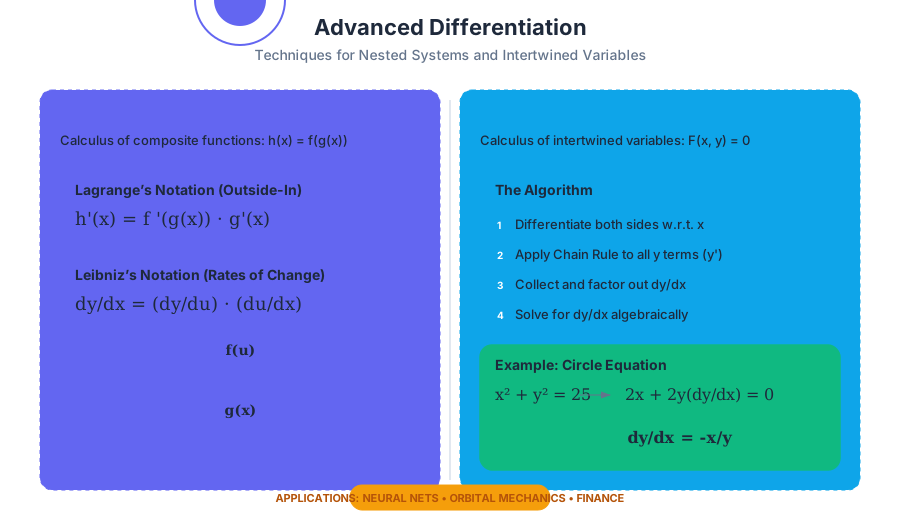
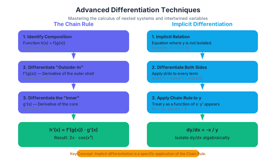
The Chain Rule is arguably the most important tool in a mathematician’s arsenal. It allows us to compute the derivative of a composite function—a function inside another function. If we define $h(x) = f(g(x))$, the Chain Rule provides the mechanism to find $h'(x)$ by decomposing the rate of change into its constituent parts.
1. Formal Definition and Notation
There are two primary ways to express the Chain Rule, each offering a different conceptual lens:
-
Lagrange’s Notation: If $h(x) = f(g(x))$, then: $$h'(x) = f'(g(x)) \cdot g'(x)$$ This emphasizes the "outside-in" approach: differentiate the outer function while keeping the inner function intact, then multiply by the derivative of the inner function.
-
Leibniz’s Notation: If $y = f(u)$ and $u = g(x)$, then: $$\frac{dy}{dx} = \frac{dy}{du} \cdot \frac{du}{dx}$$ This emphasizes the "rate of change" perspective: the total change is the product of the intermediate rates of change, much like a series of gears where the final speed depends on the ratio of every gear in the sequence.
2. The Mechanics of "Outside-In"
When applying the Chain Rule, we treat the inner function $g(x)$ as a single variable (often called $u$). We differentiate the "shell" first.
Theorem: The Chain Rule Let $g$ be differentiable at $x$ and let $f$ be differentiable at $g(x)$. Then the composite function $h = f \circ g$ is differentiable at $x$ and $h'(x) = f'(g(x))g'(x)$.
3. Common Chain Rule Patterns
| Function Type | General Form $y = f(g(x))$ | Derivative $y'$ |
|---|---|---|
| Power of a Function | $[g(x)]^n$ | $n[g(x)]^{n-1} \cdot g'(x)$ |
| Exponential | $e^{g(x)}$ | $e^{g(x)} \cdot g'(x)$ |
| Trigonometric | $\sin(g(x))$ | $\cos(g(x)) \cdot g'(x)$ |
| Logarithmic | $\ln(g(x))$ | $\frac{1}{g(x)} \cdot g'(x)$ |
4. Implementation Example: Automatic Differentiation
In modern computational science, the Chain Rule is implemented via Automatic Differentiation (AD). Below is a Python conceptualization of how a "Forward Mode" AD system tracks derivatives using the Chain Rule.
import numpy as np

class DualNumber:
    """
    A dual number (a + bε) used for forward-mode automatic differentiation.
    'val' represents the function value f(x).
    'der' represents the derivative value f'(x).
    """
    def __init__(self, val, der=1.0):
        self.val = val
        self.der = der

    def __add__(self, other):
        return DualNumber(self.val + other.val, self.der + other.der)

    def __mul__(self, other):
        # Product Rule: (uv)' = u'v + uv'
        return DualNumber(self.val * other.val,
                          self.der * other.val + self.val * other.der)

    def sin(self):
        # Chain Rule: d/dx sin(u) = cos(u) * u'
        return DualNumber(np.sin(self.val), np.cos(self.val) * self.der)

    def exp(self):
        # Chain Rule: d/dx e^u = e^u * u'
        return DualNumber(np.exp(self.val), np.exp(self.val) * self.der)

# Example: f(x) = exp(sin(x)) at x = 0
x = DualNumber(0.0, 1.0)
f_x = x.sin().exp()

print(f"Value: {f_x.val}")      # exp(sin(0)) = 1.0
print(f"Derivative: {f_x.der}") # exp(sin(0)) * cos(0) = 1.0
Implicit Differentiation: Solving Intertwined Relations
Most functions we encounter in early calculus are explicit: $y$ is isolated on one side ($y = x^2 + 5$). However, many mathematical models are implicit, meaning $y$ is buried within the equation (e.g., $x^2 + y^2 = 25$).
1. What is Implicit Differentiation?
Implicit differentiation is the process of differentiating both sides of an equation with respect to $x$, treating $y$ as a differentiable function of $x$. This is essentially a specialized application of the Chain Rule. Whenever we differentiate a term containing $y$, we must append a $\frac{dy}{dx}$ (or $y'$) factor.
2. The Algorithm
- Differentiate both sides of the equation with respect to $x$.
- Apply the Chain Rule to all terms involving $y$ (the derivative of $y^n$ is $ny^{n-1} \cdot \frac{dy}{dx}$).
- Collect all terms containing $\frac{dy}{dx}$ on one side of the equation.
- Factor out $\frac{dy}{dx}$.
- Solve for $\frac{dy}{dx}$ by dividing.
3. Worked Example: The Folium of Descartes
Consider the equation $x^3 + y^3 = 6xy$. To find the slope of the tangent line at any point $(x, y)$:
\begin{aligned}
\frac{d}{dx}[x^3 + y^3] &= \frac{d}{dx}[6xy] \\
3x^2 + 3y^2 \frac{dy}{dx} &= 6(y + x \frac{dy}{dx}) \quad \text{(using Product Rule on 6xy)} \\
3x^2 + 3y^2 y' &= 6y + 6xy' \\
3y^2 y' - 6xy' &= 6y - 3x^2 \\
y'(3y^2 - 6x) &= 6y - 3x^2 \\
y' &= \frac{6y - 3x^2}{3y^2 - 6x} = \frac{2y - x^2}{y^2 - 2x}
\end{aligned}
4. Why It Matters: Orthogonal Trajectories
Implicit differentiation allows us to find families of curves that intersect others at right angles (orthogonal trajectories). This is vital in physics for mapping electric field lines relative to equipotential surfaces.
Derivatives of Inverse Functions
If a function $f$ has an inverse $f^{-1}$, there is a direct relationship between their derivatives. This is highly useful when the derivative of the original function is easy to compute, but the inverse is difficult to differentiate directly.
1. The Inverse Function Theorem
If $f$ is a differentiable function that is one-to-one on an interval $I$, and $f'(f^{-1}(a)) \neq 0$, then the inverse function $g = f^{-1}$ is differentiable at $a$ and: $$g'(a) = \frac{1}{f'(g(a))}$$
In simpler terms, the slope of the inverse function at point $(a, b)$ is the reciprocal of the slope of the original function at point $(b, a)$.
2. Inverse Trigonometric Functions
We derive the derivatives of inverse trig functions using implicit differentiation. For example, to find the derivative of $y = \arcsin(x)$:
- Rewrite as $\sin(y) = x$.
- Differentiate implicitly: $\cos(y) \cdot \frac{dy}{dx} = 1$.
- Solve for $\frac{dy}{dx} = \frac{1}{\cos(y)}$.
- Use the identity $\cos(y) = \sqrt{1 - \sin^2(y)}$. Since $\sin(y) = x$, then $\cos(y) = \sqrt{1 - x^2}$.
- Result: $\frac{d}{dx}[\arcsin(x)] = \frac{1}{\sqrt{1 - x^2}}$.
3. Summary of Inverse Trig Derivatives
| Function $f(x)$ | Derivative $f'(x)$ | Domain Restrictions |
|---|---|---|
| $\arcsin(x)$ | $\frac{1}{\sqrt{1-x^2}}$ | $-1 < x < 1$ |
| $\arccos(x)$ | $-\frac{1}{\sqrt{1-x^2}}$ | $-1 < x < 1$ |
| $\arctan(x)$ | $\frac{1}{1+x^2}$ | All real $x$ |
| $\text{arcsec}(x)$ | $\frac{1}{\vert x\vert \sqrt{x^2-1}}$ | $\vert x\vert > 1$ |
Higher-Order Derivatives
A derivative is itself a function, and if it is differentiable, we can differentiate it again. This process yields higher-order derivatives.
1. Notation and Interpretation
- First Derivative ($f'$ or $\frac{dy}{dx}$): Velocity; the rate of change of position.
- Second Derivative ($f''$ or $\frac{d^2y}{dx^2}$): Acceleration; the rate of change of velocity.
- Third Derivative ($f'''$ or $\frac{d^3y}{dx^3}$): Jerk; the rate of change of acceleration.
2. Concavity and the Second Derivative
The second derivative tells us about the "bending" of the graph:
- If $f''(x) > 0$, the graph is concave up (holds water).
- If $f''(x) < 0$, the graph is concave down (sheds water).
- An inflection point occurs where $f''(x)$ changes sign.
3. Real-World Usage: Physics Simulation
In systems programming, higher-order derivatives are used to solve differential equations for motion. Below is a Rust example of a simple Euler integrator that uses acceleration (2nd derivative) to update state.
struct Particle {
    position: f64,
    velocity: f64,
    mass: f64,
}

impl Particle {
    // Applying a force calculates acceleration (2nd derivative of position)
    // a = F / m
    fn update(&mut self, force: f64, dt: f64) {
        let acceleration = force / self.mass;

        // Update velocity (integral of acceleration)
        self.velocity += acceleration * dt;

        // Update position (integral of velocity)
        self.position += self.velocity * dt;
    }
}

fn main() {
    let mut p = Particle { position: 0.0, velocity: 0.0, mass: 1.0 };
    let constant_force = 9.8; // Gravity
    let delta_time = 0.1;

    for step in 0..10 {
        p.update(constant_force, delta_time);
        println!("Step {}: Position = {:.2}, Velocity = {:.2}",
                 step, p.position, p.velocity);
    }
}
Pitfalls and Best Practices
Even experienced practitioners stumble on advanced differentiation. Here are the most common points of failure:
1. The "Missing Link" in the Chain Rule
The most common error is forgetting to multiply by the derivative of the inner function.
- Wrong: $\frac{d}{dx}(\sin(x^2)) = \cos(x^2)$
- Right: $\frac{d}{dx}(\sin(x^2)) = \cos(x^2) \cdot 2x$
2. Misinterpreting Inverse Notation
The notation $f^{-1}(x)$ refers to the inverse function, not the reciprocal $1/f(x)$.
- $(\sin(x))^{-1} = \csc(x)$
- $\sin^{-1}(x) = \arcsin(x)$ These have entirely different derivatives.
3. Implicit Differentiation of Constants
When differentiating an equation like $x^2 + y^2 = 25$, students often forget to differentiate the constant on the right side.
- Wrong: $2x + 2yy' = 25$
- Right: $2x + 2yy' = 0$
4. Higher-Order Leibniz Notation
The notation $\frac{d^2y}{dx^2}$ is often confusing. The "2" is placed differently in the numerator and denominator because it represents the operator $(\frac{d}{dx})$ being applied twice to $y$: $$\frac{d}{dx} \left( \frac{dy}{dx} \right) = \frac{d^2y}{dx^2}$$
Comparison of Differentiation Methods
| Method | Best Used For | Key Difficulty |
|---|---|---|
| Power/Product/Quotient | Explicit polynomial/rational functions | Managing algebraic expansion |
| Chain Rule | Nested functions, $f(g(x))$ | Identifying the "inner" vs "outer" layers |
| Implicit | Circles, ellipses, non-functions | Isolating $y'$ algebraically |
| Logarithmic | Variable-to-variable powers ($x^x$) | Remembering to multiply by $y$ at the end |
Contextual Applications of Differentiation
Key concepts: Straight-line Motion · Related Rates · Local Linearity · L'Hôpital's Rule · Position, Velocity, and Acceleration
Applying derivatives to solve real-world problems involving motion, rates, and approximations.
Contextual Applications of Differentiation
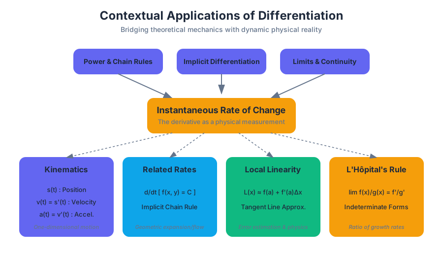
The transition from the theoretical mechanics of differentiation—the Power Rule, Chain Rule, and Implicit Differentiation—to their Contextual Applications represents the shift from pure mathematics to engineering, physics, and economics. In this domain, the derivative is no longer just a limit of a difference quotient; it is an instantaneous rate of change that governs the motion of satellites, the expansion of viral outbreaks, and the optimization of industrial processes.
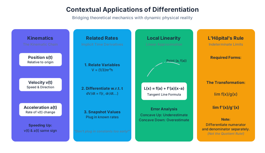
This article explores the four pillars of applied differentiation: Straight-line Motion, Related Rates, Local Linearity, and L'Hôpital's Rule. Each concept serves as a bridge between a static mathematical model and a dynamic physical reality.
Straight-line Motion: Kinematics in One Dimension
Straight-line motion, or rectilinear motion, is the study of an object moving along a fixed path (typically the x-axis or y-axis). In this context, we define three fundamental functions of time $t$: Position, Velocity, and Acceleration.
The Kinematic Hierarchy
The relationship between these quantities is hierarchical, defined by successive differentiation with respect to time.
Definition: The Kinematic Chain
- Position $s(t)$: The location of the particle relative to the origin at time $t$.
- Velocity $v(t) = s'(t)$: The instantaneous rate of change of position. It indicates both speed and direction.
- Acceleration $a(t) = v'(t) = s''(t)$: The instantaneous rate of change of velocity.
| Quantity | Notation | Relationship | Physical Interpretation |
|---|---|---|---|
| Position | $s(t)$ | $s(t)$ | Where the object is. |
| Velocity | $v(t)$ | $\frac{ds}{dt}$ | How fast and in what direction it is moving. |
| Acceleration | $a(t)$ | $\frac{dv}{dt} = \frac{d^2s}{dt^2}$ | How the velocity is changing. |
| Speed | $ | v(t) | $ |
| Displacement | $\Delta s$ | $s(t_2) - s(t_1)$ | Net change in position. |
Analyzing Particle Behavior
To fully describe motion, we must interpret the signs and zeros of these derivatives:
- Direction of Motion: If $v(t) > 0$, the particle moves in the positive direction (right/up). If $v(t) < 0$, it moves in the negative direction (left/down).
- Turning Points: A particle changes direction only when $v(t) = 0$ and $v(t)$ changes sign.
- Speeding Up vs. Slowing Down:
- Speeding Up: $v(t)$ and $a(t)$ have the same sign (both positive or both negative).
- Slowing Down: $v(t)$ and $a(t)$ have opposite signs.
Worked Example: Numerical Simulation
Consider a particle whose position is defined by $s(t) = t^3 - 6t^2 + 9t$ for $t \ge 0$.
- $v(t) = 3t^2 - 12t + 9 = 3(t-1)(t-3)$.
- $a(t) = 6t - 12 = 6(t-2)$.
- The particle is at rest at $t=1$ and $t=3$.
- At $t=1.5$, $v(1.5)$ is negative and $a(1.5)$ is negative. Since signs match, the particle is speeding up in the negative direction.
import numpy as np

def analyze_motion(t_range, position_func):
    """
    Low-level numerical analysis of 1D motion.
    Uses central difference for high-precision derivative estimation.
    """
    dt = 1e-5
    t = np.array(t_range)

    # Position
    s = position_func(t)

    # Velocity (First Derivative)
    v = (position_func(t + dt) - position_func(t - dt)) / (2 * dt)

    # Acceleration (Second Derivative)
    a = (position_func(t + dt) - 2*position_func(t) + position_func(t - dt)) / (dt**2)

    # Speed
    speed = np.abs(v)

    # Logical state: Speeding up if v and a have same sign
    speeding_up = (v * a) > 0

    return {
        "time": t,
        "velocity": v,
        "acceleration": a,
        "is_speeding_up": speeding_up
    }

# Example: s(t) = t^3 - 6t^2 + 9t
results = analyze_motion([0.5, 1.5, 2.5], lambda t: t**3 - 6*t**2 + 9*t)
print(f"At t=1.5: Velocity={results['velocity'][1]:.2f}, Speeding Up={results['is_speeding_up'][1]}")
Related Rates: The Chain Rule in Context
Related Rates problems involve finding the rate at which one quantity changes by relating it to other quantities whose rates of change are known. This is a direct application of Implicit Differentiation with respect to time $t$.
The Procedural Framework
Solving these problems requires a disciplined approach to distinguish between "constants" (values that never change) and "instantaneous values" (values that are only true at a specific moment).
- Identify Variables: List all given rates (e.g., $dr/dt$) and the rate to be found (e.g., $dV/dt$).
- Relate the Variables: Write an equation that connects the variables (e.g., Geometry formulas like $V = \frac{4}{3}\pi r^3$).
- Differentiate: Use the Chain Rule to differentiate both sides with respect to $t$.
- Substitute and Solve: Plug in the "snapshot" values only after differentiation.
| Scenario | Primary Equation | Differentiated Equation (w.r.t $t$) |
|---|---|---|
| Expanding Circle | $A = \pi r^2$ | $\frac{dA}{dt} = 2\pi r \frac{dr}{dt}$ |
| Sliding Ladder | $x^2 + y^2 = L^2$ | $2x\frac{dx}{dt} + 2y\frac{dy}{dt} = 0$ |
| Conical Tank | $V = \frac{1}{3}\pi r^2 h$ | $\frac{dV}{dt} = \frac{1}{3}\pi (2rh \frac{dr}{dt} + r^2 \frac{dh}{dt})$ |
| Shadow Length | $\frac{x+s}{H} = \frac{s}{h}$ | (Use similar triangles to relate $dx/dt$ and $ds/dt$) |
The Cone Problem: A Classic Derivation
In many related rates problems, such as a leaking conical tank, we have too many variables ($r$ and $h$). We must use the geometry of the container to find a relationship between $r$ and $h$ (usually via similar triangles) to reduce the equation to a single variable before differentiating.
\text{Given: } V = \frac{1}{3}\pi r^2 h \text{ and } \frac{r}{h} = \frac{R_{max}}{H_{max}} = k \\
\text{Substitute } r = kh: \\
V = \frac{1}{3}\pi (kh)^2 h = \frac{\pi k^2}{3} h^3 \\
\text{Differentiate w.r.t } t: \\
\frac{dV}{dt} = \pi k^2 h^2 \frac{dh}{dt} \\
\text{Solve for } \frac{dh}{dt}: \\
\frac{dh}{dt} = \frac{dV/dt}{\pi k^2 h^2}
Common Pitfalls in Related Rates
- Premature Substitution: Plugging in a constant value for a variable before differentiating. If a value changes over time, it must remain a variable ($x, y, r$) until the derivative is taken.
- Sign Errors: If a distance is decreasing (e.g., water draining), the rate must be negative ($dV/dt < 0$).
- Units: Forgetting to reconcile units (e.g., mixing inches and feet).
Local Linearity and Linearization
Local Linearity is the principle that any differentiable function $f(x)$ looks like a straight line if you zoom in close enough to a point $(a, f(a))$. This line is the tangent line.
The Linearization Formula
The Linearization of $f$ at $a$, denoted $L(x)$, is simply the equation of the tangent line used as an approximation tool.
Theorem: Linearization For a function $f$ differentiable at $x=a$, the linear approximation is: $$L(x) = f(a) + f'(a)(x - a)$$ For $x$ values near $a$, $f(x) \approx L(x)$.
Differentials
While $L(x)$ approximates the function value, differentials approximate the change in the function value.
- Let $dx$ be an independent variable (the change in $x$).
- The differential $dy$ is defined as $dy = f'(x)dx$.
- $dy$ represents the change along the tangent line, whereas $\Delta y$ represents the actual change in the function.
| Term | Symbol | Definition |
|---|---|---|
| Actual Change | $\Delta y$ | $f(a + \Delta x) - f(a)$ |
| Approximate Change | $dy$ | $f'(a)dx$ |
| Error | $ | \Delta y - dy |
Real-World Application: Sensor Calibration
In embedded systems, calculating complex functions like $\sqrt{x}$ or $\ln(x)$ is computationally expensive. Engineers often use linearization to create "fast" approximations for sensors within a specific operating range.
/**
 * Linearization of f(x) = sqrt(x) at a = 64.
 * f(64) = 8, f'(x) = 1/(2*sqrt(x)), f'(64) = 1/16
 * L(x) = 8 + (1/16)(x - 64)
 */
float fast_sqrt_approx(float x) {
    // This approximation is highly accurate for x near 64 (e.g., 60 to 68)
    // Avoids expensive floating point sqrt() hardware calls
    const float f_a = 8.0f;
    const float f_prime_a = 0.0625f; // 1/16
    const float a = 64.0f;

    return f_a + f_prime_a * (x - a);
}

// Usage in a control loop
float sensor_val = 65.2;
float result = fast_sqrt_approx(sensor_val);
// Actual sqrt(65.2) ≈ 8.07465
// L(65.2) = 8 + 0.0625 * 1.2 = 8.075
Concavity and Error
The accuracy of a linear approximation depends on the concavity of the function:
- If $f''(x) > 0$ (Concave Up), the tangent line lies below the curve, so $L(x)$ is an underestimate.
- If $f''(x) < 0$ (Concave Down), the tangent line lies above the curve, so $L(x)$ is an overestimate.
L'Hôpital's Rule: Resolving Indeterminacy
When evaluating limits, we often encounter indeterminate forms like $0/0$ or $\infty/\infty$. These forms do not have a defined value; the limit depends on the "race" between the numerator and the denominator.
The Theorem
L'Hôpital's Rule Suppose $f$ and $g$ are differentiable and $g'(x) \neq 0$ near $a$ (except possibly at $a$). If: $$\lim_{x \to a} \frac{f(x)}{g(x)} = \frac{0}{0} \quad \text{or} \quad \lim_{x \to a} \frac{f(x)}{g(x)} = \frac{\pm \infty}{\pm \infty}$$ Then: $$\lim_{x \to a} \frac{f(x)}{g(x)} = \lim_{x \to a} \frac{f'(x)}{g'(x)}$$ provided the limit on the right exists.
Indeterminate Forms Summary
L'Hôpital's Rule applies directly only to quotients. Other indeterminate forms must be algebraically transformed into $0/0$ or $\infty/\infty$.
| Form | Type | Strategy |
|---|---|---|
| $0/0$ | Quotient | Apply L'Hôpital directly. |
| $\infty/\infty$ | Quotient | Apply L'Hôpital directly. |
| $0 \cdot \infty$ | Product | Rewrite as $\frac{f}{1/g}$ to get $0/0$ or $\infty/\infty$. |
| $\infty - \infty$ | Difference | Find a common denominator or factor out a term. |
| $1^\infty, 0^0, \infty^0$ | Power | Use natural logs: $y = f^g \implies \ln y = g \ln f$. |
Critical Warning: The Quotient Rule Trap
A common student error is to use the Quotient Rule when applying L'Hôpital's Rule.
- Correct: Differentiate the top and bottom separately: $\frac{f'(x)}{g'(x)}$.
- Incorrect: Differentiate the whole fraction: $\frac{f'g - fg'}{g^2}$.
Practical Example: Growth Rates
L'Hôpital's Rule is essential for comparing the growth of functions. For instance, to prove that exponential functions grow faster than any power function: $$\lim_{x \to \infty} \frac{e^x}{x^n}$$ Applying L'Hôpital's Rule $n$ times will eventually reduce the denominator to $n!$ (a constant) while the numerator remains $e^x$, showing the limit is $\infty$.
# Example of using a symbolic math tool (like SymPy via CLI) to verify limits
python3 -c "from sympy import limit, Symbol, exp; x = Symbol('x'); print(limit(exp(x)/x**2, x, 'oo'))"
# Output: oo
Synthesis: The Interconnectedness of Rates
The contextual applications of differentiation are not isolated topics; they are different perspectives on the same underlying truth: The derivative is the local linear behavior of a system.
- In Motion, we look at how position changes over time.
- In Related Rates, we look at how multiple geometric dimensions change over time.
- In Linearization, we use the rate of change to predict nearby values.
- In L'Hôpital's Rule, we compare the rates of change of two functions to determine their limiting ratio.
By mastering these applications, one gains the ability to decompose complex, dynamic systems into manageable, linear components—the hallmark of advanced scientific and engineering analysis.
- Position ($s(t)$): The location of an object at time $t$.
- Velocity ($v(t)$): $s'(t)$; the rate of change of position; includes direction.
- Acceleration ($a(t)$): $v'(t)$; the rate of change of velocity.
- Speeding Up: Occurs when velocity and acceleration have the same sign.
- Slowing Down: Occurs when velocity and acceleration have opposite signs.
- Related Rates: A method using implicit differentiation to find an unknown rate of change in terms of known rates.
- Linearization ($L(x)$): $f(a) + f'(a)(x-a)$; the tangent line approximation of a function near $x=a$.
- Differential ($dy$): $f'(x)dx$; the change in height along the tangent line.
- L'Hôpital's Rule: A limit evaluation method for $0/0$ or $\infty/\infty$ using $\lim f'(x)/g'(x)$.
- Indeterminate Form: A limit expression (like $0/0$) that requires further analysis to evaluate.
- True or False: If a particle's velocity is negative and its acceleration is positive, the particle is speeding up.
- Related Rates: A 10ft ladder leans against a wall. If the bottom slides away at 2ft/s, how fast is the top sliding down when the bottom is 6ft from the wall?
- Linearization: If $f(x) = \ln(x)$, what is the linearization $L(x)$ at $a=1$?
- L'Hôpital's: Evaluate $\lim_{x \to 0} \frac{\sin(5x)}{x}$.
- Concavity: If $f''(x) > 0$ on an interval, will the linear approximation $L(x)$ be an overestimate or an underestimate?
Answers: 1. False (Slowing down), 2. -1.5 ft/s, 3. $L(x) = x - 1$, 4. 5, 5. Underestimate.
Core Competencies for Contextual Differentiation:
- Kinematic Analysis:
- Be able to find when a particle is at rest ($v=0$).
- Determine intervals of motion (left/right).
- Calculate total distance traveled (sum of absolute displacements between turning points).
- Related Rates Mastery:
- Memorize volume/surface area for spheres, cones, and cylinders.
- Always differentiate with respect to $t$, not the variable itself (e.g., $\frac{d}{dt}[r^2] = 2r \frac{dr}{dt}$).
- Linearization & Differentials:
- Understand that $L(x)$ is just the tangent line.
- Recognize that $dy \approx \Delta y$ for small $dx$.
- L'Hôpital's Rule Proficiency:
- Always check for $0/0$ or $\infty/\infty$ before applying.
- Know how to convert $0 \cdot \infty$ and $1^\infty$ into quotient forms.
- Recognize when to stop (if the limit is no longer indeterminate).
Analytical Applications of Differentiation
Key concepts: Mean Value Theorem (MVT) · Extreme Value Theorem (EVT) · First and Second Derivative Tests · Concavity and Inflection Points · Optimization Problems
Using derivatives to analyze function behavior, including extrema, concavity, and optimization.
Analytical Applications of Differentiation
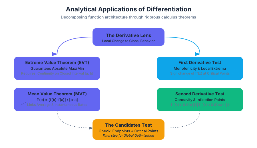
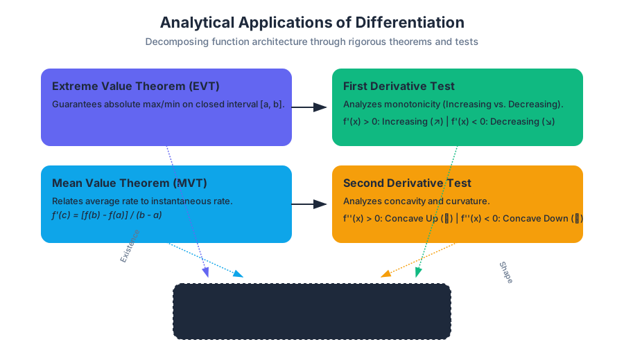
The study of differentiation extends far beyond the mere calculation of slopes. In the analytical realm, the derivative serves as a high-resolution lens through which we can decompose the behavior of functions, predict their long-term trajectories, and find optimal solutions to complex physical and economic problems. This section explores the rigorous theorems and tests that allow us to move from a local understanding of change to a global understanding of function architecture.
The Extreme Value Theorem (EVT)
The Extreme Value Theorem (EVT) is an existence theorem. It does not tell us where a maximum or minimum occurs, but it guarantees that under specific conditions, they must exist. This is the logical bedrock upon which all optimization is built.
The Extreme Value Theorem: If a function $f$ is continuous on a closed interval $[a, b]$, then $f$ must attain an absolute maximum and an absolute minimum at least once within that interval.
Why It Matters
In real-world engineering, we often operate within "constraints" (the closed interval). If you are designing a bridge, there is a maximum load it will face. If you are a chemist, there is a specific temperature range for a reaction. The EVT ensures that within these bounds, there is a "best" and "worst" case scenario to find.
The Candidates Test
To find these absolute extrema, we use the Candidates Test. We check the function values at:
- Critical Points: Where $f'(x) = 0$ or $f'(x)$ is undefined.
- Endpoints: The boundaries $a$ and $b$ of the interval.
| Feature | Absolute Extrema | Relative (Local) Extrema |
|---|---|---|
| Definition | The highest/lowest point on the entire domain/interval. | A point higher/lower than all nearby points. |
| Existence | Guaranteed on closed intervals by EVT. | Not guaranteed; depends on function shape. |
| Location | Can be at critical points OR endpoints. | Must be at critical points. |
| Requirement | $f(c) \geq f(x)$ for all $x$ in domain. | $f(c) \geq f(x)$ for $x$ in an open interval near $c$. |
The Mean Value Theorem (MVT)
If the EVT is about "where we are," the Mean Value Theorem (MVT) is about "how we got there." It bridges the gap between the average rate of change (algebra) and the instantaneous rate of change (calculus).
The Mean Value Theorem: If $f$ is continuous on $[a, b]$ and differentiable on $(a, b)$, then there exists at least one point $c$ in $(a, b)$ such that: $$f'(c) = \frac{f(b) - f(a)}{b - a}$$
The "Speed Trap" Analogy
Imagine you enter a toll road at 1:00 PM and exit 100 miles later at 2:00 PM. Your average speed was 100 mph. Even if a police officer didn't see you speeding, the MVT proves that at some specific moment $c$ between 1:00 and 2:00, your speedometer read exactly 100 mph.
Rolle's Theorem: A Special Case
Rolle's Theorem is a specific instance of the MVT where $f(a) = f(b)$. If you start and end at the same height, and the function is "smooth" (differentiable), there must be at least one point where the tangent line is horizontal ($f'(c) = 0$).
\begin{aligned}
&\text{Proof Sketch of MVT using Rolle's Theorem:} \\
&\text{1. Define a secant line equation: } g(x) = f(a) + \frac{f(b)-f(a)}{b-a}(x-a) \\
&\text{2. Create an auxiliary function: } h(x) = f(x) - g(x) \\
&\text{3. Note that } h(a) = 0 \text{ and } h(b) = 0. \\
&\text{4. By Rolle's Theorem, } \exists c \in (a, b) \text{ such that } h'(c) = 0. \\
&\text{5. } h'(x) = f'(x) - \frac{f(b)-f(a)}{b-a} \implies f'(c) = \frac{f(b)-f(a)}{b-a}.
\end{aligned}
Monotonicity and the First Derivative Test
To understand the "flow" of a function, we examine the sign of its first derivative. This allows us to categorize intervals of increase and decrease and identify local extrema.
Critical Points
A Critical Point occurs at $x = c$ if $f'(c) = 0$ or if $f'(c)$ does not exist. These are the only locations where a function can potentially change from increasing to decreasing.
The First Derivative Test
This test classifies critical points based on the behavior of $f'(x)$ as it "crosses" the point.
| Sign Change of $f'(x)$ | Conclusion at $x = c$ | Visual Interpretation |
|---|---|---|
| Positive to Negative | Local Maximum | A mountain peak ($\nearrow \bullet \searrow$) |
| Negative to Positive | Local Minimum | A valley floor ($\searrow \bullet \nearrow$) |
| No sign change | No Extremum | A "shelf" or point of inflection ($y=x^3$ at $x=0$) |
Implementation Example (Python)
In computational science, we often use symbolic math libraries to find these points precisely.
import sympy as sp

def analyze_extrema(expression_str, x_range):
    x = sp.symbols('x')
    f = sp.sympify(expression_str)

    # Calculate first derivative
    f_prime = sp.diff(f, x)

    # Find critical points within the domain
    critical_points = sp.solve(f_prime, x)

    results = []
    for cp in critical_points:
        # Check sign change using small epsilon
        left_val = f_prime.subs(x, cp - 0.01)
        right_val = f_prime.subs(x, cp + 0.01)

        if left_val > 0 and right_val < 0:
            classification = "Local Maximum"
        elif left_val < 0 and right_val > 0:
            classification = "Local Minimum"
        else:
            classification = "Saddle/Inflection"

        results.append((float(cp), classification))

    return results

# Example: f(x) = x^3 - 3x^2 + 2
print(analyze_extrema("x**3 - 3*x**2 + 2", (0, 5)))
Concavity and the Second Derivative Test
While the first derivative tells us the direction of a function, the second derivative $f''(x)$ tells us the Concavity—the way the function curves.
Concavity Definitions
- Concave Up ($f''(x) > 0$): The function is shaped like a cup ($\cup$). The slopes are increasing.
- Concave Down ($f''(x) < 0$): The function is shaped like a frown ($\cap$). The slopes are decreasing.
- Inflection Point: A point where the concavity changes (e.g., from up to down). This occurs where $f''(x) = 0$ or is undefined, and the sign of $f''(x)$ actually changes.
The Second Derivative Test
This is an alternative way to classify critical points. If $f'(c) = 0$:
- If $f''(c) > 0$, then $f$ has a local minimum at $c$.
- If $f''(c) < 0$, then $f$ has a local maximum at $c$.
- If $f''(c) = 0$, the test is inconclusive (use the First Derivative Test).
Global Optimization and Applied Modeling
Optimization is the process of finding the maximum or minimum value of a "target" function (the objective function) subject to certain constraints.
The Optimization Workflow
- Identify Variables: Determine what can be changed (e.g., $x$ for width, $y$ for height).
- Primary Equation: Write the formula for the quantity to be optimized (e.g., Area $A = xy$).
- Secondary Equation (Constraint): Use given info to relate variables (e.g., Perimeter $2x + 2y = 100$).
- Substitution: Reduce the primary equation to a single variable using the constraint.
- Differentiation: Find the derivative and set to zero to find critical points.
- Verification: Use the First or Second Derivative test to ensure it's the desired extremum.
Worked Example: The Maximum Volume Box
A sheet of cardboard 20in by 20in has squares of side $x$ cut out of the corners to form an open-top box. Find the value of $x$ that maximizes volume.
- Volume: $V(x) = (20 - 2x)(20 - 2x)x = 4x^3 - 80x^2 + 400x$
- Domain: $x \in [0, 10]$ (since $2x$ cannot exceed 20).
- Derivative: $V'(x) = 12x^2 - 160x + 400$
- Solve $V'(x) = 0$: $4(3x^2 - 40x + 100) = 0 \implies 4(3x - 10)(x - 10) = 0$.
- Critical Points: $x = 10/3$ and $x = 10$.
- Test: $V(10) = 0$ (minimum). $V(10/3) \approx 592.6$ in³.
- Result: The optimal cut is $3.33$ inches.
Performance-Critical Optimization (Rust)
In systems programming, we might implement numerical methods like Newton's Method to find these critical points when analytical solutions are impossible.
/// Finds the root of f'(x) = 0 using Newton's Method
/// f_prime: the first derivative
/// f_double_prime: the second derivative
fn find_critical_point(
    f_prime: fn(f64) -> f64,
    f_double_prime: fn(f64) -> f64,
    mut x_guess: f64
) -> f64 {
    let tolerance = 1e-10;
    let max_iterations = 1000;

    for _ in 0..max_iterations {
        let y = f_prime(x_guess);
        let y_prime = f_double_prime(x_guess);

        if y_prime.abs() < tolerance { break; }

        let next_x = x_guess - y / y_prime;
        if (next_x - x_guess).abs() < tolerance {
            return next_x;
        }
        x_guess = next_x;
    }
    x_guess
}

fn main() {
    // Example for f(x) = x^2 - 4x
    // f'(x) = 2x - 4, f''(x) = 2
    let cp = find_critical_point(|x| 2.0 * x - 4.0, |_| 2.0, 0.0);
    println!("Critical point found at: {}", cp);
}
Common Pitfalls and Edge Cases
Analytical differentiation is rigorous, but several "traps" exist for the unwary student or engineer.
- The $f''(c) = 0$ Trap: Many assume if the second derivative is zero, it's an inflection point. Consider $f(x) = x^4$. At $x=0$, $f''(0) = 0$, but the function is concave up on both sides. No inflection occurs.
- Endpoint Neglect: In absolute extrema problems on $[a, b]$, the maximum is frequently at $a$ or $b$, not at a critical point. Always check the boundaries.
- Differentiability Requirements: The MVT requires the function to be differentiable on the open interval. A function like $f(x) = |x|$ on $[-1, 1]$ is continuous, but because it has a "corner" at $x=0$, the MVT does not apply.
- Implicit Relations: When dealing with relations like $x^2 + y^2 = 25$, finding extrema requires implicit differentiation or conversion to polar coordinates. The "slope" can be vertical, making $dy/dx$ undefined.
| Error | Consequence | Prevention |
|---|---|---|
| Forgetting Endpoints | Missing the Global Maximum. | Always evaluate $f(a)$ and $f(b)$. |
| Assuming $f'(c)=0$ is a Max/Min | Misidentifying a Saddle Point. | Use the First Derivative Test sign chart. |
| Ignoring Domain Constraints | Finding a "solution" that is physically impossible. | Define the interval $[a, b]$ before differentiating. |
| Confusing $f'$ and $f''$ | Mixing up "increasing" with "concave up". | Remember: $f'$ is velocity, $f''$ is acceleration. |
Summary of Analytical Methods
To master the analytical applications of differentiation, one must view the first and second derivatives as a hierarchy of information.
- Function $f(x)$: Gives position/value.
- Derivative $f'(x)$: Gives direction (increasing/decreasing) and identifies potential turning points.
- Second Derivative $f''(x)$: Gives curvature (concavity) and identifies the "acceleration" of the slope.
By combining these, we can sketch any function with near-perfect accuracy and solve optimization problems that drive modern technology, from machine learning gradient descent to aerospace trajectory planning.
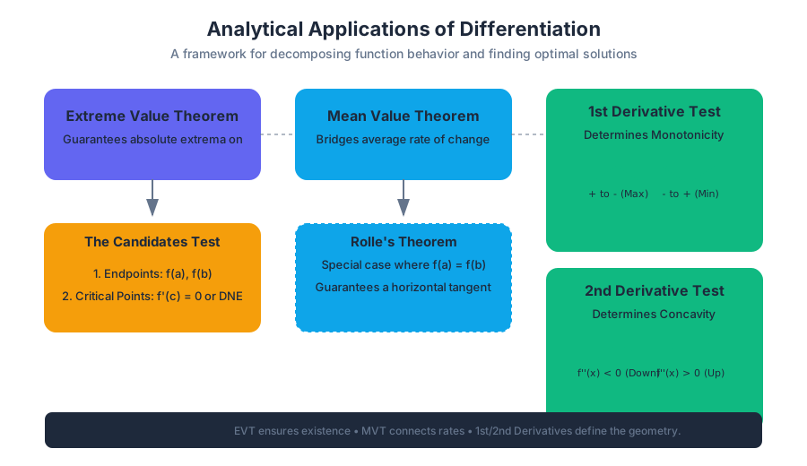
Integration and Accumulation of Change
Key concepts: Definite Integrals · Fundamental Theorem of Calculus · Riemann Sums · Antidifferentiation · Accumulation Functions
Introduction to integration as the accumulation of quantities and the reverse of differentiation.
Integration and Accumulation of Change
Integration is the mathematical engine of accumulation. While differentiation allows us to zoom in on a single point to find an instantaneous rate of change, integration allows us to zoom out, aggregating those infinitesimal changes to determine a total result. It is the bridge between the local behavior of a function and its global impact. In the context of physics, if the derivative takes us from position to velocity, the integral takes us from velocity back to the total displacement.
The Foundation: Riemann Sums and Approximation
Before we can define the integral formally, we must understand the process of partitioning. A Riemann Sum is a method for approximating the total area under a curve (the accumulation of a quantity) by dividing the region into several shapes (typically rectangles) whose areas are easy to calculate.
What it is
A Riemann sum approximates the definite integral $\int_a^b f(x) , dx$ by summing the areas of $n$ rectangles. The interval $[a, b]$ is divided into $n$ subintervals of width $\Delta x = \frac{b-a}{n}$. The height of each rectangle is determined by the value of the function at a specific point $c_i$ within each subinterval.
The Four Primary Summation Types
The choice of $c_i$ determines the type of Riemann sum and the nature of its error:
| Method | Selection of $c_i$ | Geometric Interpretation | Error Characteristic |
|---|---|---|---|
| Left Riemann Sum (LRAM) | $x_{i-1}$ (Left endpoint) | Rectangles align with the start of the interval. | Underestimates if $f(x)$ is increasing; Overestimates if decreasing. |
| Right Riemann Sum (RRAM) | $x_i$ (Right endpoint) | Rectangles align with the end of the interval. | Overestimates if $f(x)$ is increasing; Underestimates if decreasing. |
| Midpoint Sum (MRAM) | $\frac{x_{i-1} + x_i}{2}$ | Rectangles align with the center of the interval. | Generally more accurate than LRAM/RRAM; balances error. |
| Trapezoidal Rule | Average of endpoints | Uses trapezoids instead of rectangles. | Overestimates if $f(x)$ is concave up; Underestimates if concave down. |
Implementation: Numerical Integration
In computational science, we rarely solve integrals analytically if the function is discrete or highly complex. Below is a low-level implementation of these summation methods.
import numpy as np

def riemann_sum(f, a, b, n, method='midpoint'):
    """
    Computes the Riemann Sum for a function f from a to b with n subintervals.

    Args:
        f: The function to integrate.
        a, b: The bounds of integration.
        n: Number of subintervals.
        method: 'left', 'right', or 'midpoint'.
    """
    dx = (b - a) / n
    x = np.linspace(a, b, n + 1)

    if method == 'left':
        sample_points = x[:-1]
    elif method == 'right':
        sample_points = x[1:]
    elif method == 'midpoint':
        sample_points = x[:-1] + dx / 2
    else:
        raise ValueError("Method must be 'left', 'right', or 'midpoint'")

    # Summation: Σ f(c_i) * Δx
    total_sum = np.sum(f(sample_points) * dx)
    return total_sum

# Example: Integrate f(x) = x^2 from 0 to 1 with 1000 bins
f_x = lambda x: x**2
result = riemann_sum(f_x, 0, 1, 1000, method='midpoint')
print(f"Approximated Integral: {result:.6f}") # Expected near 0.333333
The Definite Integral
The Definite Integral is the limit of the Riemann sum as the number of subintervals $n$ approaches infinity (and the width $\Delta x$ approaches zero).
Mathematical Definition
The Definite Integral: Let $f$ be a function defined on $[a, b]$. If the limit exists, the definite integral of $f$ from $a$ to $b$ is: $$\int_a^b f(x) , dx = \lim_{n \to \infty} \sum_{i=1}^n f(c_i) \Delta x$$ where $\Delta x = \frac{b-a}{n}$ and $c_i$ is any point in the $i$-th subinterval.
Why it Matters
The definite integral represents the net signed area between the function and the x-axis. Area above the axis is positive, while area below is negative. This distinction is vital in physics: the integral of velocity over time gives displacement (net change in position), whereas the integral of the absolute value of velocity gives total distance traveled.
Properties of Definite Integrals
Understanding the algebraic properties of integrals allows for the simplification of complex problems.
| Property | Notation | Description |
|---|---|---|
| Additivity | $\int_a^b f(x)dx + \int_b^c f(x)dx = \int_a^c f(x)dx$ | Integrals over adjacent intervals can be combined. |
| Linearity | $\int (kf(x) + g(x))dx = k\int f(x)dx + \int g(x)dx$ | Constants can be pulled out; integrals of sums are sums of integrals. |
| Reversal | $\int_a^b f(x)dx = -\int_b^a f(x)dx$ | Swapping bounds negates the result. |
| Zero Width | $\int_a^a f(x)dx = 0$ | No area exists over a single point. |
Antidifferentiation: Reversing the Derivative
To evaluate integrals without summing infinite rectangles, we use Antidifferentiation. An antiderivative $F(x)$ is a function such that $F'(x) = f(x)$.
The Indefinite Integral
The set of all antiderivatives of $f(x)$ is the Indefinite Integral, denoted as: $$\int f(x) , dx = F(x) + C$$ The Constant of Integration ($C$) is required because the derivative of any constant is zero; therefore, infinitely many functions share the same derivative.
Common Antidifferentiation Rules
\begin{aligned}
\text{Power Rule:} & \quad \int x^n \, dx = \frac{x^{n+1}}{n+1} + C \quad (n \neq -1) \\
\text{Exponential:} & \quad \int e^x \, dx = e^x + C \\
\text{Logarithmic:} & \quad \int \frac{1}{x} \, dx = \ln|x| + C \\
\text{Trigonometric:} & \quad \int \cos(x) \, dx = \sin(x) + C
\end{aligned}
The Fundamental Theorem of Calculus (FTC)
The Fundamental Theorem of Calculus is the "Great Unification" of mathematics. It links the concept of the derivative (slope) with the integral (area).
FTC Part 1: The Accumulation Function
The first part of the theorem states that if we define a function based on the area accumulating under another function, the rate at which that area grows is exactly the value of the original function.
FTC Part 1: If $f$ is continuous on $[a, b]$ and $g(x) = \int_a^x f(t) , dt$, then: $$g'(x) = f(x)$$
This implies that integration and differentiation are inverse processes. If you integrate a function and then differentiate the result, you return to the starting function.
FTC Part 2: The Evaluation Theorem
The second part provides a practical tool for calculating definite integrals using antiderivatives, removing the need for limits of Riemann sums.
FTC Part 2: If $f$ is continuous on $[a, b]$ and $F$ is any antiderivative of $f$, then: $$\int_a^b f(x) , dx = F(b) - F(a)$$
Derivation of FTC Part 1
To understand why the derivative of an accumulation function is the function itself, consider the definition of the derivative:
Let g(x) = ∫[a to x] f(t) dt.
By definition:
g'(x) = lim(h→0) [g(x + h) - g(x)] / h

Substitute the integral definition:
g'(x) = lim(h→0) [∫[a to x+h] f(t) dt - ∫[a to x] f(t) dt] / h

Using the property of additivity:
g'(x) = lim(h→0) [∫[x to x+h] f(t) dt] / h

By the Mean Value Theorem for Integrals, there exists a c in [x, x+h] such that:
∫[x to x+h] f(t) dt = f(c) * h

Substitute back:
g'(x) = lim(h→0) [f(c) * h] / h = lim(h→0) f(c)

As h → 0, c must approach x. Since f is continuous:
g'(x) = f(x)
Accumulation Functions in Context
Accumulation functions are not just abstract constructs; they model real-world systems where a "stock" is affected by a "flow."
- Physics (Kinematics): Position $s(x)$ is the accumulation of velocity $v(t)$. $s(x) = \int_0^x v(t) , dt + s(0)$.
- Engineering (Hydrology): The total volume of water in a reservoir is the integral of the flow rate (inflow minus outflow).
- Economics: Total cost is the accumulation of marginal cost.
Real-World Example: Energy Consumption
Suppose a sensor records the power consumption of a factory in kilowatts (kW) over 24 hours. To find the total energy used in kilowatt-hours (kWh), we must integrate the power function.
from scipy.integrate import quad

# Power function P(t) in kW, where t is hours since midnight
# P(t) = 10 + 5*sin(π*t/12) + 0.5*t
def power_usage(t):
    return 10 + 5 * np.sin(np.pi * t / 12) + 0.5 * t

# Calculate total energy (kWh) over 24 hours
total_energy, error = quad(power_usage, 0, 24)

print(f"Total Energy Consumed: {total_energy:.2f} kWh")
# The 'quad' function uses adaptive quadrature to solve the integral
Advanced Variations: Integration by Substitution
When an integral involves a composite function, we use u-substitution, which is essentially the Chain Rule in reverse.
The Mechanics of u-Substitution
- Identify an "inner" function $u = g(x)$ whose derivative $du = g'(x)dx$ is also present in the integrand.
- Substitute $u$ and $du$ into the integral.
- Change the bounds of integration (for definite integrals) to correspond to $u$.
- Integrate with respect to $u$.
- Substitute back or evaluate.
Example: Evaluate $\int_0^2 2x e^{x^2} , dx$
- Let $u = x^2$. Then $du = 2x , dx$.
- When $x=0, u=0$. When $x=2, u=4$.
- The integral becomes $\int_0^4 e^u , du = [e^u]_0^4 = e^4 - e^0 = e^4 - 1$.
Common Pitfalls and Misconceptions
| Pitfall | Explanation | Correction |
|---|---|---|
| Forgetting $+ C$ | In indefinite integrals, the constant is required to represent the family of functions. | Always add $+ C$ unless it is a definite integral. |
| Area vs. Net Change | $\int f(x)dx$ calculates signed area. If the curve is below the x-axis, it subtracts from the total. | To find "Total Area," integrate $ |
| Improper Bounds | Using $x$-bounds after substituting for $u$. | Either substitute back to $x$ at the end or update the bounds to $u$-values immediately. |
| Discontinuities | FTC requires the function to be continuous on $[a, b]$. | If $f(x)$ has a vertical asymptote (e.g., $1/x^2$ at $x=0$), the integral is "improper" and requires limits. |
Summary of Integration Techniques
To master accumulation, one must choose the right tool for the specific mathematical structure of the problem.
| Structure | Recommended Technique |
|---|---|
| Polynomials / Simple Powers | Power Rule ($\frac{x^{n+1}}{n+1}$) |
| Composite Functions ($f(g(x))g'(x)$) | u-Substitution |
| Products of Functions ($u \cdot v'$) | Integration by Parts (Inverse of Product Rule) |
| Rational Functions | Partial Fraction Decomposition |
| Discrete Data Points | Trapezoidal Rule or Simpson's Rule |
Final Insight for the Practitioner
Integration is the mathematical embodiment of "the whole is the sum of its parts." Whether you are a civil engineer calculating the stress accumulation on a bridge, a data scientist determining the cumulative distribution function of a dataset, or a physicist modeling the path of a particle, the principles of Riemann sums and the Fundamental Theorem of Calculus provide the rigorous framework necessary to move from instantaneous observations to total, accumulated truth.
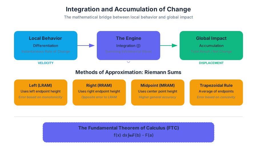
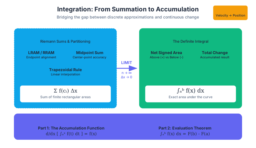
Differential Equations and Modeling
Key concepts: Slope Fields · Separation of Variables · General vs. Particular Solutions · Exponential Growth and Decay · Initial Conditions
Solving equations that involve derivatives and modeling growth and decay.
Differential Equations and Modeling
In the study of calculus, we often focus on the relationship between a function and its instantaneous rate of change. However, in the real world—from the cooling of a cup of coffee to the spread of a viral pathogen—we rarely start with a clean function. Instead, we start with a relationship: an observation of how a system changes relative to its current state. This is the domain of Differential Equations (DEs).
A differential equation is, at its simplest, an equation involving a function and one or more of its derivatives. Solving a differential equation means finding the original function (or family of functions) that satisfies the stated relationship. This section explores the visual, analytical, and modeling techniques required to navigate these foundational tools of modern science and engineering.
The Anatomy of Differential Equations
Before diving into solutions, we must categorize the types of equations we encounter. In a first-year calculus context, we primarily focus on First-Order Ordinary Differential Equations (ODEs). These involve only the first derivative, $dy/dx$, and a single independent variable.
General vs. Particular Solutions
When we integrate a differential equation, we introduce a constant of integration, $C$. This results in a General Solution, which represents an infinite family of curves. Each curve in the family shares the same derivative property but is shifted or scaled.
To narrow this down to a single, unique curve, we require an Initial Condition—a specific point $(x_0, y_0)$ through which the solution must pass. Applying this condition allows us to solve for $C$, yielding the Particular Solution.
| Concept | Definition | Mathematical Form | Result Type |
|---|---|---|---|
| Differential Equation | An equation relating $y, x,$ and $dy/dx$. | $dy/dx = f(x, y)$ | A relationship |
| General Solution | The set of all possible functions satisfying the DE. | $y = g(x) + C$ | A family of curves |
| Initial Condition | A known point on the solution curve. | $y(x_0) = y_0$ | A constraint |
| Particular Solution | The specific function satisfying both the DE and the initial condition. | $y = g(x) + 5$ | A single curve |
The Existence and Uniqueness Theorem: For a first-order DE $dy/dx = f(x, y)$, if $f$ and its partial derivative with respect to $y$ are continuous near a point $(x_0, y_0)$, then there exists a unique particular solution passing through that point.
Slope Fields: Visualizing the Derivative
When an analytical solution is difficult or impossible to find, we turn to qualitative analysis. A Slope Field (or direction field) is a graphical representation of a differential equation. Since $dy/dx$ represents the slope of the tangent line at any point $(x, y)$, we can draw short line segments at various points in the Cartesian plane to visualize the "flow" of the solutions.
Construction and Interpretation
To construct a slope field for $dy/dx = f(x, y)$:
- Select a grid of points $(x, y)$.
- Calculate the value of the derivative at each point.
- Draw a short line segment with that calculated slope at each point.
By looking at a slope field, we can identify Equilibrium Solutions (where $dy/dx = 0$), see where solutions are increasing or decreasing, and observe the Concavity of the solution curves.
Implementation: Generating Slope Fields
In professional engineering contexts, we use computational tools to generate these fields to identify stability regions in dynamical systems.
import numpy as np
import matplotlib.pyplot as plt

def plot_slope_field(f, x_range, y_range, density=20):
    """
    Plots a slope field for a given differential equation dy/dx = f(x, y).
    """
    x = np.linspace(x_range[0], x_range[1], density)
    y = np.linspace(y_range[0], y_range[1], density)
    X, Y = np.meshgrid(x, y)

    # Calculate slopes
    U = 1.0
    V = f(X, Y)

    # Normalize vectors for uniform appearance
    N = np.sqrt(U**2 + V**2)
    U /= N
    V /= N

    plt.figure(figsize=(8, 6))
    plt.quiver(X, Y, U, V, color='blue', alpha=0.6, pivot='mid')
    plt.title(f"Slope Field for dy/dx")
    plt.xlabel("x")
    plt.ylabel("y")
    plt.grid(True)
    plt.show()

# Example: dy/dx = x - y
plot_slope_field(lambda x, y: x - y, [-3, 3], [-3, 3])
Separation of Variables: The Analytical Engine
Separation of Variables is the primary algebraic technique for solving first-order differential equations. It is applicable when the derivative can be expressed as a product of a function of $x$ and a function of $y$: $$\frac{dy}{dx} = g(x)h(y)$$
The Algorithm
To solve via separation, follow these rigorous steps:
| Step | Action | Mathematical Operation |
|---|---|---|
| 1 | Separate | Move all $y$ terms (including $dy$) to one side and $x$ terms (including $dx$) to the other. |
| 2 | Integrate | Perform indefinite integration on both sides. |
| 3 | Constant | Add the constant of integration $+C$ (usually on the $x$-side). |
| 4 | Solve for $y$ | Use algebra to isolate $y$ (the General Solution). |
| 5 | Apply IC | If an initial condition is given, solve for $C$ (the Particular Solution). |
Worked Example: Solving a Separable Equation
Find the particular solution for $\frac{dy}{dx} = \frac{x^2}{y}$ given the initial condition $y(0) = 2$.
\begin{aligned}
\text{1. Separate variables: } & y \, dy = x^2 \, dx \\
\text{2. Integrate both sides: } & \int y \, dy = \int x^2 \, dx \\
\text{3. Result of integration: } & \frac{1}{2}y^2 = \frac{1}{3}x^3 + C \\
\text{4. Solve for General Solution: } & y^2 = \frac{2}{3}x^3 + C_1 \implies y = \pm\sqrt{\frac{2}{3}x^3 + C_1} \\
\text{5. Apply Initial Condition } (0, 2): & 2 = \sqrt{\frac{2}{3}(0)^3 + C_1} \implies 2 = \sqrt{C_1} \implies C_1 = 4 \\
\text{6. Particular Solution: } & y = \sqrt{\frac{2}{3}x^3 + 4}
\end{aligned}
Warning: Always add the constant $C$ immediately after integrating. Adding it at the very end of the algebraic manipulation is a common error that leads to incorrect particular solutions.
Exponential Growth and Decay Models
One of the most significant applications of differential equations is modeling quantities that change at a rate proportional to their current size. This is described by the equation: $$\frac{dy}{dt} = ky$$ where $k$ is the growth constant ($k > 0$) or decay constant ($k < 0$).
Derivation of the Law of Exponential Change
We can derive the standard growth formula using separation of variables:
DERIVATION: dy/dt = ky
-----------------------
1. Separate: (1/y) dy = k dt
2. Integrate: ∫ (1/y) dy = ∫ k dt
3. Compute: ln|y| = kt + C
4. Exponentiate: |y| = e^(kt + C)
5. Simplify: |y| = e^C * e^(kt)
6. Let A = ±e^C: y(t) = A * e^(kt)

At t=0, y(0) = A * e^0 = A.
Therefore, A is the initial amount (y₀).

FINAL FORM: y(t) = y₀ * e^(kt)
Real-World Applications
Exponential models appear across diverse fields. The behavior is determined entirely by the sign and magnitude of $k$.
| Application | Equation Variant | Context |
|---|---|---|
| Population Growth | $dP/dt = kP$ | Unconstrained biological growth. |
| Radioactive Decay | $dm/dt = -km$ | The rate of decay is proportional to the mass remaining. |
| Newton's Law of Cooling | $dT/dt = -k(T - T_s)$ | Rate of temp change is proportional to the difference with surroundings. |
| Continuous Interest | $dA/dt = rA$ | Financial modeling of continuously compounded accounts. |
Newton's Law of Cooling: A Case Study
Newton's Law of Cooling states that the rate of change of the temperature $T$ of an object is proportional to the difference between its temperature and the ambient temperature $T_s$. $$\frac{dT}{dt} = -k(T - T_s)$$ This is a separable DE. If we let $u = T - T_s$, then $du/dt = dT/dt$, and the equation simplifies to $du/dt = -ku$, which we already know results in $u(t) = u_0 e^{-kt}$. Substituting back: $$T(t) = T_s + (T_0 - T_s)e^{-kt}$$
Numerical Methods: When Algebra Fails
Not all differential equations are separable. For equations like $dy/dx = x + y$, we cannot isolate variables. In these cases, we use numerical approximation. The most fundamental method is Euler's Method.
Euler's Method uses the slope at a point to predict the next point a small distance $\Delta x$ (step size $h$) away. $$y_{n+1} = y_n + f(x_n, y_n) \cdot h$$
# Example of using a CLI-based tool or script to approximate a DE solution
# Usage: ./euler_solver --equation "x+y" --x0 0 --y0 1 --step 0.1 --iterations 10

Iter 0: (0.000, 1.000)
Iter 1: (0.100, 1.100) # y1 = 1.0 + (0+1)*0.1
Iter 2: (0.200, 1.220) # y2 = 1.1 + (0.1+1.1)*0.1
Iter 3: (0.300, 1.362) # y3 = 1.22 + (0.2+1.22)*0.1
...
Final Approximation at x=1.0: y ≈ 3.187
Common Pitfalls and Advanced Nuances
Even experienced practitioners encounter friction when modeling with DEs. Mastery requires recognizing these subtle traps.
1. The Absolute Value Trap
When integrating $1/y$, the result is $\ln|y|$. If the initial condition $y_0$ is negative, the absolute value is crucial.
- If $y > 0$, then $y = e^{kt+C}$.
- If $y < 0$, then $y = -e^{kt+C}$. The sign of the initial condition determines which branch of the solution you are on.
2. Domain of Validity
A particular solution is only valid on the continuous interval containing the initial condition. If the solution $y(x)$ has a vertical asymptote (e.g., $y = 1/(1-x)$), and your initial condition is at $x=0$, the solution is only valid for $x < 1$.
3. Misinterpreting Slope Fields
Students often confuse the slope field of $dy/dx = f(x)$ with $dy/dx = f(y)$.
- If $dy/dx$ depends only on $x$, all segments in a vertical column are parallel.
- If $dy/dx$ depends only on $y$ (Autonomous Equation), all segments in a horizontal row are parallel.
4. The $+C$ Placement
In separation of variables, $C$ represents the accumulation of constants from both sides. It must be present before you perform algebraic operations like exponentiation or square roots.
- Correct: $\ln|y| = x + C \implies y = e^{x+C} = Ce^x$
- Incorrect: $\ln|y| = x \implies y = e^x \implies y = e^x + C$
Summary of Modeling Workflow
To model a physical system using differential equations, follow this pipeline:
- Identify the Rate: Determine what $dy/dt$ represents (e.g., velocity, rate of decay).
- Formulate the Equation: Translate the physical description into math (e.g., "rate is proportional to..." $\to dy/dt = ky$).
- Choose a Method:
- Can variables be separated? Use Separation of Variables.
- Is it a standard growth/decay model? Use $y = y_0 e^{kt}$.
- Is it complex? Use Slope Fields or Numerical Methods.
- Solve for $C$: Use the initial state of the system.
- Interpret: Ensure the limits of the function make sense (e.g., population shouldn't go to infinity if there's a carrying capacity).
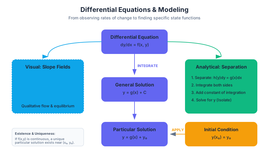
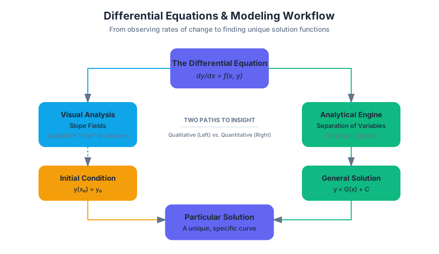
Applications of Integration: Area and Volume
Key concepts: Area Between Curves · Volumes with Cross Sections · Volumes of Revolution (Disk/Washer) · Average Value of a Function · Net Change
Using definite integrals to calculate area between curves and the volume of complex solids.
Applications of Integration: Area and Volume
In the study of calculus, the definite integral is often introduced as the "area under a curve." However, this is a pedagogical simplification. In a broader engineering and mathematical context, integration is the ultimate tool for accumulation. Whether we are accumulating distance from velocity, mass from density, or three-dimensional slices into a solid volume, the underlying principle remains the same: we partition a complex whole into infinitesimal "representative elements," model those elements, and sum them using the Fundamental Theorem of Calculus.
This article explores the rigorous application of integration to determine the geometric properties of shapes and the physical accumulation of quantities.
Net Change and the Accumulation of Quantities
The Net Change Theorem is a direct application of the Fundamental Theorem of Calculus. It states that the integral of a rate of change is the net change in the original quantity.
The Net Change Theorem: If $f'(x)$ is the rate of change of a quantity $f(x)$, then the definite integral of $f'(x)$ from $a$ to $b$ gives the total change in $f(x)$: $$\int_{a}^{b} f'(x) , dx = f(b) - f(a)$$
Displacement vs. Total Distance
One of the most critical distinctions in physics and engineering is the difference between net change (displacement) and total accumulation (total distance traveled).
| Concept | Mathematical Definition | Physical Meaning |
|---|---|---|
| Displacement | $\int_{a}^{b} v(t) , dt$ | The change in position from $t=a$ to $t=b$. |
| Total Distance | $\int_{a}^{b} | v(t) |
| Net Change | $\int_{a}^{b} r(t) , dt$ | The total increase/decrease of a quantity (e.g., water in a tank). |
Pitfall: The Sign of the Function
When calculating net change, the sign of the rate function $r(t)$ matters. If $r(t)$ represents the rate of water flowing into a tank, a negative value implies water is flowing out. To find the total amount of water processed (in and out), one must integrate the absolute value of the rate.
Average Value of a Function
In discrete mathematics, the average of $n$ numbers is their sum divided by $n$. In the continuous domain, we use integration to find the Average Value of a function over an interval $[a, b]$.
Definition: Average Value The average value of a continuous function $f(x)$ on the interval $[a, b]$ is: $$f_{avg} = \frac{1}{b-a} \int_{a}^{b} f(x) , dx$$
Geometric Interpretation
The average value $f_{avg}$ represents the height of a rectangle with the same base $(b-a)$ that would yield the exact same area as the region under the curve $f(x)$. This is deeply tied to the Mean Value Theorem for Integrals, which guarantees that for a continuous function, there exists at least one point $c$ in $[a, b]$ such as $f(c) = f_{avg}$.
# Example 1: Numerical computation of Average Value using SciPy
import numpy as np
from scipy.integrate import quad

def function_to_average(x):
    """Example function: f(x) = sin(x) + 0.5x"""
    return np.sin(x) + 0.5 * x

def calculate_average_value(func, a, b):
    # Perform numerical integration
    area, error = quad(func, a, b)
    # Divide by the interval width
    avg_val = area / (b - a)
    return avg_val

# Interval [0, 2*pi]
a, b = 0, 2 * np.pi
result = calculate_average_value(function_to_average, a, b)
print(f"The average value of the function over [{a}, {b}] is: {result:.4f}")
Area Between Curves
Calculating the area between two intersecting or bounding curves is the first step in moving from "area under a curve" to "area of a region."
Vertical Slicing ($dx$)
If a region is bounded above by $f(x)$ and below by $g(x)$ over an interval $[a, b]$, the area $A$ is found by integrating the "height" of a representative vertical rectangle: $$A = \int_{a}^{b} [f(x) - g(x)] , dx$$
Horizontal Slicing ($dy$)
In cases where functions are defined in terms of $y$, or where the boundaries change vertically, it is often more efficient to integrate with respect to $y$. If a region is bounded on the right by $x = f(y)$ and on the left by $x = g(y)$ from $y = c$ to $y = d$: $$A = \int_{c}^{d} [f(y) - g(y)] , dy$$
Comparison of Slicing Orientations
| Feature | Vertical Slicing ($dx$) | Horizontal Slicing ($dy$) |
|---|---|---|
| Representative Element | Vertical rectangle | Horizontal rectangle |
| Height/Width | $f(x) - g(x)$ (Top - Bottom) | $f(y) - g(y)$ (Right - Left) |
| Integration Limits | $x$-coordinates of boundaries | $y$-coordinates of boundaries |
| Best Used When... | Boundaries are $y = \dots$ | Boundaries are $x = \dots$ |
Volumes with Known Cross Sections
Before moving to solids of revolution, we must understand the general principle of volume: the integral of the cross-sectional area. If a solid has a base in the $xy$-plane and every cross-section perpendicular to the $x$-axis has a known area $A(x)$, the volume $V$ is: $$V = \int_{a}^{b} A(x) , dx$$
Common Cross-Sectional Geometries
The challenge in these problems is usually not the integration itself, but expressing the area $A(x)$ in terms of the side length $s$, which is determined by the distance between two curves $f(x)$ and $g(x)$.
| Cross-Section Shape | Area Formula $A(s)$ | $s$ in terms of curves |
|---|---|---|
| Square | $s^2$ | $f(x) - g(x)$ |
| Semicircle | $\frac{1}{8}\pi s^2$ | $f(x) - g(x)$ |
| Equilateral Triangle | $\frac{\sqrt{3}}{4} s^2$ | $f(x) - g(x)$ |
| Isosceles Rt. Triangle (Leg on base) | $\frac{1}{2} s^2$ | $f(x) - g(x)$ |
\text{Derivation of the Volume of a Pyramid with height } H \text{ and base area } B: \\
\text{By similar triangles, the side length } s \text{ at height } h \text{ is } s(h) = \sqrt{B} \frac{H-h}{H}. \\
\text{The area of the cross-section is } A(h) = s(h)^2 = B \frac{(H-h)^2}{H^2}. \\
V = \int_{0}^{H} B \frac{(H-h)^2}{H^2} dh = \frac{B}{H^2} \left[ -\frac{(H-h)^3}{3} \right]_{0}^{H} = \frac{1}{3}BH.
Volumes of Revolution: The Disk Method
When a two-dimensional region is rotated around an axis, it creates a three-dimensional solid. If the region is flush against the axis of rotation, we use the Disk Method.
Mechanics
Imagine a thin vertical rectangle of width $dx$ and height $R(x)$ being rotated around the $x$-axis. It forms a thin cylinder (a disk) with:
- Radius: $R(x)$
- Volume of one disk: $dV = \pi [R(x)]^2 dx$
Summing these disks from $a$ to $b$ gives the total volume: $$V = \pi \int_{a}^{b} [R(x)]^2 , dx$$
Rotation around the y-axis
If the region is rotated around the $y$-axis and bounded by $x = R(y)$, the formula becomes: $$V = \pi \int_{c}^{d} [R(y)]^2 , dy$$
Volumes of Revolution: The Washer Method
If there is a "gap" between the region and the axis of rotation, the resulting solid will have a hole in the middle. The cross-section perpendicular to the axis is a washer (an annulus).
The Formula
To find the volume, we subtract the volume of the inner "empty" solid from the volume of the outer "full" solid. $$V = \pi \int_{a}^{b} \left( [R_{out}(x)]^2 - [R_{in}(x)]^2 \right) , dx$$ Where:
- $R_{out}(x)$ is the distance from the axis to the outer curve.
- $R_{in}(x)$ is the distance from the axis to the inner curve.
Critical Warning: A common error is to write $\pi \int (R_{out} - R_{in})^2 dx$. This is algebraically incorrect. You must square the radii individually: $R_{out}^2 - R_{in}^2$.
Example: Rotating around a non-axis line
Suppose we rotate the region between $y = x^2$ and $y = x$ around the line $y = -1$.
- Outer Radius: $R_{out} = x - (-1) = x + 1$
- Inner Radius: $R_{in} = x^2 - (-1) = x^2 + 1$
- Integral: $V = \pi \int_{0}^{1} [(x+1)^2 - (x^2+1)^2] , dx$
# Using SymPy (Python library) via CLI to solve the Washer Method problem
# Problem: Rotate y=x and y=x^2 around y=-1 from x=0 to x=1
python3 -c "
import sympy as sp
x = sp.Symbol('x')
R_out = x + 1
R_in = x**2 + 1
volume = sp.pi * sp.integrate(R_out**2 - R_in**2, (x, 0, 1))
print(f'Exact Volume: {volume}')
print(f'Decimal: {volume.evalf()}')
"
Summary of Volume Methods
Choosing the correct method is often the most difficult part of an integration problem. The following table serves as a decision matrix for volume problems.
| Method | When to Use | Representative Element | Integral Setup |
|---|---|---|---|
| Cross-Sections | Solid built on a base with known shapes | Slabs of thickness $dx$ | $\int A(x) dx$ |
| Disk Method | Rotation around axis, no gap | Solid disk | $\pi \int [R(x)]^2 dx$ |
| Washer Method | Rotation around axis, with gap | Hollow washer | $\pi \int (R_{out}^2 - R_{in}^2) dx$ |
| Shell Method* | Rotation where slicing is parallel to axis | Cylindrical shell | $2\pi \int r \cdot h , dx$ |
*Note: The Shell Method is typically covered in Calculus BC or second-semester college calculus, but it is a powerful alternative when the Washer Method leads to difficult algebra.
Common Pitfalls and Expert Tips
- Incorrect Bounds: Always solve for the intersection points of the curves ($f(x) = g(x)$) to find your limits of integration. Do not rely solely on a visual sketch.
- The "Square of the Difference" Fallacy: In the washer method, remember that $(R_{out} - R_{in})^2 \neq R_{out}^2 - R_{in}^2$. The geometry requires the difference of the areas of two circles.
- Axis Shifts: When rotating around a line like $x = k$ or $y = k$, the radius is always $| \text{curve} - \text{axis} |$. If the axis is $y=5$ and the curve is $y=x^2$, the radius is $5 - x^2$ (if the curve is below the axis).
- Variable Mismatch: If you are rotating around a horizontal line (like the $x$-axis), your integral should usually be in terms of $x$ (for Disk/Washer). If rotating around a vertical line, use $y$.
# Advanced: Handling multiple intersection points and area accumulation
def calculate_complex_area(f, g, x_range):
    """
    Calculates the total area between two functions,
    accounting for cases where they cross each other.
    """
    # Find the absolute difference to ensure positive area
    diff_func = lambda x: abs(f(x) - g(x))

    total_area, error = quad(diff_func, x_range[0], x_range[1])
    return total_area

# Example: f(x) = sin(x), g(x) = cos(x) from 0 to pi
import math
f = math.sin
g = math.cos
area = calculate_complex_area(f, g, [0, math.pi])
print(f"Total area between sin(x) and cos(x) on [0, pi]: {area:.4f}")
Conclusion
The applications of integration to area and volume represent a transition from purely algebraic manipulation to spatial reasoning. By conceptualizing a volume as an infinite sum of infinitesimal area slices, we gain the ability to model everything from the capacity of a fuel tank to the mass distribution of a planetary body. Mastery of these techniques requires a dual focus: the geometric intuition to set up the "representative element" and the technical precision to evaluate the resulting definite integral.
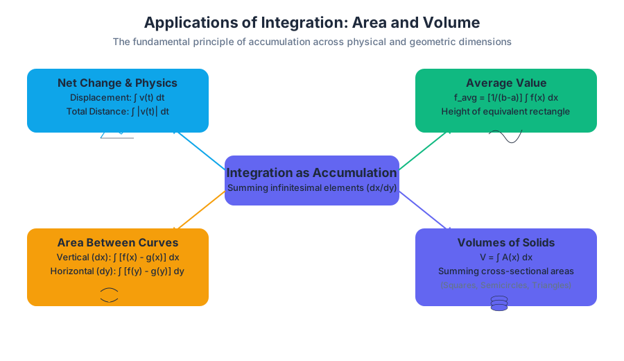
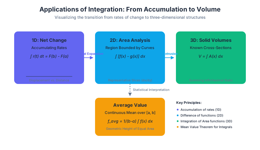
AP Calculus AB Exam Preparation
Key concepts: Free Response Questions (FRQs) · Step-by-step Problem Solving · Scoring Rubrics · Past Exam Analysis (2011, 2015, 2017)
Reviewing past Free Response Questions (FRQs) and mastering exam-taking strategies.
AP Calculus AB Exam Preparation
The AP Calculus AB exam represents the culmination of a rigorous study of single-variable calculus, focusing on limits, derivatives, integrals, and the Fundamental Theorem of Calculus. Success on this assessment requires more than mere computational fluency; it demands a high level of conceptual synthesis and the ability to communicate mathematical reasoning with precision. The exam is divided into two primary sections: Multiple Choice Questions (MCQ) and Free Response Questions (FRQ). While the MCQ tests breadth of knowledge, the FRQ section evaluates the depth of a student’s ability to model real-world scenarios, justify conclusions using named theorems, and navigate the interplay between analytical, graphical, and tabular representations.
The Architecture of the Free Response Question (FRQ)
The FRQ section consists of six questions, each worth nine points, for a total of 54 points (weighted as 50% of the total exam score). These questions are split into two parts:
- Part A (Questions 1–2): Graphing calculator required. These problems often involve complex functions where manual integration or root-finding is impractical.
- Part B (Questions 3–6): No calculator permitted. These problems focus on symbolic manipulation, theorem application, and interpreting graphs or tables.
The Scoring Rubric Philosophy
The College Board employs a "point-stacking" rubric. Points are typically awarded for the setup (the definite integral or derivative expression), the intermediate steps (applying a rule or theorem), and the final answer (with correct units). A "bald answer"—an answer provided without supporting work—usually earns zero points, even if correct.
| Point Category | Requirement | Common Pitfall |
|---|---|---|
| Setup/Expression | Writing the integral or derivative with correct limits/variables. | Forgetting $dx$ or $dt$ in the integral. |
| Computation | Correct application of Power Rule, Chain Rule, or FTC. | Arithmetic errors in simple subtraction. |
| Justification | Verbal explanation using a named theorem (MVT, IVT, EVT). | Using "it" instead of the function name (e.g., "$f(x)$ increases"). |
| Units of Measure | Correct units (e.g., $ft/sec^2$ for acceleration). | Omitting units when specifically asked. |
Core Competencies in Problem Solving
To master the FRQ, a student must internalize the "Big Four" concepts: Limits/Continuity, Differentiation, Integration, and Differential Equations. Each of these is tested through specific lenses, such as Rate In/Rate Out problems or Particle Motion.
1. Numerical Integration and Riemann Sums
Often appearing in tabular problems, students must approximate the area under a curve using Left, Right, Midpoint, or Trapezoidal sums. This tests the understanding of the definite integral as an accumulation of change.
# Low-level implementation of a Trapezoidal Riemann Sum
# Used to approximate the definite integral of a function given as discrete data points

def trapezoidal_rule(x_coords, y_coords):
    """
    Calculates the area under the curve using the trapezoidal rule.
    x_coords: List of time/position values (must be strictly increasing)
    y_coords: List of function values at those points
    """
    if len(x_coords) != len(y_coords):
        raise ValueError("Data point mismatch: x and y must have same length.")

    total_area = 0.0
    for i in range(len(x_coords) - 1):
        # Width of the sub-interval
        dx = x_coords[i+1] - x_coords[i]
        # Average height of the trapezoid
        avg_height = (y_coords[i] + y_coords[i+1]) / 2.0
        total_area += dx * avg_height

    return total_area

# Example usage from a 2017-style table problem
time_points = [0, 2, 5, 10]
velocity_points = [0, 15, 20, 30]
print(f"Total Displacement: {trapezoidal_rule(time_points, velocity_points)} units")
2. The Fundamental Theorem of Calculus (FTC)
The FTC is the bridge between the derivative and the integral. In FRQs, this often appears in the form of a "Function Defined by an Integral":
$g(x) = \int_{a}^{x} f(t) dt$
Students must recognize that $g'(x) = f(x)$ and $g''(x) = f'(x)$. This allows for the analysis of $g(x)$ (extrema, concavity) based solely on the graph of $f(t)$.
\text{Fundamental Theorem of Calculus (Part 1):} \\
\frac{d}{dx} \left[ \int_{a}^{g(x)} f(t) \, dt \right] = f(g(x)) \cdot g'(x) \\
\\
\text{Fundamental Theorem of Calculus (Part 2):} \\
\int_{a}^{b} f'(x) \, dx = f(b) - f(a)
Historical Analysis: Patterns in Past Exams
Analyzing past exams reveals a high degree of consistency in question types. By categorizing problems from 2011, 2015, and 2017, we can identify the "standard templates" used by the College Board.
2011 Exam: Focus on Particle Motion and Area/Volume
The 2011 exam featured a classic Particle Motion problem (Question 1). These problems require navigating between position $s(t)$, velocity $v(t)$, and acceleration $a(t)$ using differentiation and integration.
- Key Insight: "Total Distance" is $\int |v(t)| dt$, whereas "Displacement" is $\int v(t) dt$.
2015 Exam: Rate In/Rate Out and Accumulation
Question 1 of the 2015 exam (the "Drainage Pipe" problem) is a quintessential Rate In/Rate Out problem.
- The Model: $A(t) = A(0) + \int_{0}^{t} (\text{RateIn} - \text{RateOut}) dx$.
- Common Error: Forgetting the initial condition $A(0)$.
2017 Exam: Tabular Analysis and Differential Equations
The 2017 exam (Question 4) used a table representing the height of a tree over time. Students were asked to estimate $H'(6)$ using a difference quotient: $H'(6) \approx \frac{H(7) - H(5)}{7 - 5}$.
| Year | Problem Type | Core Concept | Calculator? |
|---|---|---|---|
| 2011 | Area/Volume | Revolving around a line (Disk/Washer Method) | Yes |
| 2015 | Accumulation | Rate of water flow into a pipe | Yes |
| 2017 | Diff. Equations | Separation of Variables: $\frac{dy}{dt} = \frac{1}{4}(10-y)$ | No |
| Common | Graph Analysis | Interpreting $f'$ to find extrema of $f$ | No |
Step-by-Step Problem Solving Strategy
When approaching an FRQ, a systematic pipeline ensures that no "easy" points are left on the table.
Phase 1: Decoding the Prompt
Identify the "Given" and the "Goal." If the prompt provides $f'(x)$ and asks for the maximum of $f(x)$, you are immediately in the territory of the Extreme Value Theorem (EVT).
Phase 2: The Setup
Write the calculus expression before plugging in numbers.
- Example: If asked for the average value of $f(x)$ on $[2, 5]$, write $\frac{1}{5-2} \int_{2}^{5} f(x) dx$.
Phase 3: Execution and Justification
Use formal language. Avoid vague pronouns.
- Incorrect: "The graph goes up so it's a max."
- Correct: "Since $f'(x)$ changes from positive to negative at $x=3$, $f(x)$ has a relative maximum at $x=3$ by the First Derivative Test."
Phase 4: Calculator Integration (Part A Only)
In the calculator section, you are expected to use the device for four specific tasks:
- Plotting a function in a meaningful window.
- Finding the roots of a function (solving $f(x) = 0$).
- Calculating the numerical derivative at a point.
- Calculating a definite integral.
# Example: Using a CLI-based math tool (like 'bc' or a python-shell)
# to verify a definite integral for a 2015 FRQ-style problem.
# Problem: Integrate (20 + 15*sin(pi*t/12)) from t=0 to t=8

echo "scale=5; s = 0; for(t=0; t<=8; t+=0.001) s += (20 + 15*sin(3.14159*t/12))*0.001; s" | bc -l

# Expected Output: ~220.704
Advanced Topic: Differential Equations and Separation of Variables
A staple of the non-calculator section (Part B) is the Separable Differential Equation. Students are given $\frac{dy}{dx} = f(x)g(y)$ and an initial condition $(x_0, y_0)$.
The Algorithmic Approach:
- Separate: Move all $y$ terms to the $dy$ side and $x$ terms to the $dx$ side.
- Integrate: Take the antiderivative of both sides. Do not forget $+C$.
- Solve for C: Use the initial condition immediately after integrating.
- Isolate y: Solve the resulting algebraic equation for $y$.
Theorem: Existence and Uniqueness If $f(x,y)$ and $\frac{\partial f}{\partial y}$ are continuous in a region, then there exists a unique solution to the differential equation passing through a given point in that region. In AP Calculus AB, we focus on finding this unique particular solution.
Common Pitfalls and Error Mitigation
Even high-performing students lose points to "linkage errors" and "over-rounding."
- Linkage Errors: Writing $f(x) = f'(x) = 3$. This is mathematically false and results in a point deduction for "communication."
- Rounding: Never round intermediate steps. Keep at least 6 decimal places in your calculator and only round the final answer to three decimal places (the AP standard).
- Initial Conditions: In accumulation problems (Rate In/Rate Out), students often calculate the net change $\int R(t) dt$ but forget to add the starting amount $S(0)$.
- Chain Rule Neglect: When integrating via u-substitution or differentiating composite functions, failing to account for the "inner" derivative is the most common source of algebraic error.
Comparative Analysis: Mean Value Theorem vs. Intermediate Value Theorem
| Feature | Intermediate Value Theorem (IVT) | Mean Value Theorem (MVT) |
|---|---|---|
| Prerequisite | $f(x)$ is continuous on $[a, b]$. | $f(x)$ is continuous on $[a, b]$ AND differentiable on $(a, b)$. |
| Guarantees... | A y-value (output) exists between $f(a)$ and $f(b)$. | A slope (derivative) exists equal to the average rate of change. |
| Equation | $f(c) = k$ | $f'(c) = \frac{f(b) - f(a)}{b - a}$ |
| Use Case | Proving a function has a zero (root). | Proving a car reached a specific speed. |
Final Preparation Checklist
As the exam approaches, focus on the "Justification Phrases" that graders look for. Memorize the conditions for each theorem. For example, you cannot use the Mean Value Theorem unless you explicitly state that the function is continuous and differentiable.
- Review the "Big Three" 2017 FRQs: Specifically the tree height (table), the tank volume (calculator), and the slope field (differential equations).
- Practice "Calculator Fluency": Ensure you can find intersections and integrals on your device in under 30 seconds.
- Units, Units, Units: Every time you see a "Rate" question, check if the answer requires units. If the question asks for "Rate of change of the rate of change," your units should be squared (e.g., $m/s^2$).
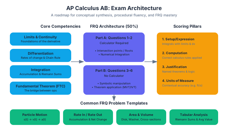
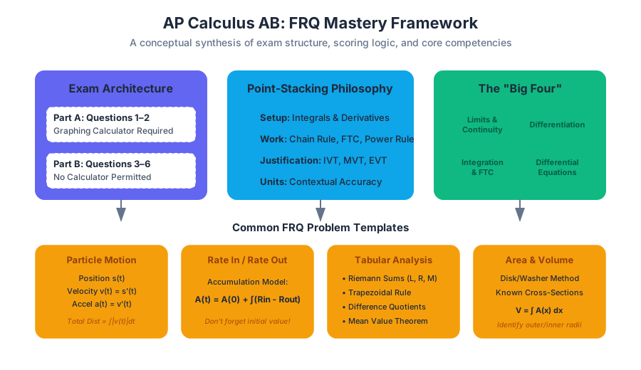
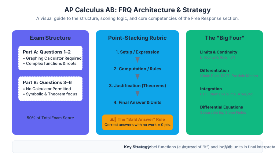
Course Challenge and Mastery
Key concepts: Mastery Points · Comprehensive Skill Assessment · Problem Solving Speed
A final assessment to test mastery of all AP Calculus AB units.
Course Challenge and Mastery
The Course Challenge represents the terminal phase of the pedagogical lifecycle in the AP Calculus AB curriculum. It is a high-fidelity, cumulative assessment designed to measure a learner's Latent Knowledge State across the entire spectrum of calculus—from the foundational epsilon-delta intuition of limits to the complex geometric rotations of solid volumes. Unlike modular unit tests, the Course Challenge serves as a "stress test" for cognitive retrieval, forcing the brain to switch contexts rapidly between disparate mathematical domains.
The Architecture of Mastery
In a modern digital learning environment, Mastery is not a binary state of "pass" or "fail." Instead, it is a quantified metric of proficiency, often represented by Mastery Points. These points act as a proxy for a student's probability of correctly solving a problem within a specific skill node under varying conditions.
Mastery Points and the Knowledge Graph
Each unit in the Calculus AB course—such as Differentiation Rules or Applications of Integration—is decomposed into granular skills. Mastery Points are accumulated through a tiered progression:
- Attempted: The learner has engaged with the material.
- Familiar: Initial correct responses in a controlled environment (Quizzes).
- Proficient: Consistent accuracy across multiple sessions (Unit Tests).
- Mastered: Successful retrieval during cumulative assessments (Course Challenge).
Definition: The Mastery Coefficient The Mastery Coefficient ($\mathcal{M}$) can be modeled as a function of accuracy ($a$), consistency over time ($t$), and the difficulty of the assessment context ($d$). Formally: $$\mathcal{M} = \int_{0}^{T} \frac{a(t) \cdot d(t)}{e^{-\lambda t}} dt$$ where $\lambda$ represents the decay constant of human forgetting (the Ebbinghaus curve).
Comparison of Assessment Tiers
| Feature | Quiz | Unit Test | Course Challenge |
|---|---|---|---|
| Scope | 2–3 specific skills | Single Unit (e.g., Integration) | Entire Curriculum (Units 1–10) |
| Question Count | 5–10 | 9–15 | 30 |
| Context Switching | Low | Moderate | High |
| Mastery Ceiling | Proficient | Proficient | Mastered |
| Time Pressure | Minimal | Moderate | Significant (30–45 mins) |
Comprehensive Skill Assessment: The 30-Question Gauntlet
The Course Challenge utilizes a 30-question heuristic to sample the vast state-space of the AP Calculus AB curriculum. To achieve statistical significance in assessing a student's readiness, the challenge must balance breadth (covering all 10 units) with depth (testing high-level synthesis).
The Distribution Logic
The assessment engine typically distributes questions according to the weighting of the AP Exam. A standard Course Challenge distribution might look like this:
| Unit ID | Topic Area | Question Weight | Key Concepts Tested |
|---|---|---|---|
| U1 | Limits & Continuity | 10% | IVT, Squeeze Theorem, Asymptotes |
| U2-U4 | Differentiation | 30% | Chain Rule, Implicit, Inverse Trig |
| U5-U6 | Analytical Apps of Derivatives | 20% | MVT, Optimization, Concavity |
| U7-U8 | Integration & Diff. Equations | 25% | Separation of Variables, FTC |
| U9-U10 | Applications of Integration | 15% | Disk/Washer Method, Area between curves |
Technical Implementation: The Mastery Update Algorithm
From a systems engineering perspective, updating a student's mastery after a Course Challenge requires a robust algorithm that accounts for prior knowledge. We do not simply add points; we adjust the confidence interval of the student's proficiency.
# Low-level implementation of a Mastery Update Engine
# Based on a simplified Bayesian Knowledge Tracing (BKT) model

class MasterySystem:
    def __init__(self, initial_p_mastery=0.1):
        self.p_m = initial_p_mastery  # Probability student knows the skill
        self.p_s = 0.1                # Probability of a 'slip' (knows it, but gets it wrong)
        self.p_g = 0.2                # Probability of a 'guess' (doesn't know, but gets it right)
        self.p_t = 0.25               # Probability of transition to mastery after practice

    def update_mastery(self, is_correct):
        if is_correct:
            # Probability they knew it given a correct answer
            p_known_given_correct = (self.p_m * (1 - self.p_s)) / \
                                    ((self.p_m * (1 - self.p_s)) + ((1 - self.p_m) * self.p_g))
            self.p_m = p_known_given_correct + (1 - p_known_given_correct) * self.p_t
        else:
            # Probability they knew it given an incorrect answer
            p_known_given_incorrect = (self.p_m * self.p_s) / \
                                      ((self.p_m * self.p_s) + ((1 - self.p_m) * (1 - self.p_g)))
            self.p_m = p_known_given_incorrect + (1 - p_known_given_incorrect) * self.p_t

        return round(self.p_m * 100, 2)

# Example: Student takes the Course Challenge and gets a Chain Rule problem correct
mastery_engine = MasterySystem(initial_p_mastery=0.5)
new_score = mastery_engine.update_mastery(is_correct=True)
print(f"Updated Mastery Probability: {new_score}%")
Problem Solving Speed and Heuristics
In the context of the Course Challenge, Problem Solving Speed is not merely about "working fast"—it is about the transition from System 2 thinking (slow, effortful, rule-based) to System 1 thinking (fast, instinctive, pattern-based).
A senior engineer or mathematician does not "re-derive" the quotient rule every time they see a rational function; they recognize the pattern and execute the algorithm. The 30–45 minute time limit on 30 questions serves as a diagnostic for this fluency.
Heuristic: The "Disguised Derivative"
One of the most common speed-traps in the Course Challenge is the "Disguised Derivative"—a limit definition of a derivative that students often try to solve using L'Hôpital's Rule or algebraic manipulation, wasting valuable minutes.
\text{Evaluate: } \lim_{h \to 0} \frac{\sin(\frac{\pi}{3} + h) - \sin(\frac{\pi}{3})}{h}
The Slow Way (System 2):
- Recognize $0/0$ indeterminate form.
- Apply L'Hôpital's Rule.
- Differentiate numerator with respect to $h$: $\cos(\frac{\pi}{3} + h)$.
- Plug in $h=0$: $\cos(\frac{\pi}{3}) = 1/2$.
The Fast Way (System 1 - Mastery):
- Recognize the form $\lim_{h \to 0} \frac{f(x+h) - f(x)}{h}$.
- Identify $f(x) = \sin(x)$ and $x = \pi/3$.
- Recall $f'(x) = \cos(x)$.
- Result: $\cos(\pi/3) = 1/2$.
The "Mastery" level student identifies the pattern in $<3$ seconds, saving time for complex "Related Rates" or "Volume of Solids" problems.
Worked Example: The Multi-Step Integration Challenge
To demonstrate the depth of the Course Challenge, consider a problem that synthesizes Unit 7 (Differential Equations) and Unit 8 (Applications of Integration).
Problem: Find the particular solution $y = f(x)$ to the differential equation $\frac{dy}{dx} = \frac{x^2}{y}$ with the initial condition $f(0) = 2$. Then, calculate the average value of $f(x)$ on the interval $[0, 3]$.
Step 1: Separation of Variables
We must isolate $y$ and $x$ terms to integrate. $$y , dy = x^2 , dx$$ $$\int y , dy = \int x^2 , dx$$ $$\frac{1}{2}y^2 = \frac{1}{3}x^3 + C$$
Step 2: Solving for $C$ (Initial Condition)
Plug in $(0, 2)$: $$\frac{1}{2}(2)^2 = \frac{1}{3}(0)^3 + C \implies 2 = C$$ The general solution is $\frac{1}{2}y^2 = \frac{1}{3}x^3 + 2$, or $y = \sqrt{\frac{2}{3}x^3 + 4}$.
Step 3: Average Value of a Function
The average value formula is $\frac{1}{b-a} \int_{a}^{b} f(x) dx$. $$\text{Avg} = \frac{1}{3-0} \int_{0}^{3} \sqrt{\frac{2}{3}x^3 + 4} , dx$$ Note: In a Course Challenge, if this were a non-calculator section, the function would be designed for a cleaner u-substitution. If calculator-active, the student must demonstrate proficiency in numerical integration.
Common Pitfalls and Edge Cases
Even high-performing students often fail to reach 100% Mastery due to recurring "leaks" in their logic. The Course Challenge is designed to expose these specific vulnerabilities.
1. The "+C" Oblivion
In Unit 7 (Differential Equations), forgetting the constant of integration during separation of variables leads to a fundamentally different functional form.
- Incorrect: $y = \sqrt{\frac{2}{3}x^3} + 2$ (adding $C$ at the end)
- Correct: $y = \sqrt{\frac{2}{3}x^3 + 4}$ (adding $C$ before solving for $y$)
2. Chain Rule Neglect in Implicit Differentiation
When differentiating $y^3$ with respect to $x$, students often write $3y^2$ instead of $3y^2 \frac{dy}{dx}$. This error cascades through optimization and related rates problems.
3. Mean Value Theorem (MVT) Pre-conditions
Students often apply MVT or Rolle's Theorem without verifying that the function is continuous on $[a, b]$ and differentiable on $(a, b)$. The Course Challenge frequently includes "trap" questions with functions like $f(x) = |x|$ or functions with vertical asymptotes within the interval.
| Error Type | Frequency | Impact on Score | Remediation Strategy |
|---|---|---|---|
| Sign Errors | High | Low (per question) | Double-check distributive property with negatives. |
| Chain Rule Miss | Medium | High | Use "Outside-In" notation for nested functions. |
| Endpoint Neglect | Medium | High (EVT) | Always test $f(a)$ and $f(b)$ in optimization. |
| Limit Evaluation | Low | Medium | Verify if $0/0$ or $\infty/\infty$ before using L'Hôpital. |
Variations and Extensions
While the standard Course Challenge focuses on AP Calculus AB, the mastery framework extends into Calculus BC and Multivariable Calculus.
- Calculus BC Extension: Includes Taylor Series convergence, polar coordinates, and integration by parts. The mastery points for BC are weighted more heavily toward Unit 10 (Infinite Sequences and Series).
- The "Adaptive" Challenge: Some advanced implementations of the Course Challenge use Item Response Theory (IRT). If a student correctly answers a difficult "Volume by Cross-Sections" question, the system may bypass easier integration questions, assuming mastery of the underlying primitives.
-- Conceptual SQL query for a Mastery Analytics Dashboard
-- This tracks which units are preventing a student from reaching "Mastered" status

SELECT
    u.unit_name,
    u.total_skills,
    s.mastery_level,
    COUNT(s.skill_id) AS skill_count
FROM units u
JOIN student_mastery s ON u.unit_id = s.unit_id
WHERE s.student_id = 'STU_99824'
GROUP BY u.unit_name, s.mastery_level
HAVING s.mastery_level < 3 -- Level 3 is 'Mastered'
ORDER BY skill_count DESC;
Final Review: The Path to 100%
The Course Challenge is not just a test; it is a feedback loop. A score of 25/30 (83%) indicates that while the student is "Proficient," there are specific "Knowledge Gaps" that will be exploited in a high-pressure exam environment.
The mastery system identifies these gaps with surgical precision. If a student misses a question on Related Rates, the system doesn't just suggest "more math"—it points specifically to the relationship between $dV/dt$ and $dr/dt$ in spherical geometry.
Theorem: The Completeness of Mastery A learner is said to have achieved "Course Mastery" when the variance of their performance across all 10 units approaches zero, and the mean accuracy $\mu \geq 0.90$ under time-constrained, randomized sampling.
Summary of Mastery Progression
- Foundations: Master the limit definition of the derivative and the integral.
- Mechanics: Automate the Power, Product, Quotient, and Chain rules.
- Applications: Connect the derivative to rates of change and the integral to accumulation.
- Synthesis: Solve differential equations and model physical volumes.
- The Challenge: Prove fluency by navigating all 10 units in a single, timed session.
By treating the Course Challenge as a diagnostic tool rather than a final hurdle, students can refine their problem-solving speed and accuracy, ensuring they are not just "prepared" for the AP Exam, but have truly mastered the language of change.
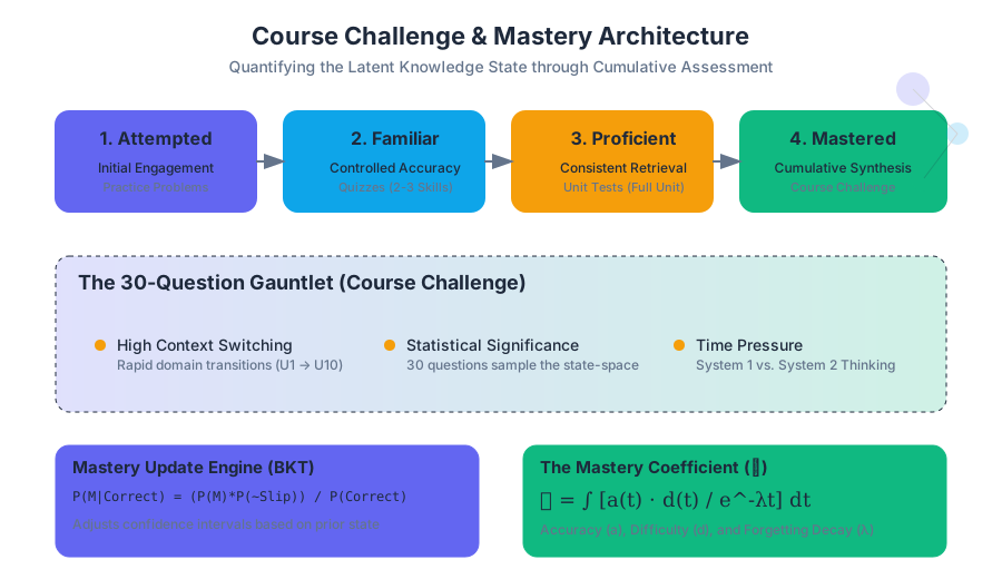
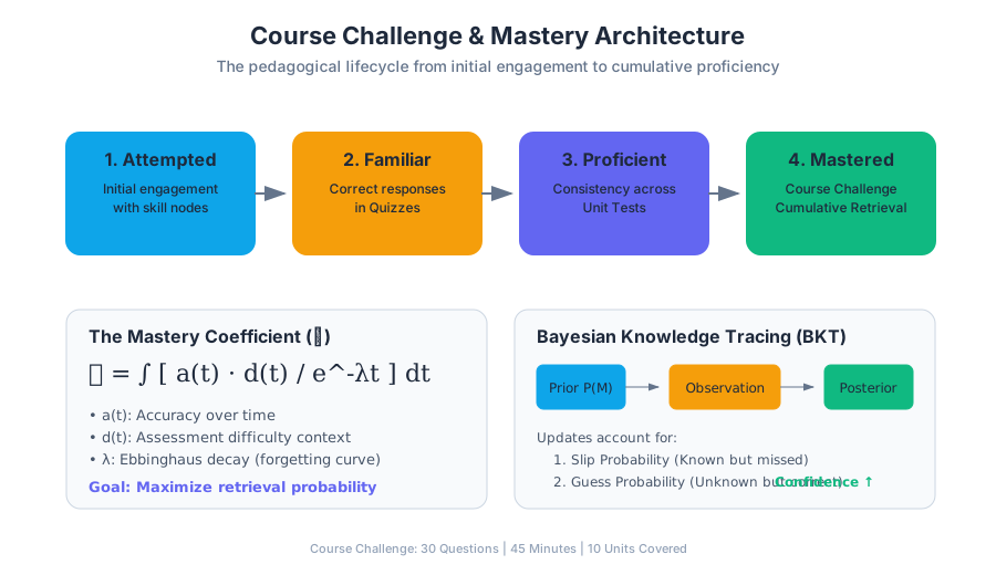
Source Materials
Study AP/College Calculus AB with AI — Free on Lykke
Sign up for free to generate personalized flashcards, quizzes, and study guides from this course. Chat with an AI tutor that knows the material.
Get Started FreeView this course wiki on Lykke · Browse all public course wikis