AP Physics 1
Institution: MIT
51 study materials · 47 sections
AP Physics 1 students working the current College Board Course and Exam Description, including first-time students with no prior background, plus teachers reviewing the page for CED alignment.; Teach every official CED unit and every numbered topic at topic granularity.; Develop every AP skill / science-practice code explicitly and by name.; Replace description with teaching: worked contextual examples, named misconceptions, and in-flow retrieval checks.; Build an exam-practice unit covering every task type on the current exam.
Course Sections
Course Framework, Skills and Reasoning Processes
Key concepts: AP Physics 1 course framework · Science practices and reasoning processes · Explaining relationships between physical quantities · Applying and justifying mathematical routines · Designing experiments and analyzing data · Making connections across course topics · Qualitative graph sketching · Selecting a logical computational pathway · Using functional dependence between variables · Supporting claims with evidence or reasoning
Physics becomes powerful when a moving object is more than a number in an equation: it becomes a physical system that can be represented, measured, modeled, tested, and explained.
Course Framework, Skills and Reasoning Processes
Physics becomes powerful when a moving object is more than a number in an equation: it becomes a physical system that can be represented, measured, modeled, tested, and explained. How can a physicist move from an observation—such as a cart speeding up—to a defensible claim about why its motion changes?
The AP Physics 1 course framework specifies what students must know, what they must be able to do, and what they must understand about foundational classical mechanics. Its central habits are explaining relationships, applying and justifying mathematical routines, designing experiments, analyzing data, and connecting ideas across multiple topics.
A course built around reasoning
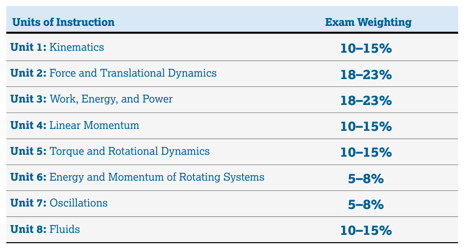
The content progresses through physical ideas that repeatedly interact:
- Kinematics describes motion.
- Force and Translational Dynamics explains changes in motion.
- Work, Energy, and Power and Linear Momentum provide conservation-based ways to analyze interactions.
- Torque and Rotational Dynamics extends force reasoning to rotation.
- Energy and Momentum of Rotating Systems connects rotational motion to conservation laws.
- Oscillations studies repeating motion.
- Fluids applies force, pressure, and conservation ideas to continuous matter.
The same science practices spiral through every topic. A problem about a satellite, a collision, a rotating wheel, or flowing water may require the same sequence: represent the situation, identify relationships, calculate or compare quantities, and support a claim with evidence or physical principles.
Science Practice 1: Creating Representations
Science Practice 1: Creating Representations means turning a physical situation into a useful diagram, table, chart, schematic, or graph. A representation is not decoration; it is a model that makes relevant relationships visible.
- 1.A. Create diagrams, tables, charts, or schematics to represent physical situations. Examples include free-body diagrams, system sketches, motion maps, circuit-like schematics for conceptual models, and data tables.
- 1.B. Create quantitative graphs with appropriate scales and units, including plotting data. A graph must identify variables, units, scale, and the measured or calculated relationship.
- 1.C. Create qualitative sketches of graphs that represent features of a model or the behavior of a physical system. A qualitative graph shows trends—such as increasing, decreasing, constant, or changing slope—even when no numerical data are supplied.
For example, if the net force on a cart increases while its mass remains constant, a qualitative sketch of acceleration versus force should rise proportionally. The sketch communicates the model before any numerical calculation begins.
Science Practice 2: Mathematical Routines
Science Practice 2: Mathematical Routines means conducting analyses to derive, calculate, estimate, or predict. The goal is not merely obtaining an answer; it is selecting a logical pathway that preserves the physical meaning of the quantities.
- 2.A. Derive a symbolic expression from known quantities by selecting and following a logical mathematical pathway. Begin with a physical law, substitute relationships, and simplify until the desired quantity is isolated.
- 2.B. Calculate or estimate an unknown quantity with units from known quantities, by selecting and following a logical computational pathway. Units act as a built-in error check.
- 2.C. Compare physical quantities between two or more scenarios or at different times and locations in a single scenario. Comparisons often require ratios rather than complete calculations.
- 2.D. Predict new values or factors of change of physical quantities using functional dependence between variables. If $F = ma$, then for fixed $m$, doubling $F$ doubles $a$; this is a prediction from functional dependence.
Worked example: A constant net force acts on two carts. Cart $A$ has mass $m$ and cart $B$ has mass $2m$. From Newton’s second law,
$$ a=\frac{F_{\text{net}}}{m}. $$
For cart $B$,
$$ a_B=\frac{F_{\text{net}}}{2m}=\frac{1}{2}a_A. $$
No numerical values are needed: 2.C compares the accelerations, while 2.D predicts the factor of change from the functional dependence.
Science Practice 3: Scientific Questioning and Argumentation
Science Practice 3: Scientific Questioning and Argumentation means describing experimental procedures, analyzing data, and supporting claims. Physics knowledge becomes stronger when a model survives measurement and criticism.
- 3.A. Create experimental procedures that are appropriate for a given scientific question. A valid procedure identifies what is changed, what is measured, what is controlled, and how repeated measurements or improved design can reduce uncertainty.
- 3.B. Apply an appropriate law, definition, theoretical relationship, or model to make a claim. For example, use conservation of momentum to claim that the total momentum of an isolated system remains constant.
- 3.C. Justify or support a claim using evidence from experimental data, physical representations, or physical principles or laws. A justification must connect evidence to the claim rather than simply repeat the result.
A strong experimental argument has the structure: claim → evidence → physical reasoning. If measured acceleration increases linearly with applied force, the data support a claim consistent with $F_{\text{net}}=ma$—provided the graph, units, uncertainty, and controlled variables are also considered.
How these skills appear in assessment
Multiple-choice questions commonly test representation interpretation, mathematical reasoning, comparisons, functional dependence, and qualitative-to-quantitative translation. Free-response questions make the reasoning visible through diagrams, symbolic derivations, calculations, experimental design, data analysis, and evidence-based explanations.
The listed weighting guidance emphasizes the importance of these practices: Creating Representations accounts for approximately $20%$–$35%$ of the free-response section; Mathematical Routines accounts for approximately $15%$–$20%$ of the multiple-choice section and $30%$–$40%$ of the free-response section. The exact task may change, but the underlying reasoning remains central.
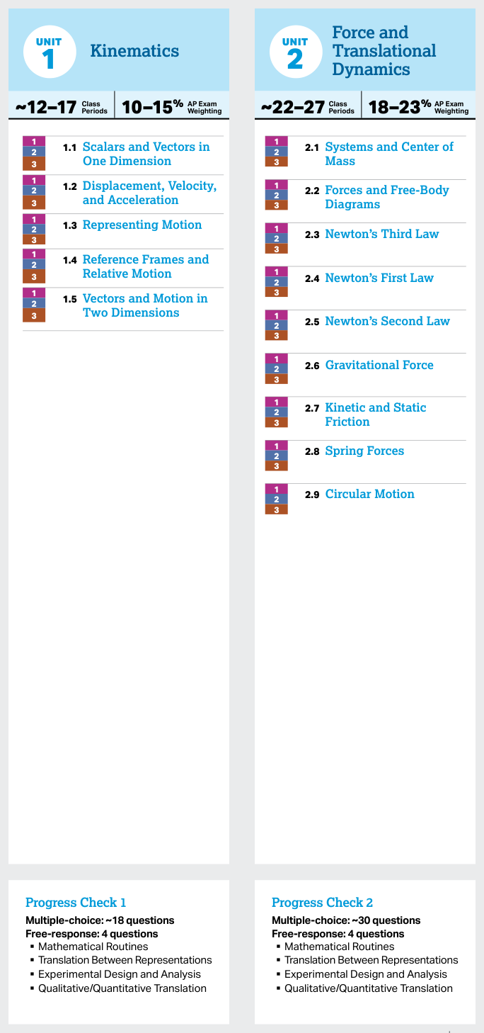
AP Classroom Progress Checks include multiple-choice questions with rationales and free-response questions with scoring information. Reports allow teachers to review results, locate patterns of difficulty, and identify where students struggle—for example, interpreting a graph, choosing a system, or justifying an experimental conclusion.
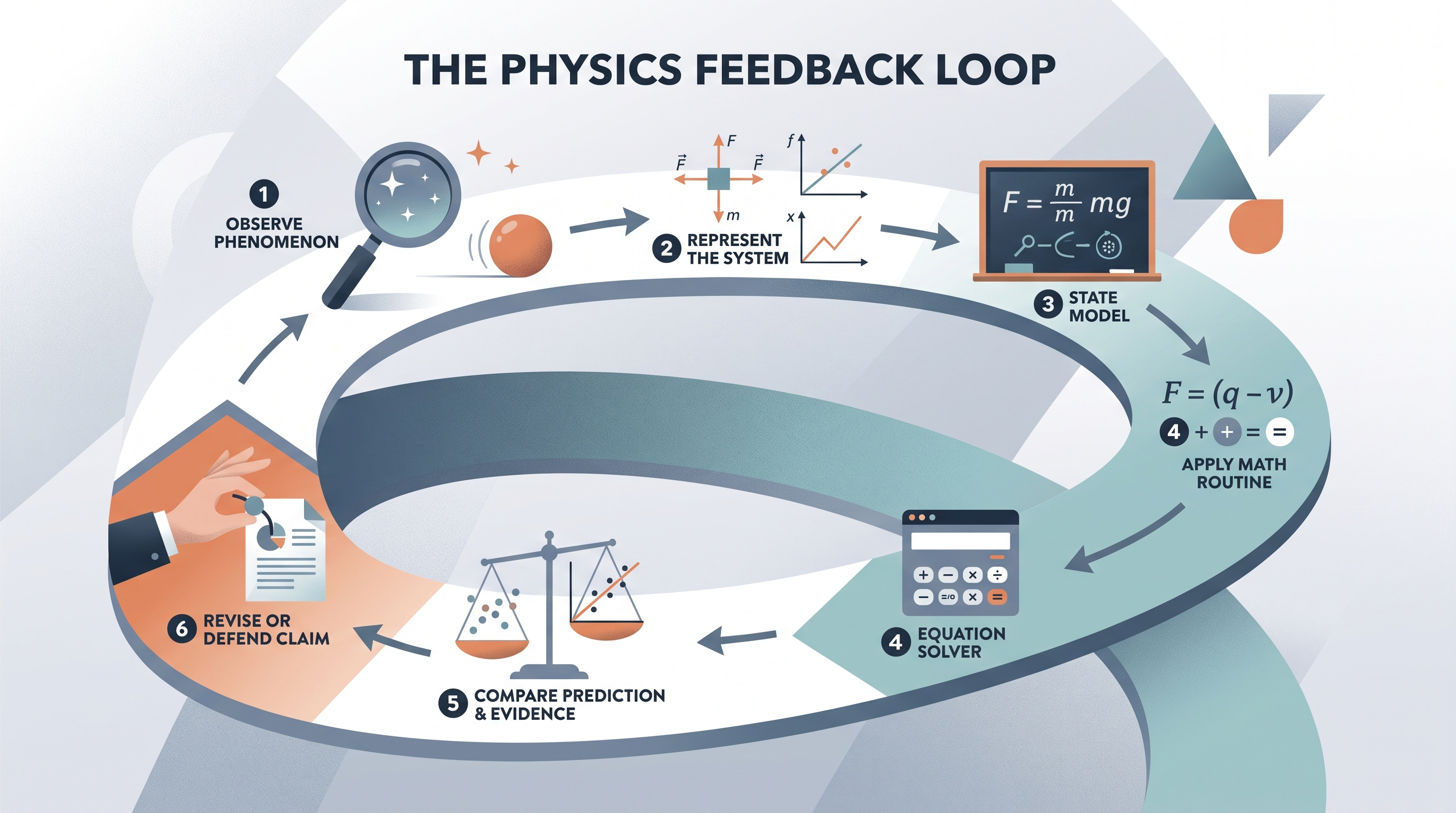
The feedback loop
Physics instruction works best as a continuous loop:
- Observe a phenomenon.
- Represent the system.
- State a relationship or model.
- Apply a mathematical routine.
- Compare the prediction with evidence.
- Revise or defend the claim.
Continuous checks of understanding and just-in-time feedback interrupt errors before they become habits. A student who writes an equation correctly but chooses the wrong system, graph, or sign convention needs conceptual feedback—not merely a corrected numerical answer.
Retrieval check: A graph’s slope changes while its measured variables remain the same. Which practice is most directly involved in interpreting that feature? A complete response should identify 1.C, then connect the changing slope to the physical model and, if appropriate, use 2.D to predict how another quantity changes.



1.1 Scalars and Vectors in One Dimension
Key concepts: Scalars and vectors in one dimension · Physical quantities · Comparing physical quantities between scenarios or at different times and locations · Representing physical situations with diagrams, tables, charts, or schematics · Applying an appropriate law, definition, or theoretical relation · Science Practice 1 · Science Practice 2 · Science Practice 3
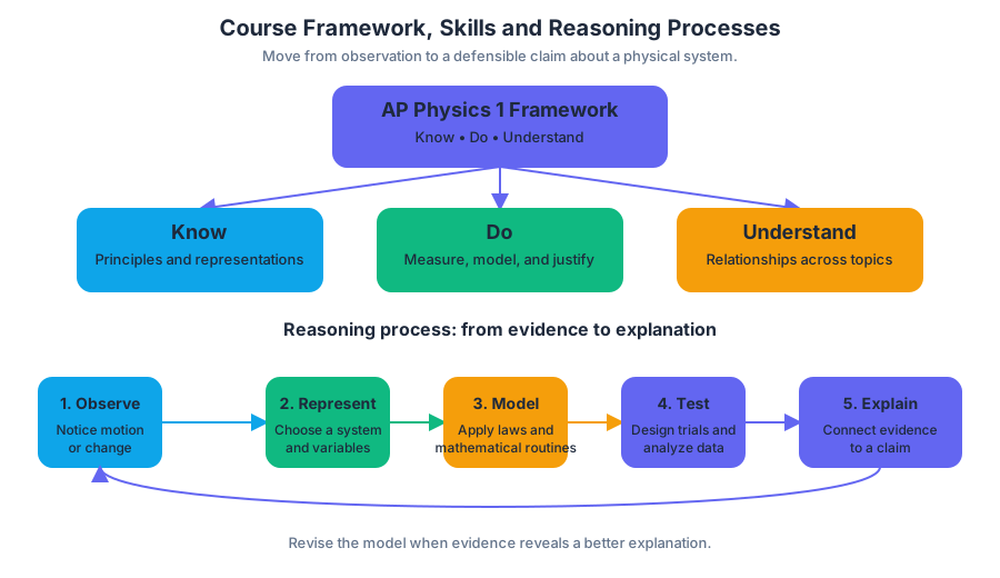
A scalar tells you how much of a physical quantity exists, while a vector tells you both how much and in which direction. A car traveling at $20\ \text{m/s}$ and a car traveling at $20\ \text{m/s}$ in the opposite direction have the same speed but different velocities because velocity includes direction.
1.1 Scalars and Vectors in One Dimension
A scalar tells you how much of a physical quantity exists, while a vector tells you both how much and in which direction. A car traveling at $20\ \text{m/s}$ and a car traveling at $20\ \text{m/s}$ in the opposite direction have the same speed but different velocities because velocity includes direction.
In one dimension, direction can be represented with a sign. Choose one direction as positive—often rightward or upward—and represent the opposite direction as negative. The sign is not an extra physical quantity; it records the vector’s direction relative to the chosen coordinate axis.
Physical quantities: amount versus direction
A physical quantity is a measurable property described by a number and a unit. Some physical quantities are scalars; others are vectors.
| Quantity | Type | Example |
|---|---|---|
| Time | Scalar | $t=4.0\ \text{s}$ |
| Mass | Scalar | $m=2.0\ \text{kg}$ |
| Distance | Scalar | $d=15\ \text{m}$ |
| Speed | Scalar | $v=6.0\ \text{m/s}$ |
| Position in one dimension | Vector-like directed quantity | $x=-3.0\ \text{m}$ |
| Displacement | Vector | $\Delta x=+8.0\ \text{m}$ |
| Velocity | Vector | $v=-5.0\ \text{m/s}$ |
| Acceleration | Vector | $a=+2.0\ \text{m/s}^2$ |
The word vector becomes especially manageable in one dimension because there are only two possible directions along an axis. In two or three dimensions, a vector requires components or an angle; here, a signed number is enough to distinguish opposite directions.
Representing a physical situation
A physical situation becomes easier to reason about when its verbal description is translated into a representation: a diagram, table, chart, or schematic. The representation should make the chosen direction, relevant locations, and measured quantities visible rather than leaving them hidden in prose.
Example: two runners on a straight path. Let east be positive. Runner A is $12\ \text{m}$ east of the starting line, and Runner B is $7\ \text{m}$ west of it.
$$ x_A=+12\ \text{m} $$
$$ x_B=-7\ \text{m} $$
A number-line representation is therefore more informative than two unsigned distances:
$$ \text{west}\qquad\leftarrow\qquad -7\ \text{m}\quad\vert\quad 0\quad\vert\quad +12\ \text{m}\qquad\rightarrow\qquad\text{east} $$
The diagram shows immediately that Runner A is farther east, while Runner B is farther west. It also prevents a common error: treating “$7\ \text{m}$ west” as merely $7\ \text{m}$ and losing the directional information.
Comparing quantities across scenarios
Skill 2.C — Compare physical quantities between two or more scenarios or at different times and locations in a single scenario. Comparison requires identifying both the numerical magnitude and, when applicable, the direction.
Suppose a robot’s position changes from $x_1=-2.0\ \text{m}$ to $x_2=+5.0\ \text{m}$. Its final position has greater magnitude than its initial position:
$$ |x_2|=5.0\ \text{m}>|x_1|=2.0\ \text{m} $$
The robot is also on the opposite side of the origin at the second time. Saying only that “$5.0$ is greater than $2.0$” is incomplete unless the comparison concerns magnitudes. For directed quantities, $+5.0\ \text{m}$ and $-2.0\ \text{m}$ are not simply “larger” and “smaller” versions of the same physical situation; they describe different directions.
Key distinction: A scalar comparison usually concerns magnitude. A vector comparison may require magnitude and direction.
Applying definitions and relationships
Skill 3.B — Apply an appropriate law, definition, theoretical relationship, or model to make a claim. A definition is not just a formula to substitute into; it tells you what physical meaning a calculation represents.
For positions measured along one axis, the displacement definition is
$$ \Delta x=x_f-x_i. $$
For the robot above,
$$ \Delta x=(+5.0\ \text{m})-(-2.0\ \text{m})=+7.0\ \text{m}. $$
The positive result means the robot’s position changed $7.0\ \text{m}$ in the positive direction. This is different from the total distance traveled if the robot changed direction along the way; that distinction becomes important when motion quantities are developed in Topic 1.2.
Science Practice 1: Creating Representations
The course framework uses numbered, color-coded science practices to identify the reasoning emphasized in each lesson. Topics $1.1$ through $1.5$ incorporate Science Practice 1: Creating Representations, Science Practice 2: Mathematical Routines, and Science Practice 3: Scientific Questioning and Argumentation. In this topic, the most direct application is Skill 1.A — Create diagrams, tables, charts, or schematics to represent physical situations.
A strong representation is selective: it includes the coordinate direction, origin, object locations, signs, and units, but does not bury the central relationship under irrelevant decoration. A useful workflow is:
- Choose and label the positive direction.
- Mark the origin or reference location.
- Assign signs to directed quantities.
- Record numerical values with units.
- Use the representation to compare or calculate.
Misconception check
Misconception: “A negative vector means the quantity is less than zero physically.” Negative position, velocity, or displacement does not mean that the object has a negative amount of motion or a negative length. It means the vector points opposite the selected positive direction.
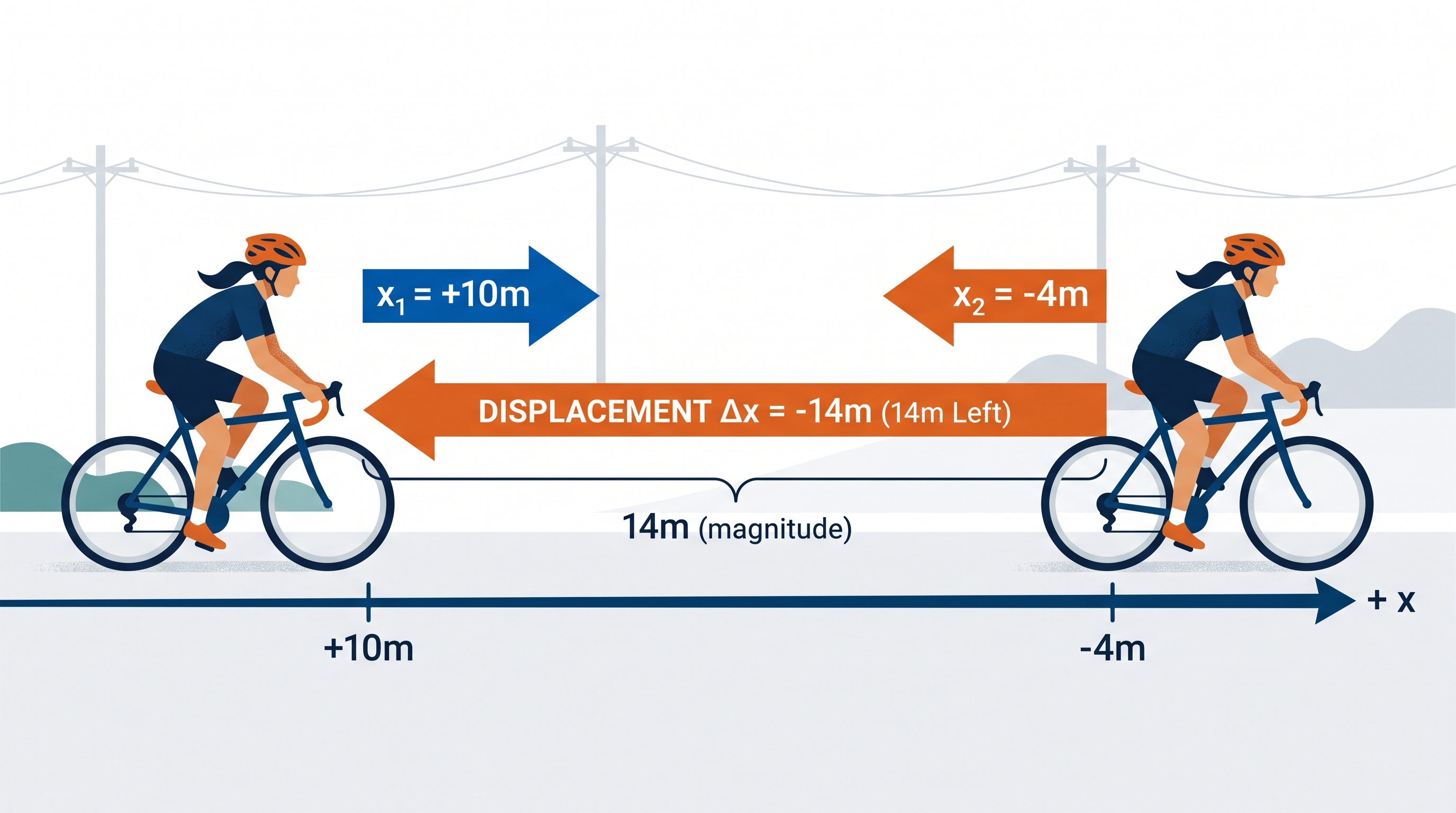
Retrieval check: A cyclist is at $x=+10\ \text{m}$ and later at $x=-4\ \text{m}$. Which position has greater magnitude, and what is the cyclist’s displacement?
The position at $x=+10\ \text{m}$ has greater magnitude because $|+10|>|-4|$. The displacement is
$$ \Delta x=(-4\ \text{m})-(+10\ \text{m})=-14\ \text{m}, $$
so the cyclist moved $14\ \text{m}$ in the negative direction.


1.2 Displacement, Velocity, and Acceleration
Key concepts: Displacement, velocity, and acceleration in one-dimensional motion · Qualitative sketches of graphs representing physical-system behavior · Comparing physical quantities across scenarios, times, or locations · Calculating or estimating unknown quantities with units · Vectors represented visually as arrows with direction and length proportional to magnitude · Average velocity · Average acceleration · Constant-acceleration kinematic relationships · Simple harmonic motion displacement, velocity, and acceleration · Extrema and zeros of displacement, velocity, and acceleration in harmonic motion
Over a trip, an object can have zero net displacement even while having nonzero velocity and acceleration during parts of the trip.
1.2 Displacement, Velocity, and Acceleration
Over a trip, an object can have zero net displacement even while having nonzero velocity and acceleration during parts of the trip.
A runner who leaves a starting line, travels $50\ \text{m}$ east, and returns to the starting line has displacement $\Delta x = 0$, but the runner’s velocity is nonzero while moving and acceleration is generally nonzero while speeding up, slowing down, or reversing direction.
Displacement: the interval-to-interval change in position
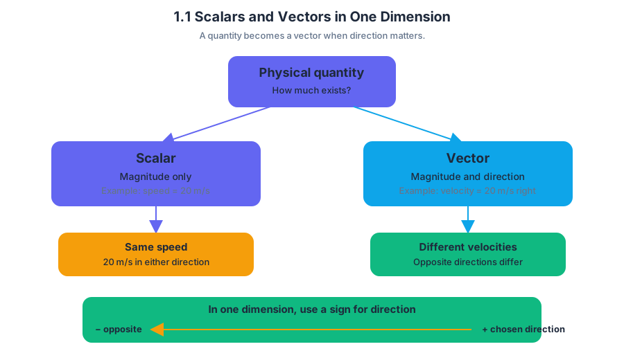
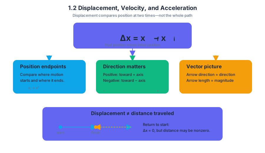
Displacement is the change in position over a time interval:
$$ \Delta x = x_f-x_i $$
The sign records direction along the chosen one-dimensional axis. A positive displacement means the final position lies in the positive direction from the initial position; a negative displacement means it lies in the negative direction. Displacement is not the same as total distance traveled: distance counts the entire path, while displacement compares only the beginning and ending positions.
Key distinction: Returning to the starting position makes displacement zero, not necessarily distance, velocity, or acceleration zero.
A vector can be represented visually by an arrow: its direction shows the vector’s direction, and its length is proportional to its magnitude. Thus, a displacement arrow pointing east and twice as long as another represents twice the displacement magnitude in the same direction.
Average velocity and average acceleration
Average velocity is displacement divided by the elapsed time:
$$ v_{\text{avg}}=\frac{\Delta x}{\Delta t} $$
Because displacement is directional, average velocity is directional as well. Average acceleration is the change in velocity divided by the time interval:
$$ a_{\text{avg}}=\frac{\Delta v}{\Delta t} $$
Acceleration describes how velocity changes, not merely whether an object is moving. An object can accelerate while its speed decreases, such as when a car moving east brakes and its acceleration points west.
Worked example — braking bicycle. A bicycle travels east at $12\ \text{m/s}$ and slows to $4\ \text{m/s}$ in $2.0\ \text{s}$. Taking east as positive,
$$ a_{\text{avg}}=\frac{v_f-v_i}{\Delta t} =\frac{4\ \text{m/s}-12\ \text{m/s}}{2.0\ \text{s}} =-4.0\ \text{m/s}^2 $$
The negative sign means the acceleration points west. The bicycle still has positive velocity, so it continues east while slowing.
Named misconception — “negative acceleration means slowing down.” Not always. An object slows down when acceleration and velocity point in opposite directions. If both are negative, the object moves in the negative direction and speeds up.
Constant-acceleration relationships
When acceleration is constant in one dimension, three equations connect velocity, time, position, and displacement:
$$ v_x=v_{x0}+a_xt $$
$$ x=x_0+v_{x0}t+\frac{1}{2}a_xt^2 $$
$$ v_x^2=v_{x0}^2+2a_x(x-x_0) $$
Here, $x_0$ and $v_{x0}$ are the initial position and velocity, while $x$ and $v_x$ are the position and velocity at time $t$. Choose the equation whose known quantities match the problem; do not use the third equation when time is essential to the requested result.
Worked example — dropped package. A package is released from rest and falls for $3.0\ \text{s}$ near Earth. Let upward be positive, so $v_{x0}=0$ and $a_x=-9.8\ \text{m/s}^2$.
Final velocity:
$$ v_x=0+(-9.8\ \text{m/s}^2)(3.0\ \text{s}) =-29.4\ \text{m/s} $$
Displacement:
$$ x-x_0=0+\frac{1}{2}(-9.8\ \text{m/s}^2)(3.0\ \text{s})^2 =-44.1\ \text{m} $$
The package is $44.1\ \text{m}$ below its release point and is moving downward at $29.4\ \text{m/s}$.
Qualitative motion and harmonic motion
A qualitative sketch should show physically meaningful features: whether position is increasing or decreasing, whether velocity is positive or negative, and whether acceleration points in the positive or negative direction. In simple harmonic motion, such as a mass attached to an ideal spring, these quantities repeatedly reach maxima, minima, and zeros.
At maximum positive displacement, the object momentarily stops, so velocity is zero; acceleration points toward equilibrium and has large negative magnitude. At equilibrium, displacement is zero and speed is greatest; acceleration is zero. At maximum negative displacement, velocity is again zero, while acceleration points back toward equilibrium in the positive direction.
This pattern exposes another misconception: zero velocity does not imply zero acceleration. At a turning point, velocity is instantaneously zero, but the acceleration is what reverses the motion.
AP skills in action
Topic 1.2 Displacement, Velocity, and Acceleration explicitly develops 1.C: Create qualitative sketches of graphs that represent features of a model or the behavior of a physical system; 2.B: Calculate or estimate an unknown quantity with units from known quantities, by selecting and following a logical computational pathway; 2.C: Compare physical quantities between two or more scenarios or at different times and locations in a single scenario; 3.B: Apply an appropriate law, definition, theoretical relationship, or model to make a claim; and 3.C: Justify or support a claim using evidence from experimental data, physical representations, or physical principles or laws.
Retrieval check: A cart moves from $x=2\ \text{m}$ to $x=-6\ \text{m}$ in $4\ \text{s}$. What are its displacement and average velocity? If its velocity changes from $-3\ \text{m/s}$ to $5\ \text{m/s}$ during that interval, what is its average acceleration?
Answer: $\Delta x=-8\ \text{m}$, $v_{\text{avg}}=-2\ \text{m/s}$, and $a_{\text{avg}}=2\ \text{m/s}^2$. The cart’s displacement and average velocity are negative, but its average acceleration is positive because its velocity increased by $8\ \text{m/s}$.
1.3 Representing Motion
Key concepts: Representing physical situations with diagrams, tables, charts, and schematics · Creating qualitative sketches of graphs to show features of a model or behavior · Applying physical laws, definitions, theoretical relationships, and models to make claims · Simple harmonic motion of a mass-spring oscillator · Energy bar charts for a spring oscillator · Rolling without slipping · Rotational inertia of a uniform disk · Inelastic collision of a falling block with a moving cart · Pulley systems with a lightweight string · Interpreting motion through experimental setups and labeled force diagrams
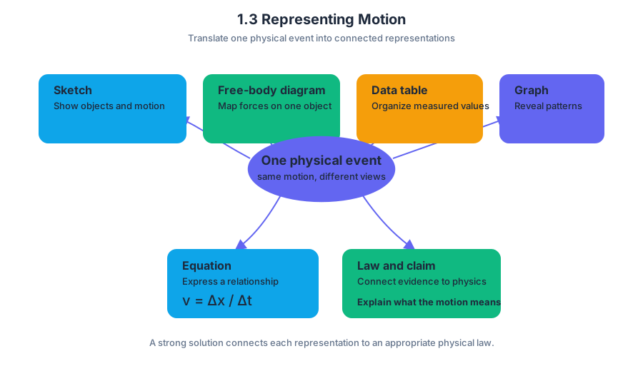
A motion problem becomes much easier when the physical situation is translated into several representations: a sketch of the objects, a free-body diagram, a data table, a graph, and an equation.
1.3 Representing Motion
A motion problem becomes much easier when the physical situation is translated into several representations: a sketch of the objects, a free-body diagram, a data table, a graph, and an equation. Each representation highlights a different feature of the same event.
Learning Objective 1.3.A: Represent the motion of an object using diagrams, graphs, charts, and mathematical representations.
The essential knowledge for this topic is commonly identified through the idea that physical situations can be represented in multiple forms. A strong solution does not merely draw or calculate; it connects the representation to an appropriate physical law and uses that law to support a claim.
From physical scene to physical model
Begin with a system sketch: identify the relevant objects, the surface or environment, the direction of motion, and important dimensions or angles. Then construct a free-body diagram, which shows only the chosen object and the external forces acting on it. The diagram should make directions explicit rather than relying on the reader to infer them.
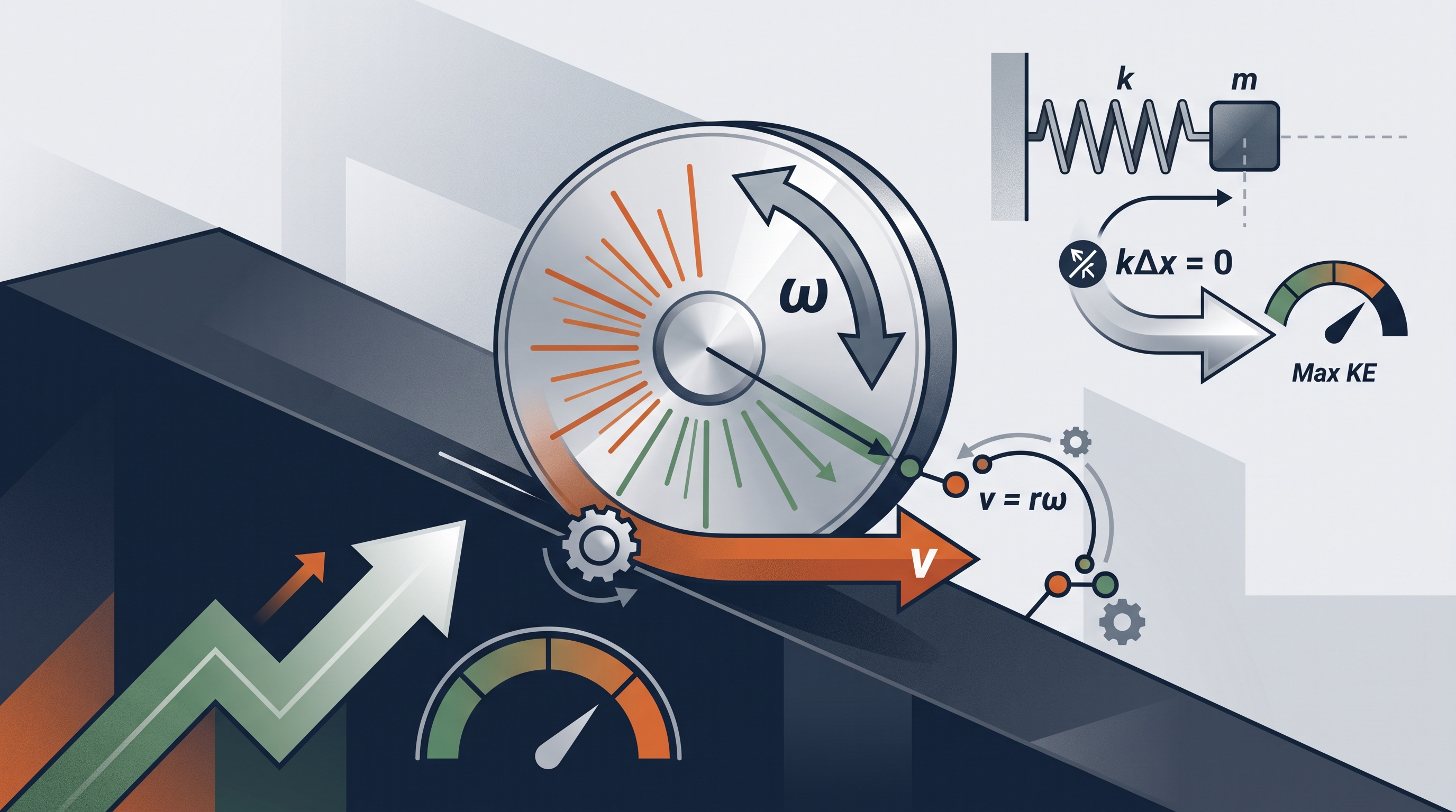
For example, a disk rolls down an incline without slipping. Its rotational inertia is
$$ I_{\text{disk}}=\frac{1}{2}MR^2. $$
A useful representation includes the disk, the incline angle $\theta$, the radius $R$, the mass $M$, the direction down the ramp, the normal force, the gravitational force, and static friction $F_f$. The phrase without slipping is not decorative: it supplies the model relationship
$$ v=R\omega, $$
where $v$ is the center-of-mass speed and $\omega$ is the angular speed. Applying this relationship supports the claim that the disk has both translational and rotational motion.
Qualitative graphs show behavior
A qualitative graph shows important features—such as increasing, decreasing, constant, maximum, minimum, or changing slope—without requiring exact numerical values. For a spring oscillator, position varies periodically, velocity is greatest near equilibrium, and acceleration points toward equilibrium.
A horizontal mass-spring system consists of a mass $m$ attached to a wall by a spring. If the mass is displaced to $x=-x_0$ and released, the spring pulls it toward the equilibrium position $x=0$. The motion is simple harmonic motion, a special type of periodic motion in which the restoring force is proportional to displacement and directed toward equilibrium:
$$ F_x=-kx. $$
The minus sign is essential. If $x$ is positive, the force is negative; if $x$ is negative, the force is positive. A graph of $F_x$ versus $x$ is therefore a straight line through the origin with slope $-k$.
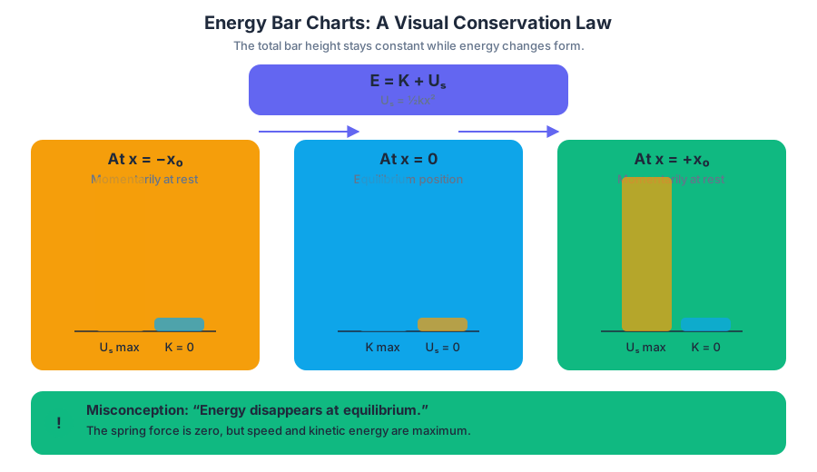
Energy bar charts: a visual conservation law
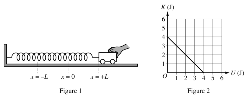
An energy bar chart represents how the system’s energy is distributed at selected moments. For an ideal spring oscillator, the total mechanical energy remains constant:
$$ E=K+U_s, \qquad U_s=\frac{1}{2}kx^2. $$
At $x=-x_0$, the mass is momentarily at rest, so the chart contains maximum spring potential energy and zero kinetic energy. At $x=0$, the spring potential energy is zero relative to that equilibrium reference, and kinetic energy is maximum. The total height of the bars must remain unchanged unless energy enters or leaves the chosen system.
Misconception check — “The energy disappears at equilibrium.” At equilibrium, the spring force is zero, but the mass is moving fastest. Energy has changed form from spring potential energy to kinetic energy; it has not vanished.
Linking representations in a collision
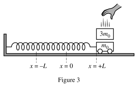
Suppose a cart moves horizontally at constant speed and a block is dropped vertically onto it from rest. The block sticks to the cart. A before-and-after sketch should show the cart’s initial horizontal velocity, the block’s zero initial horizontal velocity, and the shared final velocity.
Because there is no horizontal sliding after impact, the cart and block move together horizontally. For the cart-block system, horizontal momentum is conserved if the external horizontal impulse is negligible:
$$ m_c v_{c,i}+m_b v_{b,i}
(m_c+m_b)v_f. $$
Since the block is dropped from rest, $v_{b,i}=0$, giving
$$ v_f=\frac{m_c v_{c,i}}{m_c+m_b}. $$
Misconception check — “Sticking collisions conserve kinetic energy.” They generally do not. Momentum can be conserved while kinetic energy decreases because energy is transferred to deformation, sound, and thermal energy.
A pulley representation
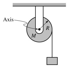
A lightweight string wrapped around a pulley and connected to a hanging block provides another translation between representations. The block’s downward displacement corresponds to the pulley’s angular displacement. If the string remains taut and does not slip,
$$ v=R\omega, \qquad a=R\alpha. $$
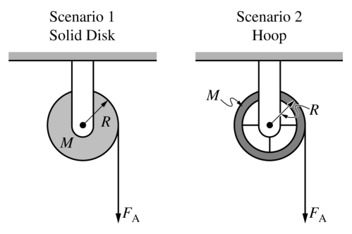
A complete diagram identifies the block, pulley, string, directions of motion, tension, gravity, and axle forces. The correct rotational model then connects torque and angular acceleration rather than treating the pulley as a point mass.
AP skills used in this topic
The principal science practices are:
- 1.A — Create diagrams, tables, charts, or schematics to represent physical situations.
- 1.C — Create qualitative sketches of graphs that represent features of a model or the behavior of a physical system.
- 2.A — Derive a symbolic expression from known quantities by selecting and following a logical mathematical pathway.
- 2.B — Calculate or estimate an unknown quantity with units using a logical computational pathway.
- 2.D — Predict new values or factors of change of physical quantities using functional dependence between variables.
- 3.B — Apply an appropriate law, definition, theoretical relationship, or model to make a claim.
- 3.C — Justify or support a claim using evidence from experimental data, physical representations, or physical principles or laws.
Retrieval check
A disk rolls down an incline without slipping. Which representation must show rotational inertia, and which relationship connects its linear and angular motion? Why can a spring oscillator have zero spring force while possessing maximum kinetic energy?
1.4 Reference Frames and Relative Motion
Key concepts: Reference frames · Relative motion · Motion described relative to a reference frame · Measurements from a given reference frame · Relationships between objects in a single scenario · One-dimensional relative motion · Accelerating (non-inertial) reference frames · Models and representations of physical systems · Qualitative sketches of graphs · Applying laws, definitions, theoretical relationships, or models to make claims
A passenger sitting on a moving train is at rest relative to the train but moving relative to the ground. Both descriptions are correct because motion is measured relative to a reference frame—the coordinate system and observer chosen to describe position and time.
1.4 Reference Frames and Relative Motion
A passenger sitting on a moving train is at rest relative to the train but moving relative to the ground. Both descriptions are correct because motion is measured relative to a reference frame—the coordinate system and observer chosen to describe position and time.
The same motion, different observers
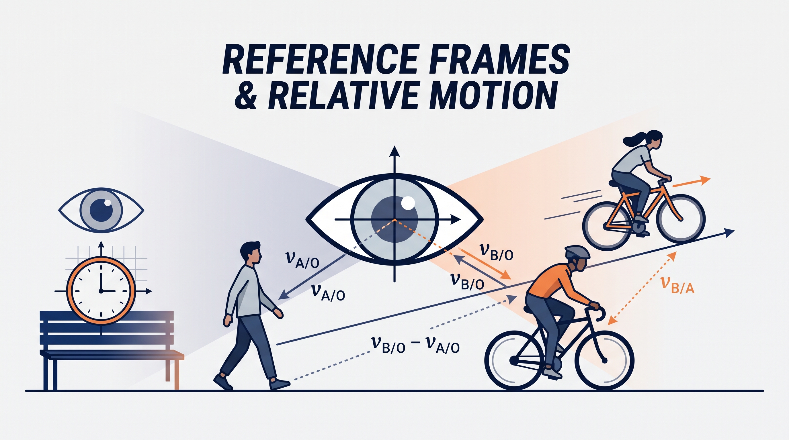
A reference frame is the viewpoint, coordinate system, and clock used to measure an object’s location and motion. Position, displacement, velocity, and acceleration are not meaningful until the reference frame is specified.
Learning Objective 1.4.A: Describe the reference frame of a given observer.
Essential Knowledge 1.4.A.1: A reference frame is a coordinate system relative to which measurements of position, distance, displacement, velocity, and acceleration are made.
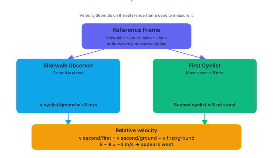
Imagine a cyclist traveling east at $8\ \text{m/s}$ past a stationary observer on the sidewalk. The sidewalk observer measures the cyclist’s velocity as
$$ v_{\text{cyclist/ground}}=+8\ \text{m/s}. $$
A second cyclist rides east at $5\ \text{m/s}$. To the first cyclist, the second cyclist moves east at only
$$ v_{\text{second/first}}=v_{\text{second/ground}}-v_{\text{first/ground}} =5-8=-3\ \text{m/s}. $$
The negative sign means that the second cyclist appears to move west relative to the first cyclist—even though both cyclists move east relative to the ground.
Relative velocity: “of” relative to “with respect to”
Relative motion describes how one object’s position changes as measured from another object or reference frame. The notation makes the viewpoint explicit:
$$ v_{A/B}=\text{velocity of object }A\text{ relative to reference frame }B. $$
For one-dimensional motion, relative velocities combine algebraically:
$$ v_{A/C}=v_{A/B}+v_{B/C}. $$
Equivalently, if both velocities are measured relative to the ground,
$$ v_{A/B}=v_{A/\text{ground}}-v_{B/\text{ground}}. $$
The subtraction is not an extra physical force or interaction. It is a comparison of two measurements made along the same axis. Choose a positive direction first, then attach signs to every velocity.
Worked example: two trains
Train $A$ travels east at $20\ \text{m/s}$, while train $B$ travels west at $12\ \text{m/s}$. Let east be positive:
$$ v_{A/\text{ground}}=+20\ \text{m/s}, \qquad v_{B/\text{ground}}=-12\ \text{m/s}. $$
The velocity of train $A$ relative to train $B$ is
$$ v_{A/B}=20-(-12)=+32\ \text{m/s}. $$
Thus, train $A$ approaches train $B$ at $32\ \text{m/s}$. Their relative separation decreases at that rate.
Misconception check — “opposite directions require adding automatically.”
Velocities are always added or subtracted according to the signed equation. Here, subtraction of a negative velocity produces addition. The signs—not a memorized direction rule—determine the result.
Locations and relationships in one scenario
A useful representation shows every object, its location, its direction, and the chosen reference frame. For objects on a straight track, a number line is often enough.
Suppose a dog is at position $x_D=14\ \text{m}$ and a runner is at position $x_R=6\ \text{m}$. The dog’s position relative to the runner is
$$ x_{D/R}=x_D-x_R=14-6=8\ \text{m}. $$
If the dog runs at $+4\ \text{m/s}$ and the runner at $+2\ \text{m/s}$, then
$$ v_{D/R}=4-2=+2\ \text{m/s}. $$
The dog is $8\ \text{m}$ ahead and is moving farther ahead at $2\ \text{m/s}$. If both move at $4\ \text{m/s}$, then $v_{D/R}=0$, so the dog remains stationary relative to the runner even though both move relative to the ground.
Inertial reference frames
An inertial reference frame is one moving at constant velocity relative to another inertial frame. In the AP Physics 1 model, observers in different inertial frames can disagree about position and velocity, but ordinary Newtonian relationships remain consistent.
Students are not expected to account for accelerating, or non-inertial, reference frames unless a problem explicitly mentions them. If a bus accelerates while you stand inside it, the bus frame is non-inertial; do not introduce that complication unless the prompt requires it.
Graphs as reference-frame evidence
A position–time graph changes when the reference frame changes. If two objects have identical constant velocities relative to the ground, their separation remains constant, so a graph of relative position versus time is horizontal:
$$ x_{A/B}(t)=\text{constant}. $$
If $v_{A/B}$ is constant but nonzero, the relative-position graph is a straight line whose slope is $v_{A/B}$. A positive slope means the separation coordinate increases; a negative slope means it decreases.
Retrieval check: A skateboard moves east at $6\ \text{m/s}$ beside a cyclist moving east at $6\ \text{m/s}$. What does the cyclist measure for the skateboard’s velocity?
Answer: $v_{\text{skateboard/cyclist}}=6-6=0\ \text{m/s}$; the skateboard is at rest in the cyclist’s frame.
AP skills assessed in Topic 1.4
Topic 1.4 explicitly develops these AP skills:
- 1.C — Create qualitative sketches of graphs that represent features of a model or the behavior of a physical system. Sketch relative position or velocity graphs from the signs and constancy of relative motion.
- 2.A — Derive a symbolic expression from known quantities by selecting and following a logical mathematical pathway. Derive $v_{A/B}=v_{A/C}-v_{B/C}$ from the relative-velocity relationship.
- 2.B — Calculate or estimate an unknown quantity with units from known quantities, by selecting and following a logical computational pathway. Substitute signed velocities and report units.
- 3.C — Justify or support a claim using evidence from experimental data, physical representations, or physical principles or laws. Use a number-line model, graph, or velocity relationship to defend a statement about what an observer measures.
The central habit is to label every measurement with its observer: relative to whom? Once that label is explicit, one-dimensional relative-motion problems become a controlled comparison of positions and velocities rather than a clash between apparently contradictory descriptions.
1.5 Vectors and Motion in Two Dimensions
Key concepts: Vectors and vector components · Motion in two dimensions · Projectile motion · Predicting a projectile’s landing spot · Quantitative graphs from data · Applying physical laws to make claims · Newton’s second law · Circular motion · Conservation of energy · Relationships between physical quantities in different scenarios
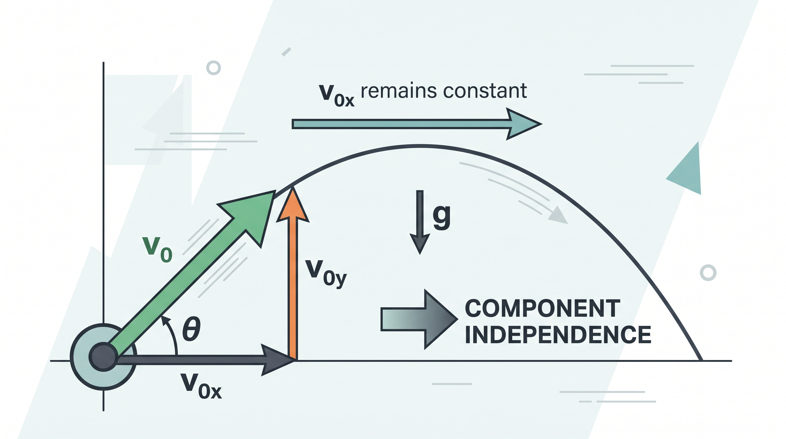
A projectile can move rightward while accelerating downward, because its motion has independent perpendicular components. Learning Objective 1.5.B: describe the motion of an object moving in two dimensions.
1.5 Vectors and Motion in Two Dimensions
A projectile can move rightward while accelerating downward, because its motion has independent perpendicular components. Learning Objective 1.5.B: describe the motion of an object moving in two dimensions.
Vectors: one motion, two perpendicular components
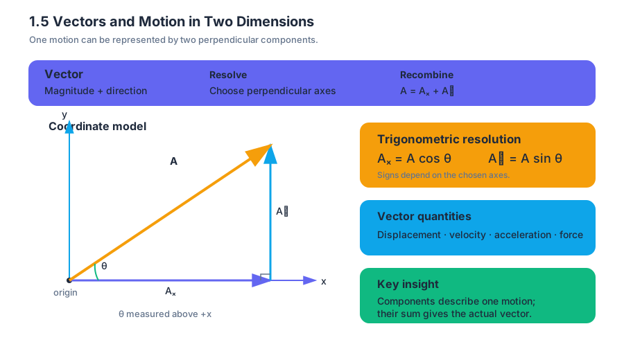
A vector is a quantity with both magnitude and direction. Displacement, velocity, acceleration, and force are vectors; time, mass, and temperature are scalars because they have magnitude but no direction. A two-dimensional vector can be modeled as the result of two perpendicular components.
For a vector $\vec{A}$ with magnitude $A$ and angle $\theta$ measured above the positive $x$-axis,
$$ A_x=A\cos\theta $$
$$ A_y=A\sin\theta $$
The signs of $A_x$ and $A_y$ depend on the chosen coordinate system. This is the essential idea behind 1.5.A.1: Vectors are modeled as the result of two perpendicular components, 1.5.A.2: Vectors are resolved into components based on a chosen coordinate system, and 1.5.A.3: Trigonometric functions are used to resolve vectors into perpendicular components.
Key insight: The components are not two separate motions replacing the original motion. They are two mathematically convenient descriptions whose vector sum gives the actual vector.
Worked example: launch velocity
A ball leaves a ramp at $12\ \text{m/s}$, directed $30^\circ$ above horizontal. Resolve its velocity into components:
$$ v_{0x}=(12)\cos 30^\circ\approx 10.4\ \text{m/s} $$
$$ v_{0y}=(12)\sin 30^\circ=6.0\ \text{m/s} $$
The ball initially moves right at $10.4\ \text{m/s}$ and upward at $6.0\ \text{m/s}$. Skill 2.A: Deriving symbolic expressions is used when these relationships are obtained from the geometry; 2.B: Calculate or estimate an unknown quantity with units from known quantities, by selecting and following a logical computational pathway is used when numerical values are calculated.
Misconception check — “the vertical velocity is the total velocity.” The vertical component is only one part of the velocity. The total speed is recovered from
$$ v=\sqrt{v_x^2+v_y^2}. $$
Projectile motion
Ignoring air resistance, a projectile has constant horizontal velocity and constant downward vertical acceleration:
$$ a_x=0,\qquad a_y=-g. $$
Therefore,
$$ x=x_0+v_{0x}t $$
and
$$ y=y_0+v_{0y}t-\frac{1}{2}gt^2. $$
The horizontal and vertical equations share the same time $t$. That shared time connects the two independent components into one two-dimensional path.
Predicting a landing spot
A projectile is launched horizontally from a platform $20\ \text{m}$ above level ground at $8.0\ \text{m/s}$. Its horizontal landing distance can be predicted without first finding its final speed.
Vertical motion determines the flight time:
$$ 20=\frac{1}{2}gt^2 $$
$$ t=\sqrt{\frac{40}{9.8}}\approx 2.02\ \text{s}. $$
Horizontal motion then gives
$$ \Delta x=v_xt=(8.0)(2.02)\approx 16.2\ \text{m}. $$
The predicted landing spot is approximately $16\ \text{m}$ from the platform’s edge. Skill 2.D: Predicting values based on functional dependencies appears here: the horizontal position depends linearly on time, while the vertical position depends quadratically on time.
Misconception check — “gravity makes the projectile move forward.” Gravity changes only the vertical component in this ideal model. The projectile continues moving horizontally because its horizontal velocity remains constant.
Graphs, data, and physical claims
A motion investigation can turn measured positions and times into a quantitative graph. For horizontal projectile motion, a graph of $x$ versus $t$ should be linear; its slope represents $v_x$. For vertical motion, a graph of $y$ versus $t^2$ is linear when the projectile starts with zero vertical velocity, with slope related to $-\frac{1}{2}g$.
Skill 1.B: Creating quantitative graphs from data requires selecting meaningful axes, labeling variables and units, plotting data, and identifying the relationship. Skill 3.C: Support claims with experimental evidence or physical principles requires more than saying “the graph looks right”: a claim should cite the pattern, slope, or relevant law.
For example, if measured horizontal positions increase by approximately equal amounts during equal time intervals, the data support the claim that $v_x$ is approximately constant. Skill 3.A: Designing experimental procedures enters when deciding how to measure time and position, how to repeat trials, and how to reduce uncertainty.
Connecting motion to force and energy
The acceleration components can be connected to forces using Newton’s second law:
$$ \sum \vec{F}=m\vec{a}. $$
For a projectile near Earth with negligible air resistance, the net force is its weight, so
$$ \sum F_y=-mg \quad\Rightarrow\quad a_y=-g. $$
This is a model-based claim: the force law explains the observed downward curvature.
Circular motion provides another important connection. At the top of a vertical loop, the minimum speed needed to maintain contact occurs when the normal force is just zero:
$$ \frac{mv^2}{r}=mg \quad\Rightarrow\quad v_{\min}=\sqrt{gr}. $$
If an object begins at height $h_i$ and must reach the top of the loop at height $h_t$ with this speed, conservation of energy gives
$$ mgh_i= mgh_t+\frac{1}{2}mv_{\min}^2. $$
Substituting $v_{\min}^2=gr$,
$$ h_i=h_t+\frac{r}{2}. $$
The mass cancels, allowing the required initial potential energy or starting height to be found by working backward from the needed speed.
Misconception check — “minimum speed means zero force.” At the top of the loop, the normal force is zero, but gravity is not. Gravity alone supplies the required centripetal acceleration.
Retrieval check
A ball is launched at angle $\theta$ with speed $v_0$. State the expressions for $v_{0x}$ and $v_{0y}$, identify which component changes during ideal projectile motion, and explain why a graph of horizontal position versus time is linear. A complete response should use the component model, Newton’s second law, and evidence from the graph rather than relying only on a numerical answer.
2.1 Systems and Center of Mass
Key concepts: Center of mass of a system · Weighted-average position of mass · Center of mass along a given axis · Modeling a system as a single object located at its center of mass · Finding the center of mass by visual inspection of symmetrical objects
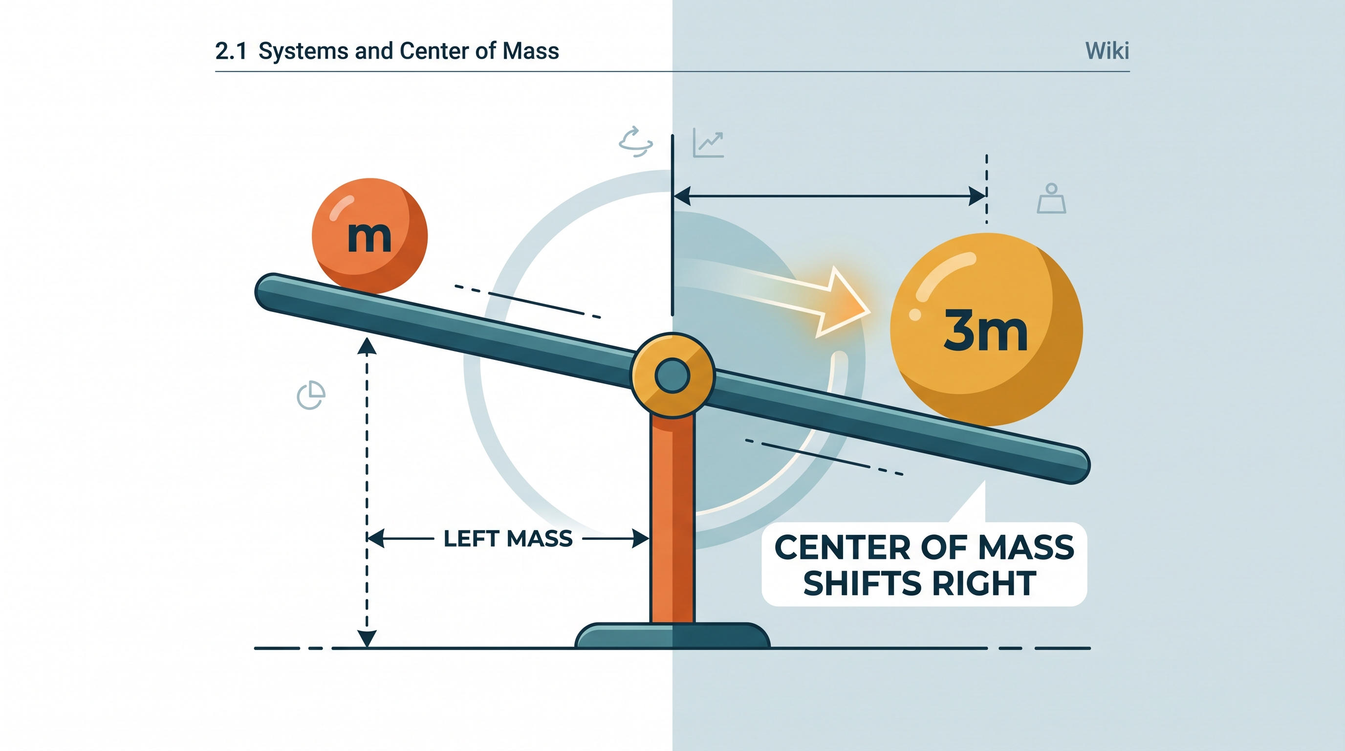
A balanced seesaw does not “care” about every particle separately; for many translational questions, it behaves as though all of its mass were concentrated at one representative location: its center of mass.
2.1 Systems and Center of Mass
A balanced seesaw does not “care” about every particle separately; for many translational questions, it behaves as though all of its mass were concentrated at one representative location: its center of mass. That location shifts toward the heavier side, even when the objects are separated and the system has no physical object at the center itself.
The center of mass as a representative location
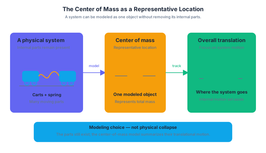
The center of mass is the representative location of a system’s mass. It is the position at which the entire system can be modeled, for certain purposes, as a single object.
Essential Knowledge 2.1.B.3: A system can be modeled as a singular object that is located at the system’s center of mass.
This is a modeling choice, not a claim that the system has physically collapsed. Two carts connected by a spring, several particles, or a lopsided object still contain internal parts. The center-of-mass model tracks the overall translational location of the system while temporarily ignoring the details of how the parts move relative to one another.
Why mass acts as a weight
The center of mass is a weighted average of the individual positions. A heavier mass contributes more strongly to the result than a lighter mass at the same distance.
For a system whose masses lie along a specified axis, the center-of-mass position is
$$ \vec{x}_{cm}=\frac{\sum m_i\vec{x}_i}{\sum m_i}. $$
Here, $m_i$ is the mass of particle $i$, $\vec{x}i$ is that particle’s position along the chosen axis, and $\vec{x}{cm}$ is the center-of-mass location along that axis. The denominator, $\sum m_i$, is the total mass of the system. The numerator adds each position after multiplying it by the mass associated with that position.
The arrows emphasize that position has direction. In a one-dimensional calculation, choose an origin and assign positive and negative coordinates. A mass to the left of the origin might have $x_i<0$, while a mass to the right has $x_i>0$.
Worked example: two unequal masses
A $2.0\ \text{kg}$ mass is at $x_1=0\ \text{m}$, and a $6.0\ \text{kg}$ mass is at $x_2=4.0\ \text{m}$. The center of mass is
$$ x_{cm}
\frac{(2.0\ \text{kg})(0\ \text{m})+(6.0\ \text{kg})(4.0\ \text{m})} {2.0\ \text{kg}+6.0\ \text{kg}}
\frac{24\ \text{kg}\cdot\text{m}}{8.0\ \text{kg}}
3.0\ \text{m}. $$
The result is $3.0\ \text{m}$ from the origin, closer to the $6.0\ \text{kg}$ mass at $4.0\ \text{m}$. That direction is physically sensible: the heavier mass pulls the weighted average toward itself.
Symmetry can reveal the answer immediately
Not every center of mass needs a calculation. For an object or arrangement with symmetrical mass, the center of mass can be found by visual inspection: it lies on the object’s symmetry line or at the intersection of its symmetry lines.
For example, the center of mass of a uniform rectangular plate is at the intersection of its diagonals. The center of mass of a uniform circular disk is at its geometric center. If equal masses are arranged symmetrically about an axis, their contributions on opposite sides balance.
Symmetry does not mean “the geometric center is always correct.” A geometric center gives the center of mass only when the mass distribution is symmetric in the relevant direction. Adding a heavy battery to one side of a robot shifts the center of mass toward the battery.
Scope and AP reasoning skills
Essential Knowledge 2.1.B.2 requires calculating the center-of-mass location along a given axis using the weighted-average equation. The AP boundary limits these calculations to systems of five or fewer particles arranged in two dimensions or to systems that are highly symmetrical; calculus-based continuous, nonuniform mass distributions are outside this expectation.
This topic develops Science Practice 1: Creating Representations, especially representing a system with a coordinate diagram and identifying symmetry. It also develops Science Practice 2: Mathematical Routines, because the solver must define an axis, assign signed positions, substitute masses and coordinates, and interpret the result physically. When a student explains why the answer must lie nearer the heavier mass, the student is using Science Practice 3: Scientific Questioning and Argumentation by supporting a claim with a physical reason.
Misconception check
Misconception: “The center of mass must be inside the material.” Not necessarily. For a ring, the center of mass is at the empty geometric center. The center of mass is a location defined by the mass distribution, not automatically a piece of matter.
Misconception: “Average the positions without using mass.” That works only for equal masses. In general, each position must be multiplied by its mass before the total is divided by the system’s total mass.
Retrieval check
Two equal masses are placed at $x=-2\ \text{m}$ and $x=+2\ \text{m}$. Where is the center of mass? If the mass at $x=+2\ \text{m}$ is made three times as large while the left mass stays unchanged, should $x_{cm}$ move left, move right, or remain at the origin?
For the equal-mass arrangement, symmetry gives $x_{cm}=0$. Making the right mass heavier moves the center of mass to the right, because the positive position now receives the greater weight in the average.
2.2 Forces and Free-Body Diagrams
Key concepts: Forces and translational dynamics · Free-body diagrams · Forces represented as vectors · Contact forces · Interatomic electric forces · Newton’s First Law · Systems and center of mass · Force diagrams for rigid systems and torque · Newton’s Third Law · Using physical principles and experimental evidence to support claims
A force is an interaction between two objects or systems that can change an object’s motion, shape, or internal condition. The key question is never “What force does this object have?” but “What other object or system is interacting with it?”
2.2 Forces and Free-Body Diagrams
A force is an interaction between two objects or systems that can change an object’s motion, shape, or internal condition. The key question is never “What force does this object have?” but “What other object or system is interacting with it?”
Forces are interactions, not properties
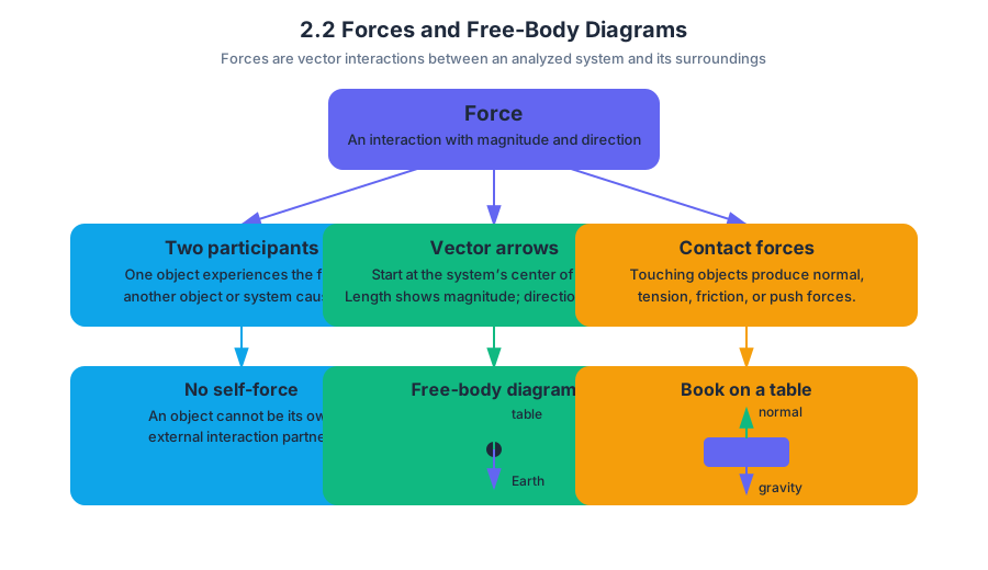
A force requires two participants: one object experiences the force, and another object or system causes it. A book resting on a table experiences an upward force from the table and a downward gravitational force from Earth. The book cannot exert a net force on itself, because an object cannot be its own external interaction partner.
Essential Knowledge 2.2.A.1: Forces are vector quantities that describe the interactions between objects or systems.
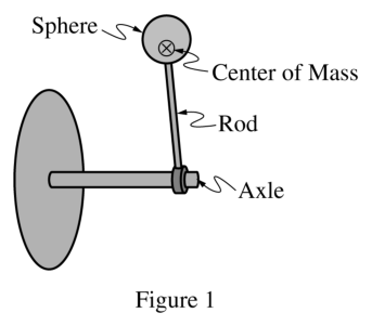
Because force is a vector, it has both magnitude and direction. A force arrow therefore needs a scale, an orientation, and a clear starting point. In a force analysis, arrows originate from the object or system being analyzed, usually represented by a dot at its center of mass.
Contact forces occur when objects or systems touch. The normal force from a floor, tension from a rope, friction from a surface, and the push from a hand are all contact forces. At the microscopic level, these are macroscopic effects of interatomic electric forces: atoms in the contacting materials resist being pushed into the same space, producing the observable interaction.
Essential Knowledge 2.2.A.1.i: A force exerted on an object or system is always due to the interaction of that object with another object or system.
Essential Knowledge 2.2.A.1.ii: An object or system cannot exert a net force on itself.
Essential Knowledge 2.2.A.2: Contact forces describe the interaction of an object or system touching another object or system and are macroscopic effects of interatomic electric forces.
Free-body diagrams isolate one system
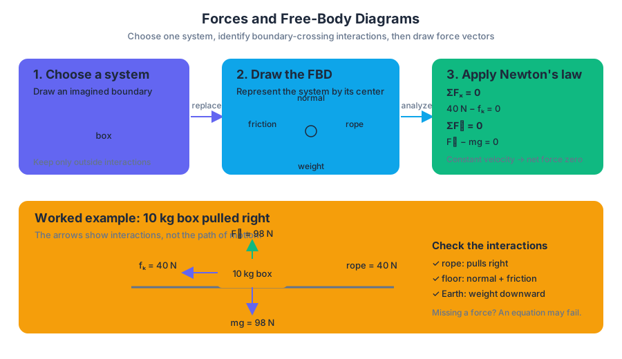
A free-body diagram is a deliberately simplified representation showing every force exerted on one chosen object or system by its environment. First draw or imagine the boundary around the system; then include only interactions that cross that boundary.
Learning Objective 2.2.B: Describe the forces exerted on an object or system using a free-body diagram.
The center-of-mass convention makes the diagram manageable: represent the system as a dot, treat its mass as concentrated at that point, and draw force vectors outward from the dot. The arrows do not show the path of motion; they show the directions of interactions.
Worked example: a box pulled across a rough floor. A $10\ \mathrm{kg}$ box is pulled horizontally to the right by a rope with force $40\ \mathrm{N}$. The floor exerts a normal force upward and kinetic friction to the left. If the box moves at constant velocity, Newton’s First Law requires zero net force:
$$\sum F_x = 0 \qquad \text{and} \qquad \sum F_y = 0.$$
Vertically, the upward normal force balances the downward weight:
$$F_N - mg = 0,$$
so
$$F_N = (10\ \mathrm{kg})(9.8\ \mathrm{m,s^{-2}})=98\ \mathrm{N}.$$
Horizontally, constant velocity means the friction force must be $40\ \mathrm{N}$ to the left:
$$40\ \mathrm{N}-f_k=0 \quad \Rightarrow \quad f_k=40\ \mathrm{N}.$$
The diagram supplies the equations. It also exposes missing interactions: if the rope is drawn but the floor’s normal force is omitted, the vertical equation cannot be justified.
Newton’s First Law: equilibrium is a force statement
Newton’s First Law states that if the net external force on a system is zero, its velocity remains constant. “Constant velocity” includes both staying at rest and moving in a straight line at unchanging speed:
$$\sum \vec{F}=0 \quad \Rightarrow \quad \vec{v}=\text{constant}.$$
This does not mean that no forces act. In the box example, several forces act, but they cancel vectorially. A stationary laptop is not force-free; its weight and the table’s normal force balance.
Misconception check — “Motion requires a net force.”
A net force is required to change velocity, not to maintain constant velocity. If friction disappeared from a sliding object, the object would continue moving with constant velocity rather than immediately stop.
Free-body diagrams versus force diagrams
A free-body diagram focuses on forces acting on a selected object or system and is used to determine translational motion. A force diagram can instead represent forces on a rigid system when analyzing the torques those forces exert. For torque, the location and line of action matter; for translational analysis, the vector sum is the central concern.
Do not place forces that the selected object exerts on its surroundings onto its own free-body diagram. Those forces belong on the diagram of the other object. This distinction prepares the paired-interaction reasoning required by Newton’s Third Law, which concerns action-reaction force pairs.
AP reasoning practices in this topic
The topic develops Science Practice 1: Creating Representations, especially Skill 1.A: Create representations of physical situations by constructing accurate free-body diagrams. It also uses Science Practice 2: Mathematical Routines, including Skill 2.D: Predict new values or factors of change of physical quantities using functional dependence between variables, such as predicting how acceleration changes when net force changes.
Students apply Skill 3.B: Apply an appropriate law, definition, theoretical relationship, or model to make a claim by using Newton’s First Law or Newton’s Second Law after drawing the diagram. They develop Skill 3.C: Justify or support a claim using evidence from experimental data, physical representations, or physical principles or laws by connecting a claim about equilibrium or acceleration to the arrows and equations.
Retrieval check
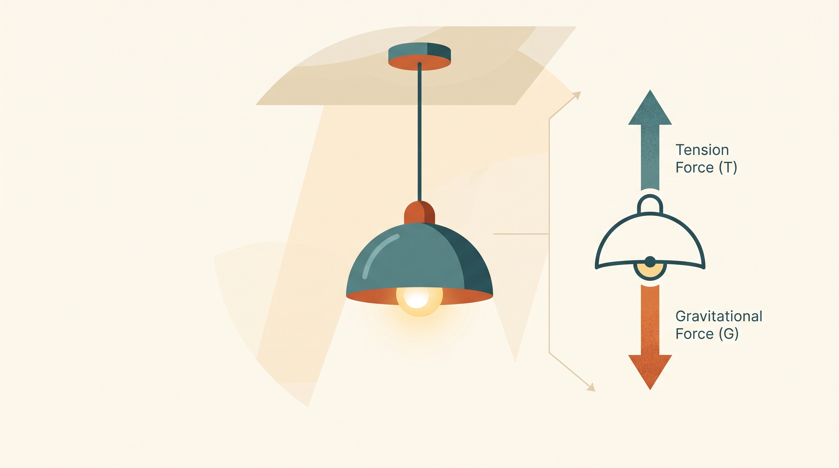
A lamp hangs motionless from a ceiling cord. Name the system, identify the forces on it, and state the net force. The correct reasoning is: for the lamp alone, the cord exerts an upward tension and Earth exerts a downward gravitational force; because the lamp is at rest, the vector sum is zero. The ceiling’s force on the cord is not placed on the lamp’s free-body diagram.
2.3 Newton’s Third Law
Key concepts: Newton’s third law · Paired forces exerted on each object · Equal-and-opposite interaction forces · Momentum changes of interacting objects · Ideal strings and tension · Strings with nonnegligible mass · Ideal pulleys · Force representations and diagrams
When a skateboard pushes backward against the ground, the ground pushes the skateboard forward with exactly the same force. Newton’s third law is not a rule about one object’s net force; it is a rule about the paired interaction between two objects.
2.3 Newton’s Third Law
When a skateboard pushes backward against the ground, the ground pushes the skateboard forward with exactly the same force. Newton’s third law is not a rule about one object’s net force; it is a rule about the paired interaction between two objects.
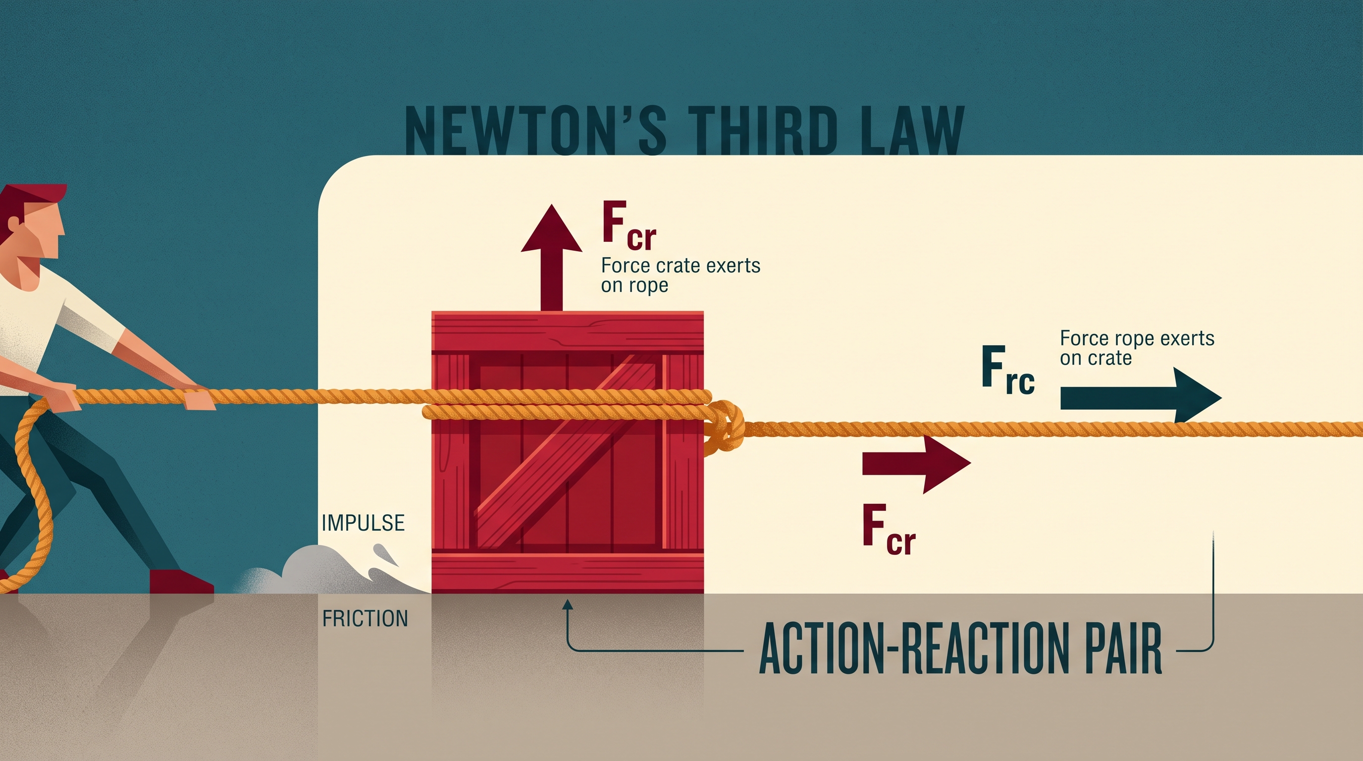
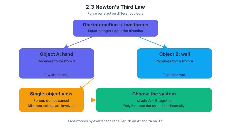
Newton’s third law: If object $A$ exerts a force on object $B$, then object $B$ exerts a force on object $A$ that has equal magnitude and opposite direction:
$$\vec{F}{\text{A on B}}=-\vec{F}{\text{B on A}}$$
Force pairs act on different objects
The two forces in a third-law pair never act on the same object. A hand pushes a wall; the wall pushes the hand. A planet pulls a satellite; the satellite pulls the planet. Because the forces act on different objects, they do not cancel on a single free-body diagram. They cancel only if both objects are included in the chosen system.
This distinction is the heart of Learning Objective 2.3.A: “Describe the interaction of two objects using Newton’s third law and a representation of paired forces exerted on each object.” A useful representation is a two-object interaction diagram:
- On object $A$: draw $\vec{F}_{\text{B on A}}$.
- On object $B$: draw $\vec{F}_{\text{A on B}}$.
- Give the arrows equal lengths and opposite directions.
- Label each force with both the object exerting it and the object receiving it.
Misconception check — “equal and opposite forces cancel.” They do not cancel when analyzing one object, because only one member of the pair acts on that object. A book resting on a table has an upward table-on-book force and a downward Earth-on-book force; these are not a third-law pair because they act on the same object. The third-law partners are table-on-book and book-on-table, or Earth-on-book and book-on-Earth.
Internal forces and momentum changes
Forces between objects inside a chosen system are internal forces. Internal forces can change the momenta of individual objects, but they do not influence the motion of the system’s center of mass, as stated in Essential Knowledge 2.3.A.2. The paired impulses are equal and opposite because impulse is force multiplied by the same interaction time:
$$\vec{J}{\text{A on B}}=\vec{F}{\text{A on B}}\Delta t=-\vec{F}{\text{B on A}}\Delta t=-\vec{J}{\text{B on A}}$$
If these paired interaction forces are the only forces contributing to the objects’ momentum changes during the same time interval, then
$$\Delta\vec{p}_A=-\Delta\vec{p}_B$$
If external forces also act, the statement must be made more carefully:
$$\Delta\vec{p}A=\vec{J}{\text{interaction on A}}+\vec{J}_{\text{external on A}}$$
and similarly for object $B$. Newton’s third law guarantees equal-and-opposite interaction impulse contributions, not necessarily equal-and-opposite total momentum changes when external impulses are present.
Worked example: a heavy block and a light block
Two blocks push apart on a nearly frictionless track. Block $1$ has much greater mass than Block $2$. During the brief interaction, assume horizontal external impulse is negligible.
Because the interaction forces are equal and opposite, the blocks receive equal and opposite impulse. Therefore,
$$\Delta\vec{p}_1=-\Delta\vec{p}_2$$
If Block $2$ has a very small change in momentum, Block $1$ also has a very small, equal-and-opposite change in momentum. Block $1$ may therefore continue traveling at approximately its original velocity. The forces are still equal; the unequal accelerations arise because
$$\vec{a}=\frac{\vec{F}_{\text{net}}}{m}$$
A small mass can undergo a large velocity change while a large mass undergoes a small velocity change under the same interaction force.
Skills in action: 1.A — Create representations, by drawing the paired-force diagram; 2.D — Predict new values or factors of change of physical quantities using functional dependence between variables, by reasoning from $\Delta v=\Delta p/m$; 3.B — Apply an appropriate law, definition, theoretical relationship, or model to make a claim, by applying Newton’s third law; and 3.C — Justify or support a claim using evidence from experimental data, physical representations, or physical principles or laws, by connecting the diagram and momentum evidence to the conclusion.
Tension in strings and cables
Tension is the macroscopic net result of forces that neighboring segments of a string, cable, chain, or similar system exert on one another in response to an external force. For an ideal string, the string has negligible mass and does not stretch under tension. Its tension is therefore the same at every point:
$$T_1=T_2=T_3=\cdots=T$$
A string with nonnegligible mass behaves differently: its tension may vary from point to point. In a hanging chain, the upper portion must support and accelerate more chain below it, so the tension is generally greater near the top. AP Physics 1 expects this variation qualitatively, not through a detailed mathematical model.
An ideal pulley has negligible mass, rotates about an axle through its center of mass, and experiences negligible friction at the axle. Under these assumptions, the pulley does not require a significant net torque to rotate, so a single ideal string passing over it has the same tension on both sides. A real massive pulley or a massive string can invalidate that shortcut.
Retrieval check
A rope pulls a crate to the right while the crate pulls the rope to the left. Are these forces a third-law pair? Yes: they act on different objects, have equal magnitude, and point in opposite directions. If the rope also experiences an external friction impulse from the floor, can you automatically conclude that the rope’s total momentum change is the negative of the crate’s? No: include that external impulse before comparing total momentum changes.
2.4 Newton’s First Law
Key concepts: Newton’s first law · Balanced and unbalanced forces · Forces balanced in one dimension but unbalanced in another · Velocity changes in the direction of the unbalanced force · Observing motion and applied forces · Bowling Ball and Broom investigation · System concept in applying Newton’s laws · Newton’s second law derived from lab data · Conservation of energy · Kinetic and potential energy
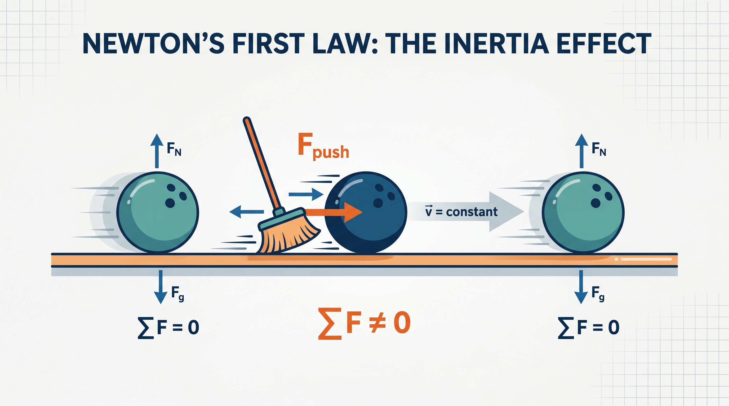
A bowling ball can keep rolling even after the broom stops pushing it. The crucial question is not “What force keeps it moving?” but “What is the net force while it moves?”
2.4 Newton’s First Law
A bowling ball can keep rolling even after the broom stops pushing it. The crucial question is not “What force keeps it moving?” but “What is the net force while it moves?”
Constant velocity means zero net force
Newton’s first law states that an object’s velocity remains constant when the net force on the system is zero:
$$\sum \vec{F}=0 \quad \Longrightarrow \quad \vec{v}=\text{constant}$$
Constant velocity includes both constant speed and constant direction. An object at rest remains at rest, while an object already moving continues in a straight line at constant speed—unless a nonzero net force changes its motion.
Key idea: Motion does not require a net force. A net force is required to change velocity.
A force can be present without producing acceleration if other forces balance it. For example, a book resting on a table has a downward gravitational force and an upward table force. These forces cancel, so the book’s velocity remains zero.
Balanced in one direction, unbalanced in another
Forces must be analyzed by components. Forces may be balanced in one dimension but unbalanced in another, and the system’s velocity changes only in the direction of the unbalanced force. This is the essential knowledge statement 2.4.A.4.
Consider a puck sliding east while a magnetic force pulls it north. If the horizontal forces balance,
$$\sum F_x=0,$$
then its eastward velocity component remains constant. If the northward force is unbalanced,
$$\sum F_y\neq 0,$$
then the puck gains a northward velocity component. Its path curves, even though there is no horizontal acceleration.
The phrase “the object accelerates” is therefore incomplete. A better claim identifies the direction:
$$\vec{a}\text{ points in the direction of }\sum\vec{F}.$$
Misconception check: “Balanced forces mean no motion”
Balanced forces mean no change in velocity, not necessarily no velocity. A spacecraft traveling far from planets can move at constant velocity with essentially zero net force. Likewise, a cart can roll at constant velocity while small resistive and driving forces cancel.
Bowling Ball and Broom investigation
In the Bowling Ball and Broom investigation, observations connect force directly to changes in motion. A broom first applies a force to a nearly stationary bowling ball. While the push acts, the ball’s velocity changes; after the broom is removed, the ball continues moving, although friction may gradually reduce its speed.
The evidence supports two linked conclusions:
- During the push, the ball experiences a nonzero net force and its velocity changes.
- After the push, if the net force is approximately zero, the ball’s velocity remains approximately constant.
A stronger push produces a larger rate of velocity change, provided the system and mass remain fixed. This observation leads toward Newton’s second law, but the first-law conclusion comes first: without an unbalanced force, the observed velocity does not change.
Choosing the system
A system is the object or collection of objects selected for analysis. For the bowling-ball observation, the system might be the ball alone. The broom, floor, Earth, and air are then outside the system and can exert external forces on it.
This choice matters because “net force” means the vector sum of forces acting on the selected system. In a modified Atwood’s machine, for example, the measured acceleration depends on whether the system is defined as one hanging mass, both masses, or the masses plus the connecting apparatus. Lab data can be used to test a relationship between net force and acceleration only after the system boundary and external forces are stated clearly.
Inertial reference frames
An inertial reference frame is a frame from which an observer verifies Newton’s first law. This is the essential knowledge statement 2.4.A.5. A laboratory floor is usually treated as approximately inertial; a rapidly turning carousel is not, because objects appear to accelerate even when no ordinary interaction force explains the motion in that frame.
AP skills in action
This topic develops four suggested skills:
- 1.C — Create qualitative sketches of graphs that represent features of a model or the behavior of a physical system. Sketch velocity as constant after the broom stops, or sketch acceleration as nonzero only while the push creates a net force.
- 2.A — Derive a symbolic expression from known quantities by selecting and following a logical mathematical pathway. Resolve forces into components and use $\sum F_x=0$ or $\sum F_y=0$ to identify which velocity component can change.
- 3.B — Apply an appropriate law, definition, theoretical relationship, or model to make a claim. Use Newton’s first law when $\sum\vec F=0$, rather than claiming that motion itself requires force.
- 3.C — Justify or support a claim using evidence from experimental data, physical representations, or physical principles or laws. Cite the bowling ball’s observed velocity before, during, and after the broom’s push.
Retrieval check: A cart moves east at constant velocity. A vertical force is added while the horizontal forces remain balanced. Which velocity component changes, and why? Answer: The vertical component changes because the net force is vertical; the eastward component remains constant because $\sum F_x=0$.

2.5 Newton’s Second Law
Key concepts: Newton’s Second Law relating net force, mass, and acceleration · Net force as the rate of change of momentum · Constant-mass form of Newton’s Second Law · Acceleration as the slope of a velocity-time graph · The relationship between net force and acceleration · The relationship between mass and acceleration · Using diagrams, tables, charts, or schematics to represent physical situations · Deriving symbolic expressions from known quantities · Applying Newton’s Second Law to motion on a rough inclined ramp · Experimental investigation of Newton’s Second Law using carts, tracks, and probeware
A velocity changes only when the net force—the vector sum of all external forces on a system—is nonzero. Newton’s Second Law turns that statement into a quantitative rule connecting force, mass, and acceleration.
2.5 Newton’s Second Law
A velocity changes only when the net force—the vector sum of all external forces on a system—is nonzero. Newton’s Second Law turns that statement into a quantitative rule connecting force, mass, and acceleration.
Learning Objective 2.5.A: Describe the conditions under which a system’s velocity changes.
From unbalanced forces to acceleration
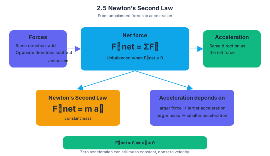
2.5.A.1: Unbalanced forces are a configuration of forces for which the net force on a system is not zero. Because force is a vector, forces pointing in opposite directions must be subtracted, while forces in the same direction add.
For a system with constant mass, Newton’s Second Law is
$$ \vec{F}_{\text{net}}=m\vec{a} $$
Equivalently,
$$ \vec{a}{\text{sys}}=\frac{\sum \vec{F}}{m{\text{sys}}} =\frac{\vec{F}{\text{net}}}{m{\text{sys}}}. $$
The acceleration points in the same direction as the net force. A larger net force produces a larger acceleration for the same mass; a larger mass produces a smaller acceleration for the same net force.
2.5.A.3: The velocity of a system’s center of mass changes only when a nonzero net external force acts on that system. Thus,
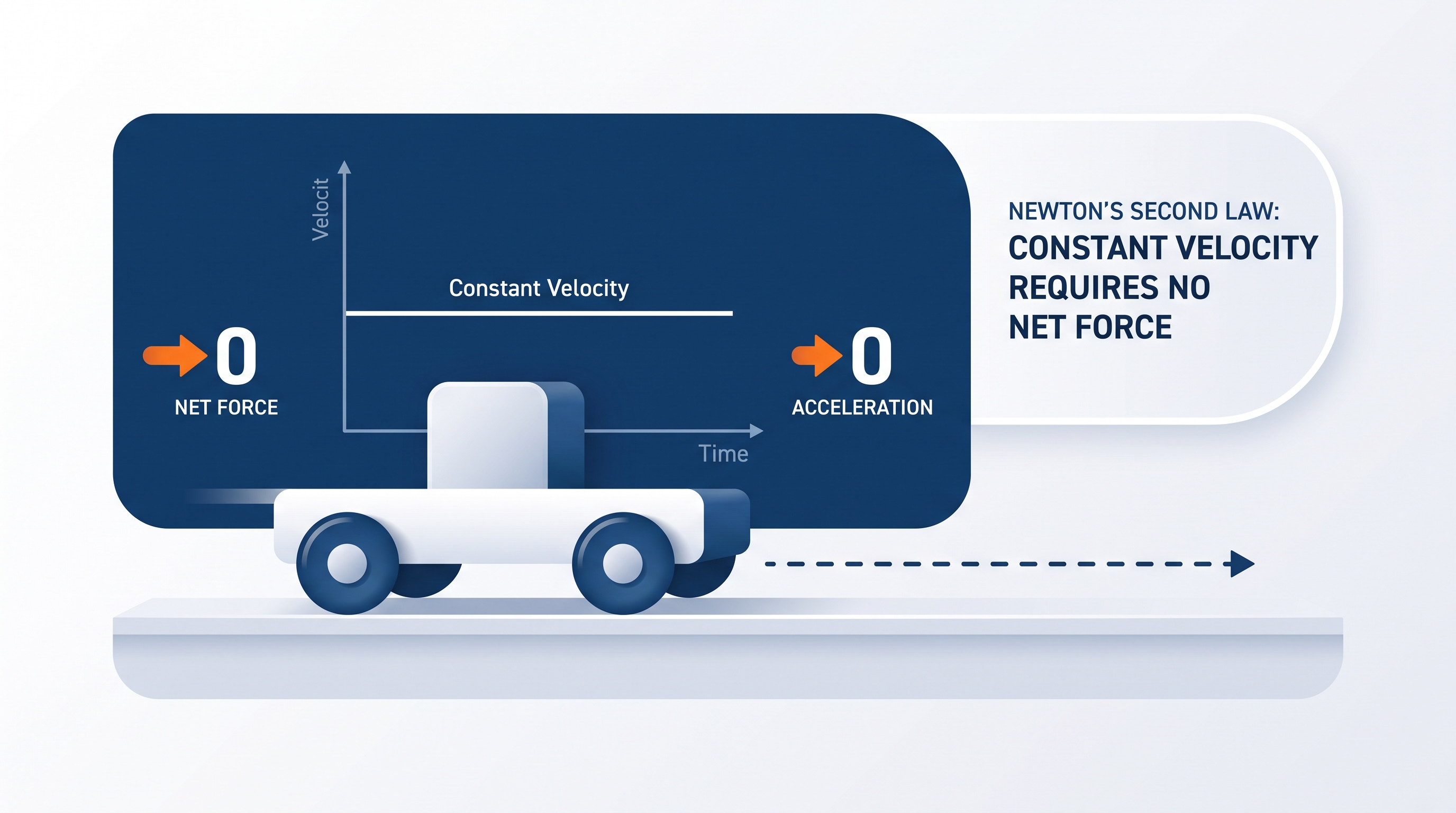
$$ \vec{F}_{\text{net}}=\vec{0} \quad\Longleftrightarrow\quad \vec{a}=\vec{0}, $$
provided the system’s mass is constant. Zero acceleration does not necessarily mean zero velocity: a cart moving at constant velocity has nonzero velocity but zero net force.
The momentum form—and the time-interval distinction
Momentum is defined as
$$ \vec{p}=m\vec{v}. $$
The change in momentum is the final momentum minus the initial momentum:
$$ \Delta\vec{p}=\vec{p}-\vec{p}_0. $$
The instantaneous, general form of Newton’s Second Law is
$$ \vec{F}_{\text{net}}=\frac{d\vec{p}}{dt}. $$
Over a finite time interval, however,
$$ \frac{\Delta\vec{p}}{\Delta t} $$
is the average net force during that interval, not necessarily the instantaneous force at every moment. If mass remains constant, then
$$ \vec{F}_{\text{net}} =m\frac{d\vec{v}}{dt} =m\vec{a}. $$
This distinction matters whenever force varies with time—for example, during a collision or while a motor gradually increases its thrust.
Reading acceleration from a velocity–time graph
Acceleration is the slope of a velocity-versus-time graph:
$$ a=\frac{\Delta v}{\Delta t} $$
for a straight segment, or the tangent slope at a particular instant on a curved graph. A horizontal segment has zero slope, so the acceleration and net force are zero at that time.
A graph that rises steadily represents constant positive acceleration and therefore a constant positive net force. A graph that slopes downward represents negative acceleration; the object may still be moving in the positive direction while slowing down.
Worked example: a block on a rough ramp
A block slides down a ramp of angle $\theta$ with kinetic-friction coefficient $\mu_k$. Choose down the ramp as positive. The forces parallel to the ramp are the downhill gravitational component $mg\sin\theta$ and the uphill friction force $f_k=\mu_k mg\cos\theta$.
The free-body representation gives
$$ \sum F_{\parallel}=mg\sin\theta-\mu_k mg\cos\theta. $$
Applying 2.5.A.2,
$$ ma=mg\sin\theta-\mu_k mg\cos\theta. $$
Divide by $m$:
$$ a=g\left(\sin\theta-\mu_k\cos\theta\right). $$
The mass cancels because both the gravitational and friction forces scale with mass. If $\theta=30^\circ$, $\mu_k=0.20$, and $g=9.8\ \text{m/s}^2$, then
$$ a=9.8\left(0.50-0.20(0.866)\right) \approx 3.2\ \text{m/s}^2. $$
If the block starts from rest and travels distance $L$, a kinematic relationship can then give its speed:
$$ v_A=\sqrt{2aL} =\sqrt{2gL\left(\sin\theta-\mu_k\cos\theta\right)}. $$
The derivation demonstrates 2.A: Derive a symbolic expression from known quantities by selecting and following a logical mathematical pathway, rather than selecting a formula by appearance.
Proportional reasoning and evidence
Under 2.D: Predict new values or factors of change of physical quantities using functional dependence between variables, inspect
$$ a=\frac{F_{\text{net}}}{m}. $$
For fixed mass, doubling $F_{\text{net}}$ doubles $a$. For fixed net force, doubling $m$ halves $a$. Under 3.B: Apply an appropriate law, definition, theoretical relationship, or model to make a claim, Newton’s Second Law supports the claim that an object speeds up only when the net force has a component in its direction of motion.
Under 1.A: Create diagrams, tables, charts, or schematics to represent physical situations, represent the situation with a force diagram, a data table, or a graph of $a$ versus $F_{\text{net}}$. A Newton’s Second Law laboratory uses carts, tracks, and probeware to vary net force and mass, measure acceleration, and test the predicted relationships. Under 3.C: Justify or support a claim using evidence from experimental data, physical representations, or physical principles or laws, the slope and pattern of the data become evidence for the model.
Misconception check
Misconception: “A force is required to keep an object moving.” A force is required to change velocity, not to maintain constant velocity. Another common error is treating $\Delta\vec{p}/\Delta t$ as the instantaneous law even when force varies; it is an interval average unless the force is constant.
Retrieval check: A cart’s velocity–time graph is horizontal at $t=4\ \text{s}$. What are its acceleration and net force at that instant? If its mass is tripled while the net force remains unchanged, what happens to its acceleration?
Answer: The graph’s zero slope means $a=0$, so $\vec{F}_{\text{net}}=\vec{0}$. Tripling the mass reduces the acceleration to one-third of its original value.
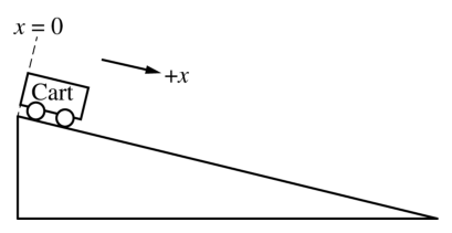
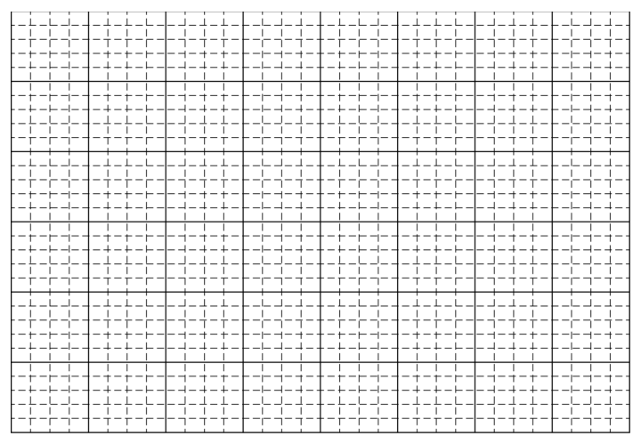
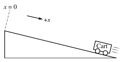
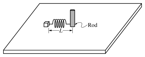
2.6 Gravitational Force
Key concepts: Gravitational field versus gravitational force · Weight as the gravitational force on an object · Apparent weightlessness · Gravitational force and circular motion · Direction of force vectors · Buoyant force versus gravitational force · Acceleration and density · Newton’s third law for internal friction forces · Gravitational potential-energy graphs · Repeated trials and reliability of measurements
A gravitational field tells you what gravity could do at a location; a gravitational force tells you what gravity does to a particular object placed there.
2.6 Gravitational Force
A gravitational field tells you what gravity could do at a location; a gravitational force tells you what gravity does to a particular object placed there. That distinction prevents one of the most common errors in force problems.
Field, force, and weight
The gravitational field strength near Earth is approximately $g = 9.8\ \mathrm{N/kg}$ downward. It is a property of the planet’s surroundings, not of the object being tested. The gravitational force on an object depends on both the field and the object’s mass:
$$ \vec F_g = m\vec g $$
Thus, a $2.0\ \mathrm{kg}$ object near Earth experiences a gravitational force of magnitude
$$ F_g = (2.0\ \mathrm{kg})(9.8\ \mathrm{N/kg}) = 19.6\ \mathrm{N}. $$
The field magnitude is $9.8\ \mathrm{N/kg}$, while the force magnitude is $19.6\ \mathrm{N}$. They are related, but they are not equal and do not even have the same units. When gravitational force is the force of Earth on an object, it is commonly called the object’s weight.
Weight is a force: $\vec W = \vec F_g = m\vec g$, directed toward the attracting planet.
Misconception check — “Weight equals $g$.”
The symbol $g$ describes the local gravitational field. Weight is $mg$. A person’s mass remains essentially constant when traveling to another planet, but the person’s weight changes if the planet produces a different gravitational field.
Direction matters on every force diagram
Gravity always points toward the attracting body. Buoyant force, by contrast, points upward in a fluid because pressure is greater at greater depth. For a submerged object, the vertical forces may be
$$ \sum F_y = F_B - F_g, $$
where $F_B$ is upward and $F_g$ is downward. If the object has volume $V$ and the fluid has density $\rho_f$, the buoyant-force magnitude is
$$ F_B = \rho_f Vg. $$
For an object of mass $m$ and density $\rho_o$, its mass can be written as $m=\rho_oV$. Therefore,
$$ \sum F_y = \rho_f Vg-\rho_o Vg = Vg(\rho_f-\rho_o), $$
and the acceleration is
$$ a_y=\frac{\sum F_y}{m} =\frac{Vg(\rho_f-\rho_o)}{\rho_oV} =g\left(\frac{\rho_f}{\rho_o}-1\right). $$
This equation shows the functional dependence clearly: acceleration depends on the ratio of fluid density to object density. Reversing the force directions would incorrectly change the sign and physical interpretation.
Misconception check — “Buoyant force and gravitational force point in the same direction.”
They oppose each other for an object immersed in a fluid. First draw the vectors; only then calculate the net force.
Apparent weightlessness
A scale does not directly measure gravitational force. It measures the contact force exerted by the scale, often called the normal force. An object appears weightless when that relevant contact force is absent, even if gravity is still acting.
For example, an astronaut orbiting Earth is continuously pulled downward by Earth’s gravity. The astronaut and spacecraft are both freely falling, so the spacecraft does not need to push upward on the astronaut. The normal force is approximately zero, producing the sensation of weightlessness.
The CED identifies this idea as 2.6.C.3: a system appears weightless when no forces act on it or when gravity is the only force acting on it. 2.6.C.4, the equivalence principle, states that an observer in a noninertial reference frame cannot distinguish between apparent weight and the gravitational force produced by a gravitational field in the appropriate local situation.
Gravity and circular motion
An orbiting object does not move in a circle because its speed is automatically “maintained.” It moves in a circle because a net force continually points toward the center. For a satellite in a circular orbit, gravity supplies the centripetal force:
$$ \frac{GMm}{r^2}=\frac{mv^2}{r}. $$
Canceling $m$ gives
$$ v=\sqrt{\frac{GM}{r}}. $$
The required circular speed is therefore smaller at larger orbital radius. Under stated conditions, an object must have at least the required speed to maintain the intended circular motion; too little speed causes the path to dip inward rather than remain on that circular path. The force vector is always radial, pointing toward the planet’s center, even though the object’s instantaneous velocity is tangent to the circle.
Representations and evidence
Near Earth, gravitational potential energy is
$$ U_g=mgh, $$
so its graph versus height is linear for constant $g$. Do not automatically treat it as the mirror image of a spring-potential-energy graph: spring energy depends on displacement squared, while gravitational energy depends linearly on vertical position. The slope of a potential-energy graph is connected to force, so the graph’s direction and steepness carry physical meaning.
In an investigation of gravitational force, repeated trials at the same location improve reliability by reducing the influence of random measurement variation. A graph of force versus mass should be consistent with $F_g=mg$; its slope represents the local gravitational field strength $g$.
The AP science practices are visible throughout this topic:
- Science Practice 1: Creating Representations — draw correctly directed force vectors, free-body diagrams, field diagrams, and force-versus-position graphs.
- Science Practice 2: Mathematical Routines — construct $\sum F$, substitute density or orbital relations, and derive functional dependence such as $a_y=g(\rho_f/\rho_o-1)$.
- Science Practice 3: Scientific Questioning and Argumentation — justify apparent weightlessness, compare planetary gravitational fields, and use repeated trials as evidence.
- Experimental Design and Analysis — identify repeated measurements as a way to improve reliability and interpret slopes.
- Qualitative/Quantitative Translation — move between “denser fluid,” vector diagrams, algebraic expressions, and predicted acceleration.
One final action-reaction reminder: if a cart exerts friction on a block, the block exerts friction of equal magnitude and opposite direction on the cart. Those forces act on different objects; they do not cancel on a single-object free-body diagram.
Retrieval check: A block is fully submerged and has $\rho_o=2\rho_f$. Which direction is its acceleration? From
$$ a_y=g\left(\frac{\rho_f}{\rho_o}-1\right) =g\left(\frac{1}{2}-1\right)=-\frac{g}{2}, $$
the acceleration is downward. The negative sign comes from assigning buoyant force upward and gravitational force downward.
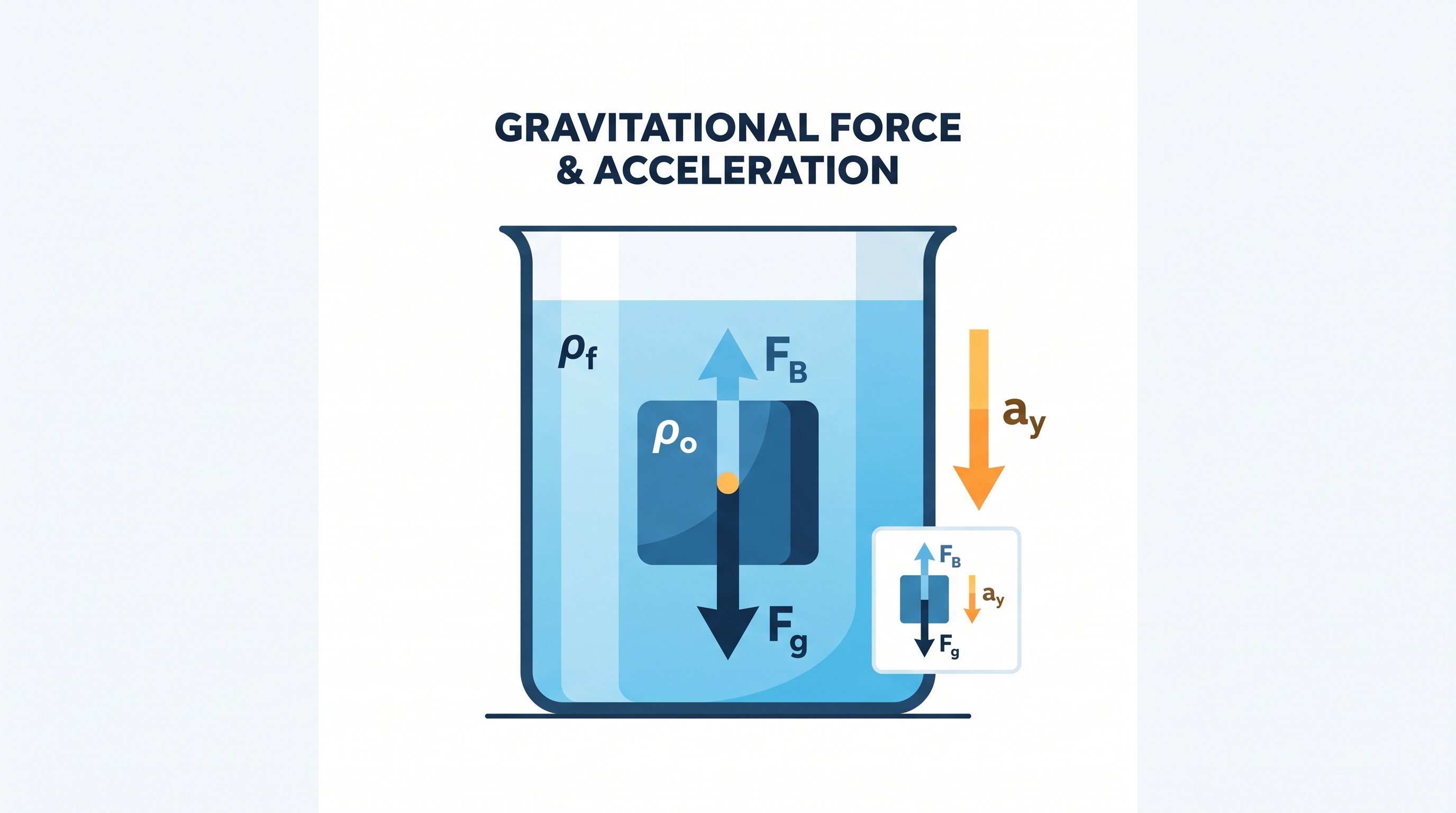
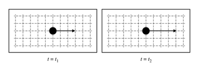
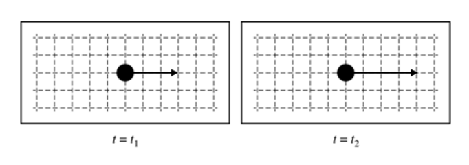
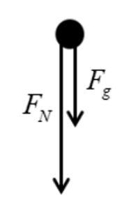
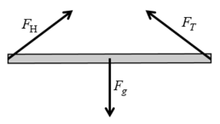
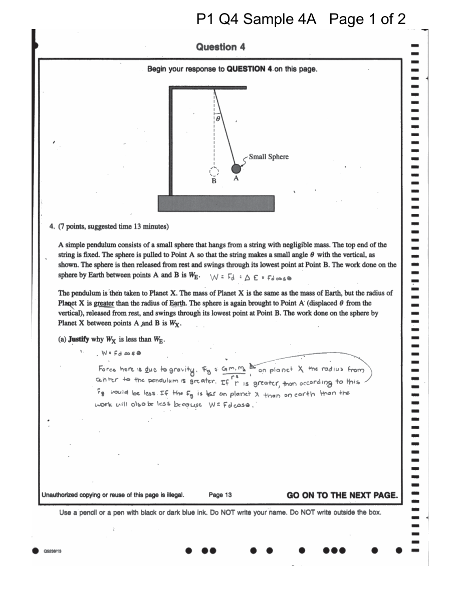
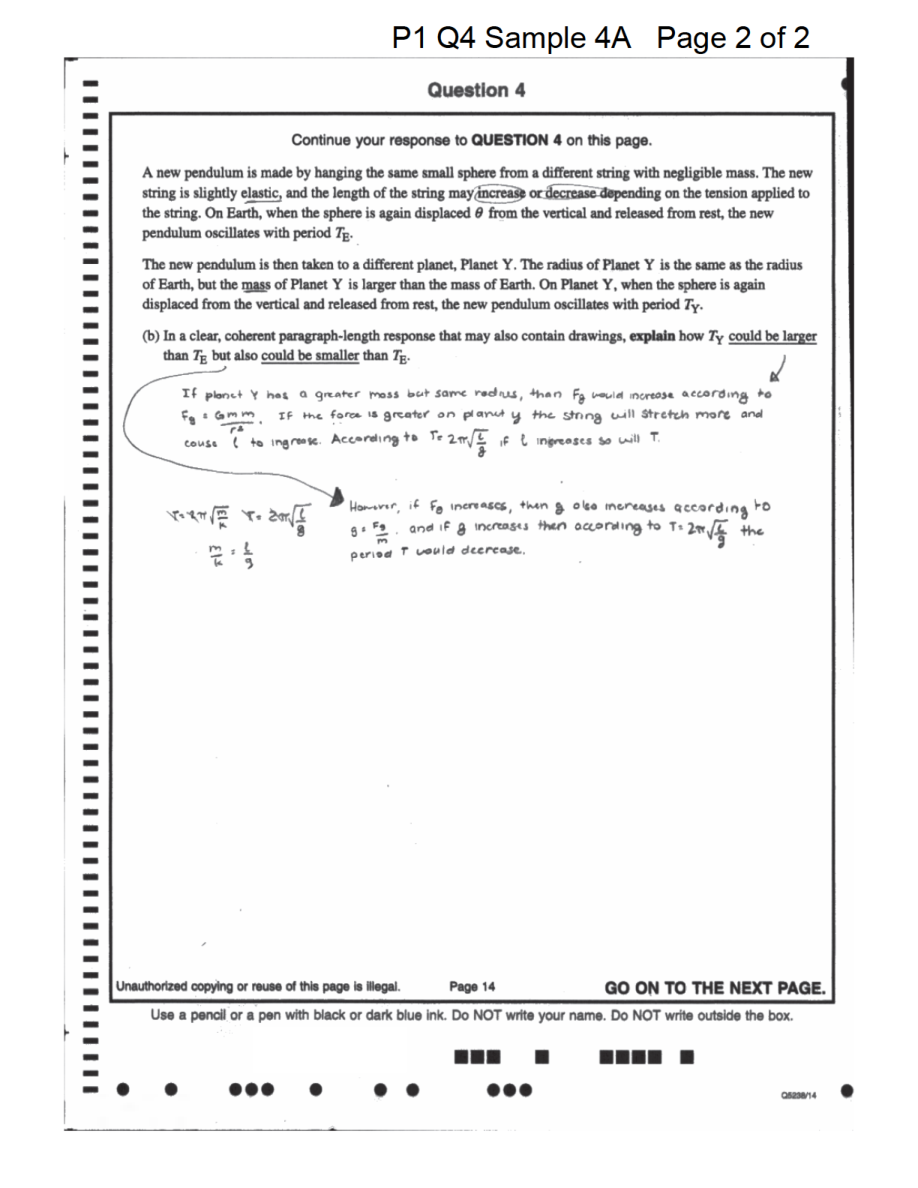
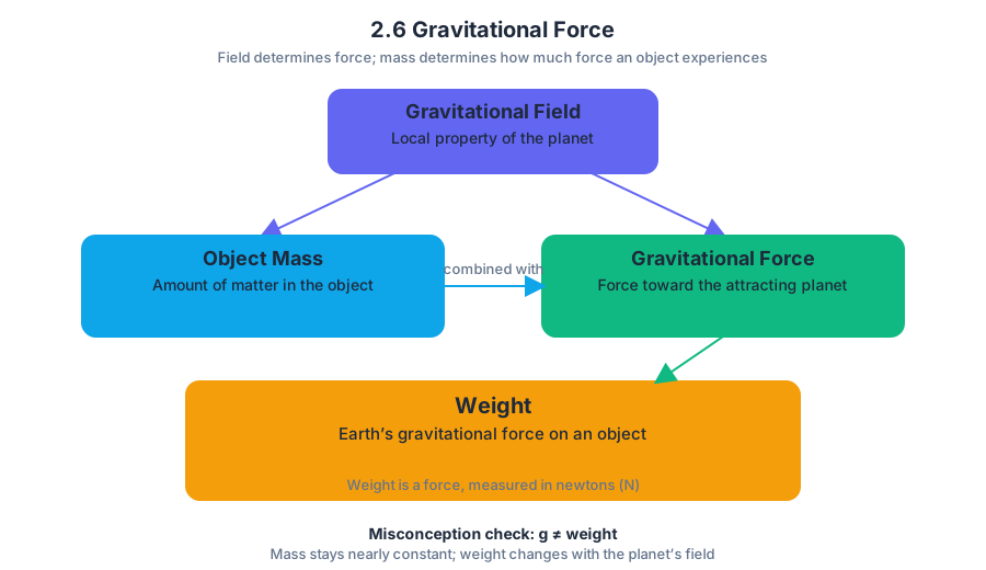
2.7 Kinetic and Static Friction
Key concepts: Kinetic friction · Static friction · Coefficient of kinetic friction · Coefficient of static friction · Normal force · Relative motion, slipping, and sliding · Independence of friction from contact area · Energy dissipation by kinetic friction · Maximum static friction · Friction in physical scenarios and comparisons
A box can remain motionless while you push it because static friction quietly matches your push—until a limiting value is reached and the box slips.
2.7 Kinetic and Static Friction
A box can remain motionless while you push it because static friction quietly matches your push—until a limiting value is reached and the box slips.
The two friction regimes
Friction is a contact force parallel to the surfaces in contact. Its direction opposes the relative motion or the attempted relative motion between those surfaces. The normal force is the perpendicular component of the force exerted by a surface on an object, directed away from the surface:
$$\vec F_n \perp \text{surface}$$
The same pair of surfaces can therefore experience two different friction models:
| Situation | Friction type | Relative motion? | Magnitude model |
|---|---|---|---|
| A shoe grips the ground without sliding | Static friction | No | $\lvert \vec F_{f,s}\rvert \leq \mu_s\lvert \vec F_n\rvert$ |
| A crate slides across the floor | Kinetic friction | Yes | $\lvert \vec F_{f,k}\rvert = \mu_k\lvert \vec F_n\rvert$ |
The vertical bars indicate magnitudes, which are nonnegative numbers. The symbols $\vec F_{f,s}$, $\vec F_{f,k}$, and $\vec F_n$ represent vector forces with directions. Friction acts along the contact surface; the normal force acts perpendicular to it.
Kinetic friction: sliding surfaces
Under 2.7.A: Describe kinetic friction between two surfaces, kinetic friction occurs when two surfaces in contact move relative to each other. Its direction is opposite the motion of each surface relative to the other surface. The coefficient of kinetic friction, $\mu_k$, describes how strongly the materials resist sliding and depends on the material properties of the surfaces in contact.
For a block sliding across a level floor, the vertical forces balance:
$$\lvert \vec F_n\rvert = mg$$
If the coefficient of kinetic friction is $\mu_k = 0.30$ and the block has mass $m = 5.0\ \mathrm{kg}$, then using $g = 9.8\ \mathrm{m/s^2}$:
$$\lvert \vec F_n\rvert = (5.0\ \mathrm{kg})(9.8\ \mathrm{m/s^2}) = 49\ \mathrm{N}$$
$$\lvert \vec F_{f,k}\rvert = \mu_k\lvert \vec F_n\rvert = (0.30)(49\ \mathrm{N}) = 14.7\ \mathrm{N}$$
The kinetic-friction force points opposite the block’s velocity relative to the floor. If the block moves right, friction points left; if it later moves left, friction reverses and points right.
A useful surprise is that this model does not depend on the size of the surface area of contact. A block resting on its broad face and the same block resting on its narrow face can have the same friction magnitude if the material pair and normal-force magnitude are unchanged.
Misconception check — “Friction always equals $\mu F_n$.”
The equation $\lvert \vec F_{f,k}\rvert = \mu_k\lvert \vec F_n\rvert$ applies to kinetic friction, when surfaces are sliding. It does not automatically describe static friction.
Static friction: gripping without slipping
Static friction occurs when two surfaces are in contact but do not move relative to each other. It is responsive, not automatically maximal: it takes whatever value is needed to prevent slipping, up to a limit:
$$\lvert \vec F_{f,s}\rvert \leq \mu_s\lvert \vec F_n\rvert$$
The largest possible static-friction magnitude is
$$\lvert \vec F_{f,s,\mathrm{max}}\rvert = \mu_s\lvert \vec F_n\rvert$$
This threshold is the boundary between gripping and slipping. Once the required friction would exceed this maximum, the surfaces begin moving relative to each other and the model changes to kinetic friction.
Suppose a $10\ \mathrm{kg}$ box rests on a level floor with $\mu_s = 0.50$. Its normal-force magnitude is
$$\lvert \vec F_n\rvert = mg = (10\ \mathrm{kg})(9.8\ \mathrm{m/s^2}) = 98\ \mathrm{N}$$
Therefore,
$$\lvert \vec F_{f,s,\mathrm{max}}\rvert = (0.50)(98\ \mathrm{N}) = 49\ \mathrm{N}$$
A horizontal applied force of $20\ \mathrm{N}$ produces static friction of $20\ \mathrm{N}$ in the opposite direction, so the box remains at rest. An applied force of $49\ \mathrm{N}$ places it at the threshold of slipping. A force greater than $49\ \mathrm{N}$ cannot be balanced by static friction, so slipping begins.
For a given pair of surfaces, the coefficient of static friction is typically greater than the coefficient of kinetic friction:
$$\mu_s > \mu_k$$
That is why starting a heavy crate is usually harder than keeping it sliding.
Energy and relative motion
Slipping and sliding mean that two surfaces move relative to each other. During this motion, the point where kinetic friction is applied moves relative to the surface, so kinetic friction transfers mechanical energy into thermal energy. Kinetic friction therefore dissipates energy from the system.
Static friction does not necessarily dissipate energy in the same way. For example, a tire rolling without slipping has a contact point that is instantaneously at rest relative to the road; static friction can change the tire’s motion without the surfaces sliding across one another.
AP reasoning tools
This topic is assessed through the following official skills:
- 1.C: Create qualitative sketches of graphs that represent features of a model or the behavior of a physical system. A friction-versus-applied-force graph rises with the applied force during static contact, reaches $\mu_s\lvert \vec F_n\rvert$, and then typically drops to the smaller kinetic value.
- 2.B: Calculate or estimate an unknown quantity with units from known quantities, by selecting and following a logical computational pathway. Determine $\lvert \vec F_n\rvert$, then apply the appropriate friction model.
- 2.C: Compare physical quantities between two or more scenarios or at different times and locations in a single scenario. Compare friction when a block is stationary, at the threshold, and sliding.
- 3.B: Apply an appropriate law, definition, theoretical relationship, or model to make a claim. Justify whether an object slips by comparing the required static friction with $\mu_s\lvert \vec F_n\rvert$.
Retrieval check: A stationary block experiences a horizontal force of $12\ \mathrm{N}$, while $\mu_s\lvert \vec F_n\rvert = 20\ \mathrm{N}$. What are the magnitude and direction of static friction? Does the block slip?
Answer: Static friction has magnitude $12\ \mathrm{N}$ opposite the applied force, and the block does not slip. The maximum value is $20\ \mathrm{N}$, but the actual static-friction force need not reach that value.
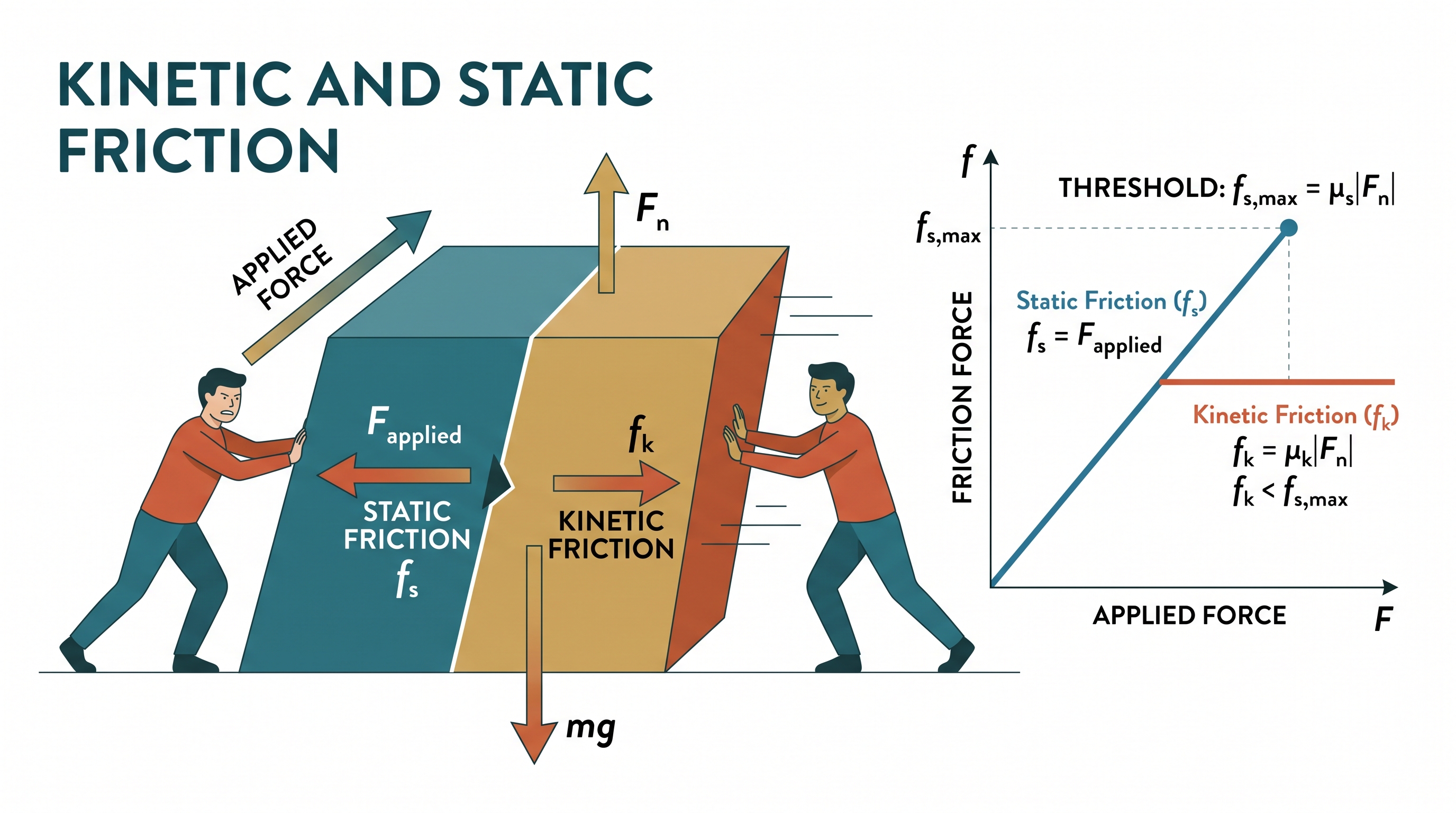
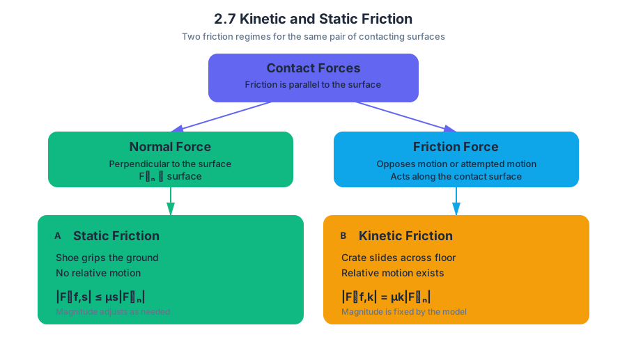
2.8 Spring Forces
Key concepts: Hooke’s law and spring force · Spring stretch and compression · Restoring force and equilibrium · Mass–spring oscillations · Force diagrams for a block attached to a spring · Centripetal force in circular motion · Radial direction of centripetal force · Relationship between spring stretch and speed · Negligible friction in spring systems · Conservation of energy in spring motion
A spring can pull a rapidly rotating block inward strongly enough to keep it moving in a circle—but only because the spring is stretched first.
2.8 Spring Forces
A spring can pull a rapidly rotating block inward strongly enough to keep it moving in a circle—but only because the spring is stretched first. The same force that points toward the center in circular motion also points back toward equilibrium when a cart oscillates.
Hooke’s law: force from displacement
For an ideal spring, the spring constant $k$ measures how difficult the spring is to stretch or compress. If the spring’s length changes by a displacement $x$ from its equilibrium length, the spring-force magnitude is
$$F_s = kx.$$
The vector form is
$$\vec F_s=-k\vec x,$$
where the minus sign means that the force points opposite the displacement. Stretch the spring to the right, and it pulls left; compress it from the left, and it pushes right.
Key idea: A spring force is a restoring force: it points toward the spring’s unstretched or equilibrium position.
In the horizontal, frictionless system considered here, with no other unbalanced horizontal force, the equilibrium position is the spring’s unstretched length $L$. More generally, natural length and equilibrium position are not automatically identical: gravity, friction, or another applied force can shift the location where the net force is zero.
Stretch, compression, and force diagrams
A block attached to a spring on a horizontal table has vertical forces that cancel: the normal force and gravitational force have equal magnitudes. The horizontal spring force is the only unbalanced force in the described system, so a correct force diagram contains one horizontal arrow for the spring force.
If the block is displaced a distance $d$ from equilibrium, the spring force has magnitude $kd$. A larger stretch or compression produces a larger force, but the length of a force arrow represents force magnitude—not the physical stretch distance. Arrows must also point in the physically correct direction.
Misconception check: “The spring force points in the direction the block is moving.”
Not necessarily. At an extreme position, the block may momentarily have zero velocity while the spring force is greatest. Direction comes from displacement, not velocity.
Mass–spring oscillations
Release a cart from rest after pulling it to one side. The spring force accelerates it toward equilibrium. The cart passes through equilibrium with its greatest speed, continues beyond equilibrium, and is then pushed back by the spring. With negligible friction, the motion repeats between
$$x=+A \qquad \text{and} \qquad x=-A,$$
where $A$ is the amplitude, the maximum displacement from equilibrium. The symbol $L$ should remain reserved for the spring’s natural length; it is not generally the oscillation amplitude.
At either endpoint, the spring is most stretched or compressed, so the spring potential energy is greatest and the cart’s kinetic energy is zero. At equilibrium, spring potential energy is smallest and kinetic energy is greatest. Because frictional forces are negligible, conservation of mechanical energy gives
$$K+U_s=\text{constant},$$
with spring potential energy
$$U_s=\frac{1}{2}kx^2.$$
The cart can therefore exchange kinetic energy and spring potential energy without changing their total.
A rotating block: spring force as centripetal force
Now attach the spring to a rod on a horizontal table and rotate the rod about its axis. When the rod is stationary, the block rests at the spring’s natural length $L$. During rotation, the spring stretches an additional distance $d$, so the block’s circular-path radius is
$$r=L+d.$$
The stretched spring pulls inward, toward the rod. That inward spring force supplies the centripetal force required for circular motion:
$$F_s=F_c,$$
so
$$kd=\frac{mv^2}{L+d}.$$
Solving for the stretch is a physical-model problem: the force grows with $d$, while the required centripetal force depends on the radius $L+d$.
For example, if $m=0.50\ \text{kg}$, $k=200\ \text{N/m}$, $L=0.40\ \text{m}$, and $v=2.0\ \text{m/s}$, then
$$200d=\frac{(0.50)(2.0)^2}{0.40+d}.$$
Multiplying through,
$$200d(0.40+d)=2.0,$$
which gives
$$d^2+0.40d-0.010=0.$$
The physically meaningful root is approximately
$$d=0.024\ \text{m}.$$
Thus the radius is $r=L+d\approx0.424\ \text{m}$.
Centripetal force is not an additional force. It is the name for the net inward force required for circular motion. Here, the spring force provides it.
The stretch can also be related to speed through energy. If a rotating block is moved between configurations without friction, the change in spring potential energy can be compared with the change in kinetic energy. In every representation—force diagram, equation, or energy argument—identify the system and the direction of the spring force before substituting numbers.
Retrieval check
A block moves in a circle while attached to a spring. Explain why the spring force is radial, then solve symbolically for the speed in terms of $k$, $d$, $m$, and $L$.
Because the spring lies along the radius from the rod to the block, its force points directly toward the rod. From
$$kd=\frac{mv^2}{L+d},$$
the speed is
$$v=\sqrt{\frac{kd(L+d)}{m}}.$$
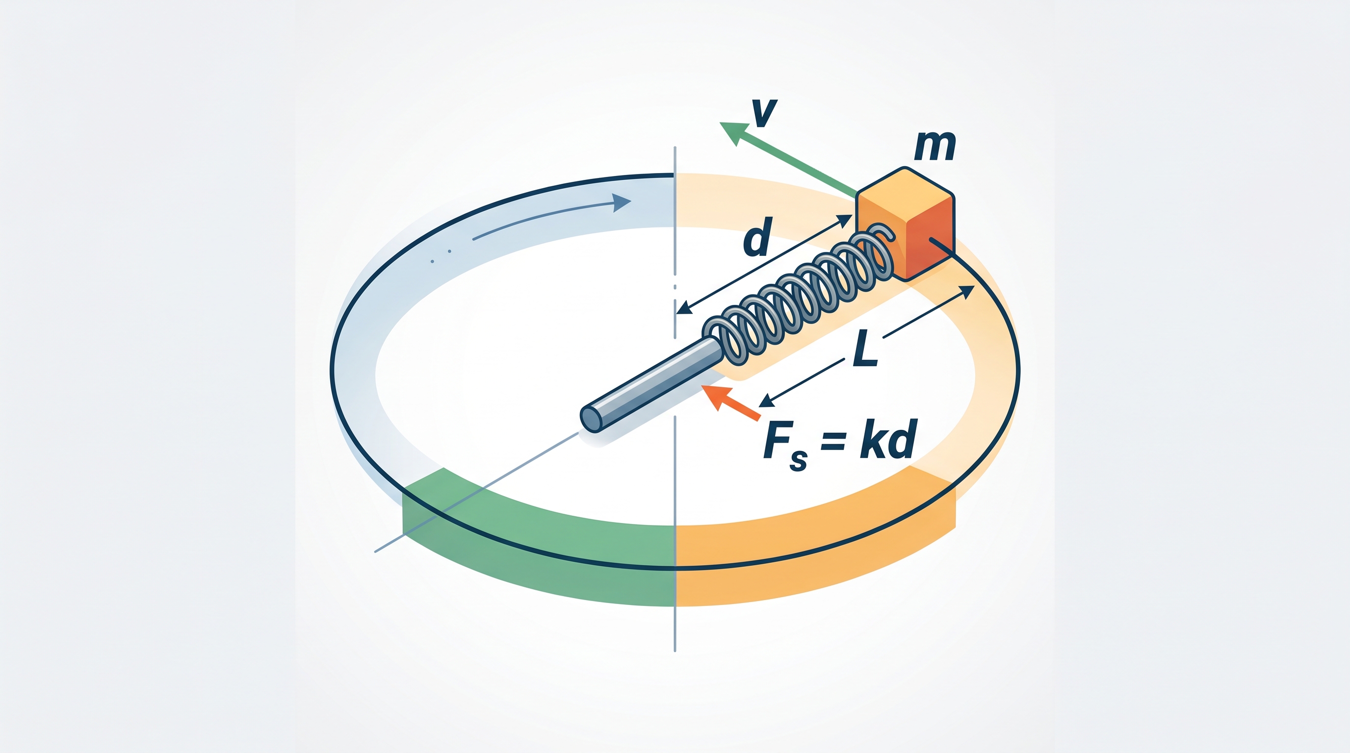
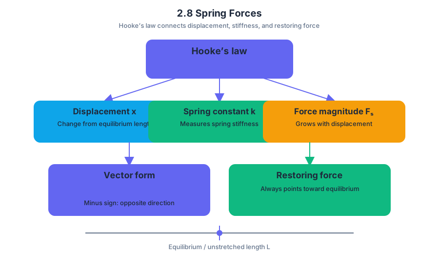
2.9 Circular Motion
Key concepts: Uniform circular motion · Centripetal force · Spring force and Hooke’s law · Tangential speed and angular speed · Radius of circular motion · Force analysis for an object moving in a circle · Motion on a frictionless horizontal table · Equilibrium and unstretched spring length · Deriving equations from force relationships · Checking qualitative and quantitative consistency
A block moving at constant speed around a circle is accelerating even when its speedometer reading never changes. The reason is that velocity includes direction, and the direction changes continuously; therefore, a net force must point toward the center of the circular path.
2.9 Circular Motion
A block moving at constant speed around a circle is accelerating even when its speedometer reading never changes. The reason is that velocity includes direction, and the direction changes continuously; therefore, a net force must point toward the center of the circular path.
A spring-powered circular-motion system
A block of mass $m_0$ is attached to a spring with spring constant $k_0$ on a frictionless horizontal table. One end of the spring connects to a central rotating rod, which a motor can turn.
Initially, the motor is off. The block is stationary, the spring is unstretched, and the distance from the rod’s center to the block is $L$. Here, $L$ is the spring’s natural length, meaning its length when it is neither compressed nor stretched.
Because the block is stationary, the horizontal forces are in equilibrium:
$$ \sum F_x = 0 $$
The spring exerts no horizontal force at this instant because its extension is zero. This initial equilibrium is different from the later rotating situation: once the spring stretches, it exerts an inward force that supplies the net force required for circular motion.
When the rod rotates, the block moves outward until the spring stretches by a distance $d$. The radius of the block’s circular path is therefore not merely $L$; it is
$$ R = L+d $$
The two distances have different meanings: $L$ is the original natural length, while $d$ is the additional stretch caused by rotation.
The inward force: centripetal force
Centripetal force is the name for the net force directed toward the center of circular motion. It is not a new kind of force. In this system, the spring force is the physical force that provides the centripetal net force.
From Hooke’s law, the stretched spring force has magnitude
$$ F_s = k_0d $$
For uniform circular motion—motion with constant tangential speed—the required inward net force is
$$ F_c = \frac{m_0v^2}{R} $$
Substituting $R=L+d$ gives
$$ F_c = \frac{m_0v^2}{L+d} $$
Since the spring is the only horizontal force on the block,
$$ F_s=F_c $$
and therefore
$$ k_0d=\frac{m_0v^2}{L+d} $$
Solving for the tangential speed $v$:
$$ v^2=\frac{k_0d(L+d)}{m_0} $$
$$ \boxed{v=\sqrt{\frac{k_0d(L+d)}{m_0}}} $$
Force analysis
A correct force diagram for the block contains:
- a normal force $N$ upward,
- a gravitational force $m_0g$ downward,
- a spring force $F_s=k_0d$ horizontally inward.
The vertical forces cancel because the table provides no vertical acceleration:
$$ N-m_0g=0 $$
The horizontal force does not cancel. It produces the inward acceleration
$$ a_c=\frac{v^2}{R} $$
so Newton’s second law becomes
$$ k_0d=m_0a_c=m_0\frac{v^2}{L+d} $$
Tangential speed and angular speed
Tangential speed $v$ measures how quickly the block moves along the circular path in meters per second. Angular speed $\omega$ measures how quickly the radius turns through an angle in radians per second.
They are related by
$$ v=\omega R $$
For this system,
$$ v=\omega(L+d) $$
Thus, two blocks can have the same angular speed but different tangential speeds if they move at different radii. The block farther from the center travels a greater distance during each revolution.
Reading the equation qualitatively
The derived equation gives more than a numerical answer. Holding $k_0$, $d$, and $m_0$ fixed,
$$ v=\sqrt{\frac{k_0d}{m_0}}\sqrt{L+d} $$
so
$$ v\propto\sqrt{L+d} $$
Increasing the radius increases the required tangential speed according to a square-root relationship. For example, if $L+d$ becomes four times larger while the other quantities remain fixed, the predicted speed becomes twice as large—not four times as large.
This is a qualitative-to-quantitative consistency check: a verbal prediction about how changing a variable affects motion must agree with the mathematical dependence in the derived equation.
Spring energy is not spring force
The stretched spring also stores elastic potential energy:
$$ U_s=\frac{1}{2}k_0d^2 $$
This quantity is measured in joules and describes stored energy. The spring force,
$$ F_s=k_0d $$
is measured in newtons and describes the instantaneous interaction that pulls the block inward. Confusing these expressions produces a dimensional error: $k_0d$ can be a force, whereas $\frac{1}{2}k_0d^2$ is an energy.
Key distinction: $F_s=k_0d$ supplies the centripetal force; $U_s=\frac{1}{2}k_0d^2$ describes energy stored in the stretched spring.
Misconception check
Misconception: “Centripetal force” is an additional force alongside the spring force.
Correction: centripetal force is the inward net-force role. Here, the spring force fills that role.
Misconception: The block moves outward because an outward force keeps it in the circle.
Correction: on the frictionless table, the horizontal spring force points inward. The block’s tendency to continue in a straight line is balanced by this inward force, producing circular motion.
Misconception: A larger radius automatically means a larger speed.
Correction: the conclusion depends on what is held fixed. The equation above shows $v\propto\sqrt{L+d}$ only when $k_0$, $d$, and $m_0$ are unchanged.
AP reasoning in this model
This problem directly exercises Science Practice 1—Creating Representations, especially 1.A (representing a physical situation) through the labeled setup and force diagram; Science Practice 2—Mathematical Routines, especially 2.A (using algebraic relationships) and 2.B (calculating a physical quantity); and Science Practice 3—Scientific Questioning and Argumentation, especially 3.A (making a claim supported by evidence). The evidence for a claim about increased speed is the functional relationship $v\propto\sqrt{L+d}$, not merely an unsupported verbal assertion.
Retrieval check: If the spring suddenly became slack while the block was moving, which way would the block initially travel, and which equation identifies the inward force before that happens?
The block would initially travel tangent to the circle, because its instantaneous velocity is tangential. Before the spring becomes slack, the inward force is identified by
$$ F_s=k_0d=\frac{m_0v^2}{L+d} $$
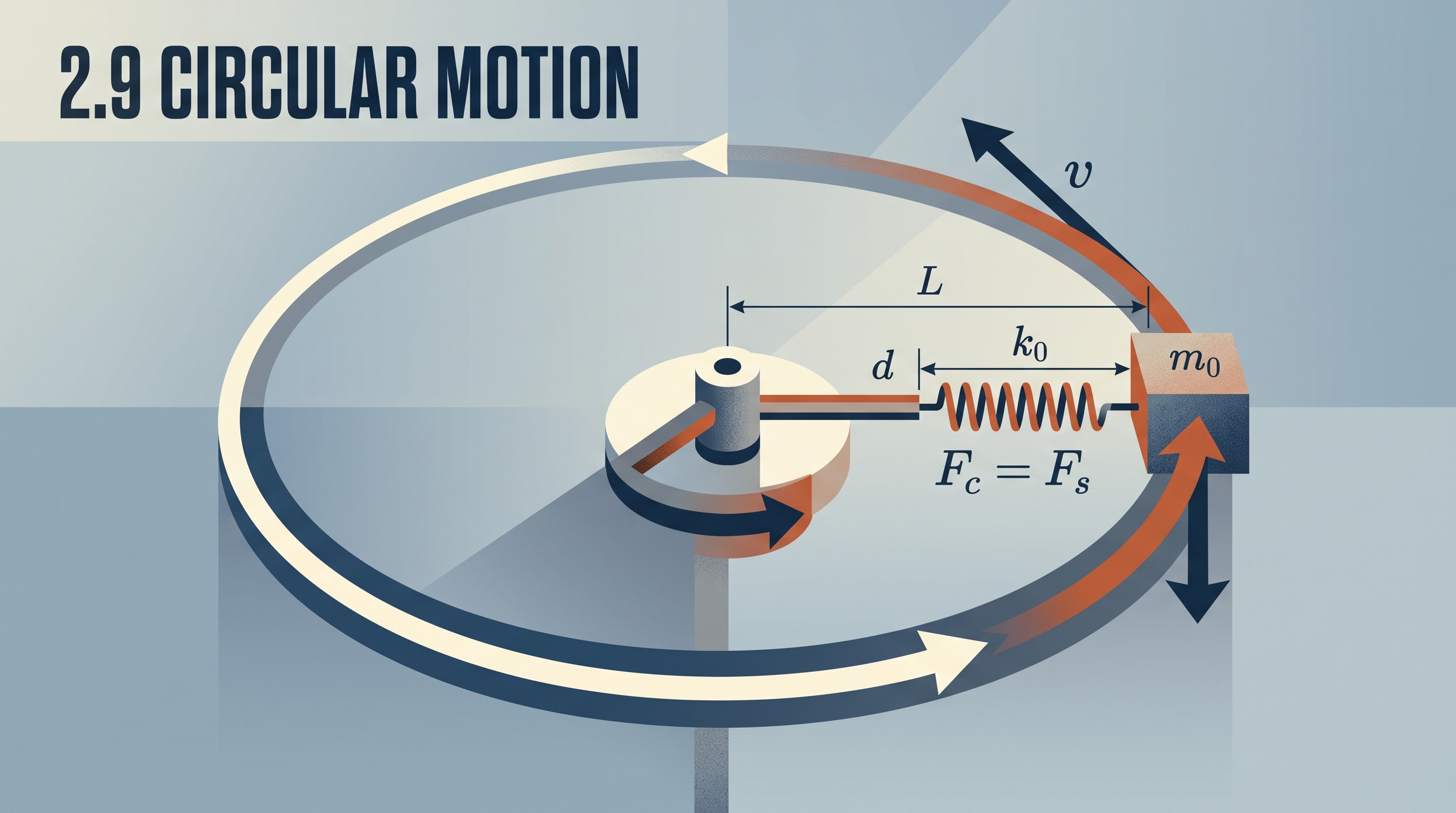
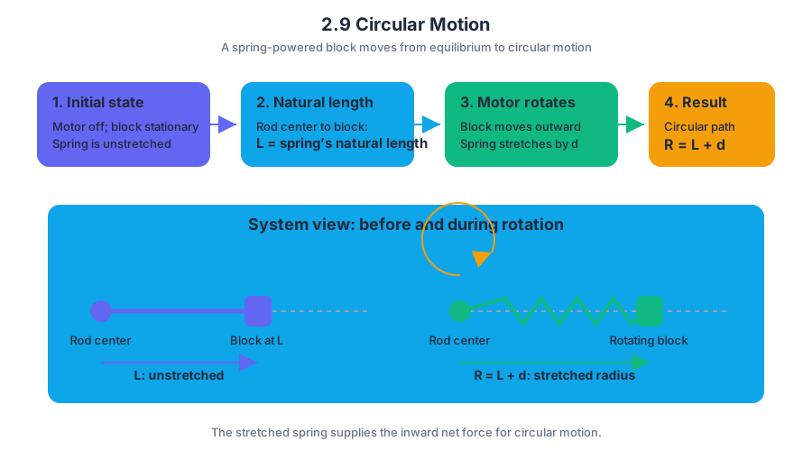
3.1 Translational Kinetic Energy
Key concepts: Translational kinetic energy · Linear motion of an object's center of mass · Mass · Velocity (speed) · Scalar quantity
An object has translational kinetic energy when its center of mass moves from one place to another. A rolling bicycle, a sliding book, and a spacecraft traveling through space all possess translational kinetic energy because their overall motion is linear, even if the objects also rotate.
3.1 Translational Kinetic Energy
An object has translational kinetic energy when its center of mass moves from one place to another. A rolling bicycle, a sliding book, and a spacecraft traveling through space all possess translational kinetic energy because their overall motion is linear, even if the objects also rotate.
Translational kinetic energy is the energy associated with the linear motion of an object’s center of mass.
The center of mass is the single location that represents the object’s overall distribution of mass. For many ordinary problems, it moves as though all the object’s mass were concentrated at that point. Thus, the translational kinetic energy describes the motion of the object as a whole, not the detailed motion of every individual particle within it.
The mathematical model
The translational kinetic energy of an object depends on its mass and its velocity:
$$ K = \frac{1}{2}mv^2 $$
Here, $K$ is translational kinetic energy, measured in joules ($\text{J}$), $m$ is mass in kilograms ($\text{kg}$), and $v$ is the object’s speed in meters per second ($\text{m/s}$). Although the formula uses the symbol $v$ for velocity, the squared quantity $v^2$ means that the energy depends on the velocity’s magnitude, or speed.
The equation reveals two important scaling rules:
- If the mass doubles while the speed stays constant, $K$ doubles.
- If the speed doubles while the mass stays constant, $K$ becomes four times as large because $(2v)^2 = 4v^2$.
That squared dependence makes speed especially important in collisions and transportation safety. Increasing a vehicle’s speed from $10\ \text{m/s}$ to $20\ \text{m/s}$ does not merely double its translational kinetic energy; it quadruples it.
Worked example: comparing two carts
A laboratory cart has mass $m = 2.0\ \text{kg}$ and moves at speed $v = 3.0\ \text{m/s}$. Its translational kinetic energy is
$$ K = \frac{1}{2}mv^2 $$
$$ K = \frac{1}{2}(2.0\ \text{kg})(3.0\ \text{m/s})^2 $$
$$ K = 9.0\ \text{J} $$
Now consider a second cart with the same mass moving at $6.0\ \text{m/s}$. Because its speed is twice as great,
$$ K_2 = \frac{1}{2}(2.0\ \text{kg})(6.0\ \text{m/s})^2 = 36\ \text{J} $$
The second cart has four times the kinetic energy, not twice the kinetic energy. A useful AP strategy is to compare ratios before calculating:
$$ \frac{K_2}{K_1} = \left(\frac{v_2}{v_1}\right)^2 = \left(\frac{6.0}{3.0}\right)^2 = 4 $$
Kinetic energy is scalar
Translational kinetic energy is a scalar quantity, meaning it has magnitude but no direction. Velocity is a vector, so an object moving east and an identical object moving west have opposite velocities. However, if they have the same mass and speed, they have the same translational kinetic energy:
$$ K_{\text{east}} = \frac{1}{2}m(+v)^2 = \frac{1}{2}mv^2 $$
$$ K_{\text{west}} = \frac{1}{2}m(-v)^2 = \frac{1}{2}mv^2 $$
The negative sign disappears when velocity is squared. This does not mean direction never matters in physics; direction matters greatly for vector quantities such as velocity, acceleration, force, and momentum. It means only that direction does not change the value of kinetic energy for a given mass and speed.
Common misconception — “Kinetic energy can be negative.”
Translational kinetic energy cannot be negative because $m$ is positive and $v^2$ is never negative. A negative velocity can describe direction, but it still produces positive kinetic energy.
Reference frames matter
Different observers can measure different translational kinetic energies for the same object because they may measure different speeds. A passenger sitting inside a train may measure a backpack’s speed as $0\ \text{m/s}$, giving $K = 0$. An observer standing beside the track measures the same backpack moving with the train and therefore measures a nonzero kinetic energy.
The equation itself has not changed; the measured velocity has. Always identify the observer’s reference frame before comparing kinetic energies.
AP skill connection
This topic directly develops 1.A: Create representations. A motion sketch should label the center of mass, show the chosen positive direction, and identify the measured speed. It also develops 2.B: Calculate or estimate an unknown quantity with units from known quantities, by selecting and following a logical computational pathway: identify $m$ and $v$, substitute into $K = \frac{1}{2}mv^2$, and report joules.
Retrieval check: Two identical balls have equal speeds, but one travels north and the other travels south. Which has greater translational kinetic energy? Neither: their kinetic energies are equal because kinetic energy depends on mass and $v^2$, not on the direction of velocity.
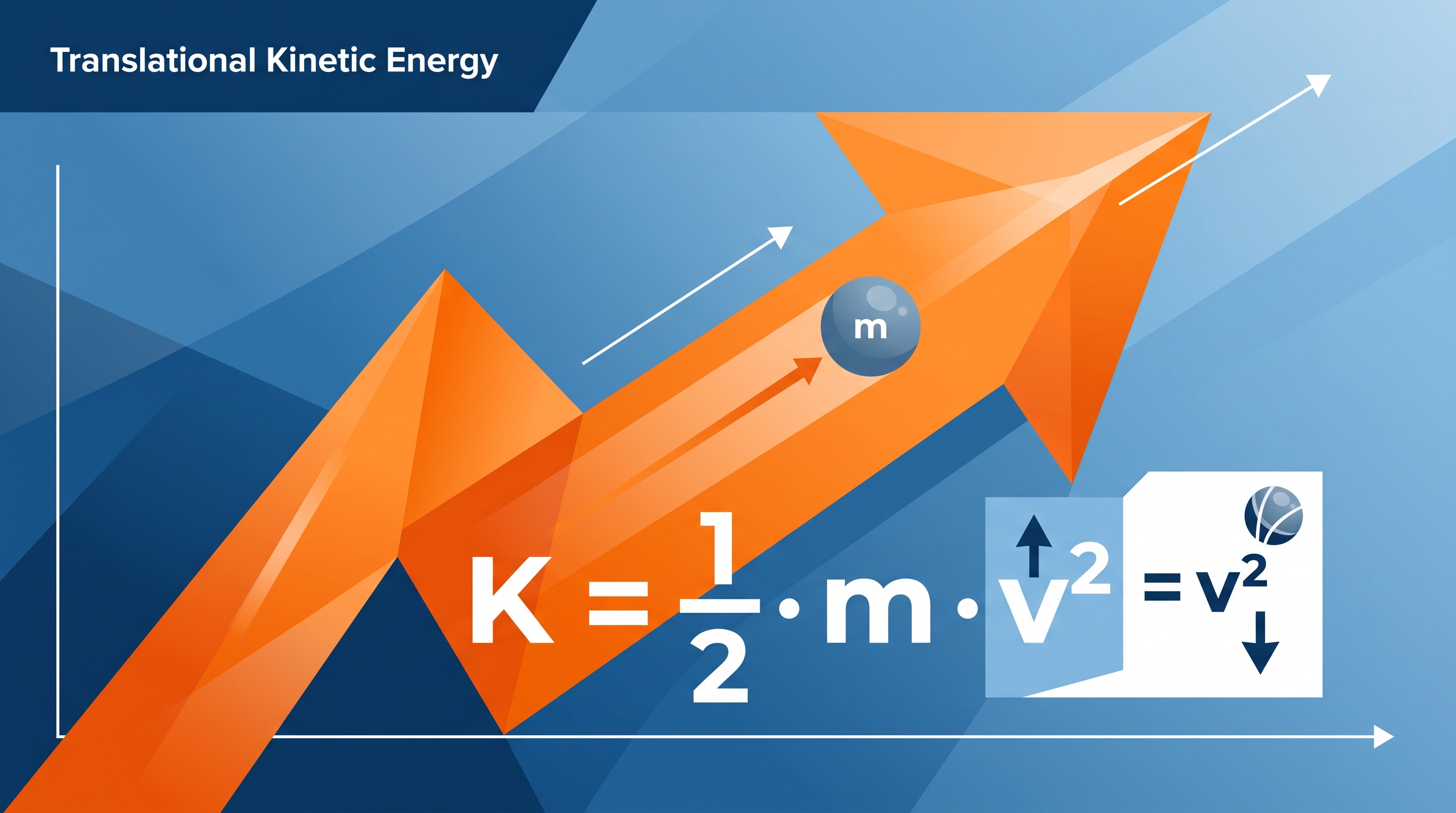
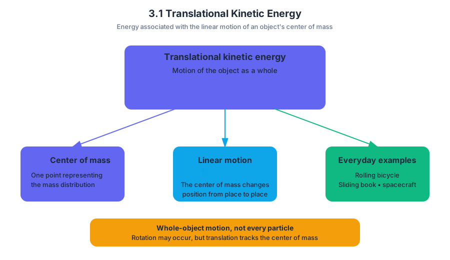
3.2 Work
Key concepts: Sphere · Tangent (tan) · Variable v representing speed
A force does work when it transfers energy to or from a system through a displacement. Pushing a motionless wall can feel exhausting, but if the wall does not move, the wall does not receive mechanical work from your push.
3.2 Work
A force does work when it transfers energy to or from a system through a displacement. Pushing a motionless wall can feel exhausting, but if the wall does not move, the wall does not receive mechanical work from your push.
The work done by a constant force
For a constant force, work depends on three ingredients: the force magnitude $F$, the displacement magnitude $d$, and the angle $\theta$ between them.
$$ W = Fd\cos\theta $$
The factor $\cos\theta$ selects the component of the force parallel to the displacement. A force pointing along the motion transfers the most energy; a force perpendicular to the motion transfers none.
| Force–displacement relationship | Angle $\theta$ | Work |
|---|---|---|
| Force and displacement point in the same direction | $0^\circ$ | $W=Fd$ |
| Force is perpendicular to displacement | $90^\circ$ | $W=0$ |
| Force opposes displacement | $180^\circ$ | $W=-Fd$ |
| Force acts at an arbitrary angle | $\theta$ | $W=Fd\cos\theta$ |
Work is a scalar, meaning it has magnitude and sign but no direction of its own. The sign matters: positive work transfers energy into the system’s motion, while negative work removes energy from it.
Key definition: Work is the product of the force component parallel to the displacement and the displacement itself.
Worked example: pulling a sphere
A student pulls a small sphere across a level table with a constant force of $12\ \mathrm{N}$ directed $30^\circ$ above the horizontal. The sphere moves $4.0\ \mathrm{m}$ horizontally. How much work does the pulling force do?
Only the horizontal component of the force contributes:
$$ F_{\parallel}=F\cos\theta $$
Therefore,
$$ W=Fd\cos\theta $$
$$ W=(12\ \mathrm{N})(4.0\ \mathrm{m})\cos(30^\circ) $$
$$ W\approx 41.6\ \mathrm{J} $$
The answer is approximately $42\ \mathrm{J}$. The upward component of the pull does no work because the sphere’s displacement is horizontal. The normal force and gravitational force are also perpendicular to the displacement, so each does zero work in this idealized motion.
Angles, components, and the tangent function
When a force direction is described using horizontal and vertical components, trigonometry identifies its angle. If the horizontal component is $a$ and the vertical component is $b$, then
$$ \tan\theta=\frac{b}{a} $$
or equivalently,
$$ a\tan\theta=b $$
This angle must be interpreted carefully: in the work equation, $\theta$ is the angle between the force and the displacement, not necessarily the angle between the force and the floor in every diagram. Drawing the force vector and displacement vector first prevents the most common angle error.
Work and changes in speed
The previously established kinetic-energy result connects work to motion through the work–energy theorem:
$$ W_{\text{net}}=\Delta K $$
Here, $v$ represents speed, the magnitude of velocity. Because translational kinetic energy depends on $v^2$, positive net work increases speed, negative net work decreases speed, and zero net work leaves speed unchanged—even if individual forces are present.
For example, if a pulling force does $42\ \mathrm{J}$ of positive work while friction does $18\ \mathrm{J}$ of negative work, the net work is
$$ W_{\text{net}}=42\ \mathrm{J}-18\ \mathrm{J}=24\ \mathrm{J} $$
The system therefore gains $24\ \mathrm{J}$ of kinetic energy. Notice that the work done by one force is not automatically the work responsible for the change in speed; the relevant quantity is the sum of the work done by all external forces.
Misconception check: “A force always does work”
Correction: A force does work only when it has a component along the displacement. Carrying a backpack at constant height while walking forward involves an upward force from your arms and a horizontal displacement, so that supporting force does approximately zero mechanical work on the backpack. In contrast, friction opposing the backpack’s motion would do negative work.
AP Science Practices in this topic
- Science Practice 1: Creating Representations — draw force and displacement vectors, identify $\theta$, and translate a physical situation into $W=Fd\cos\theta$.
- Science Practice 2: Mathematical Routines — resolve components, use $\cos\theta$ or $\tan\theta$, track signs, and report work in joules.
- Science Practice 3: Scientific Questioning and Argumentation — justify whether a force does positive, negative, or zero work using the force–displacement geometry and evidence from motion.
Retrieval check: A $20\ \mathrm{N}$ force acts at $60^\circ$ to a displacement of $3.0\ \mathrm{m}$. Calculate the work done by that force.
$$ W=(20)(3.0)\cos(60^\circ)=30\ \mathrm{J} $$
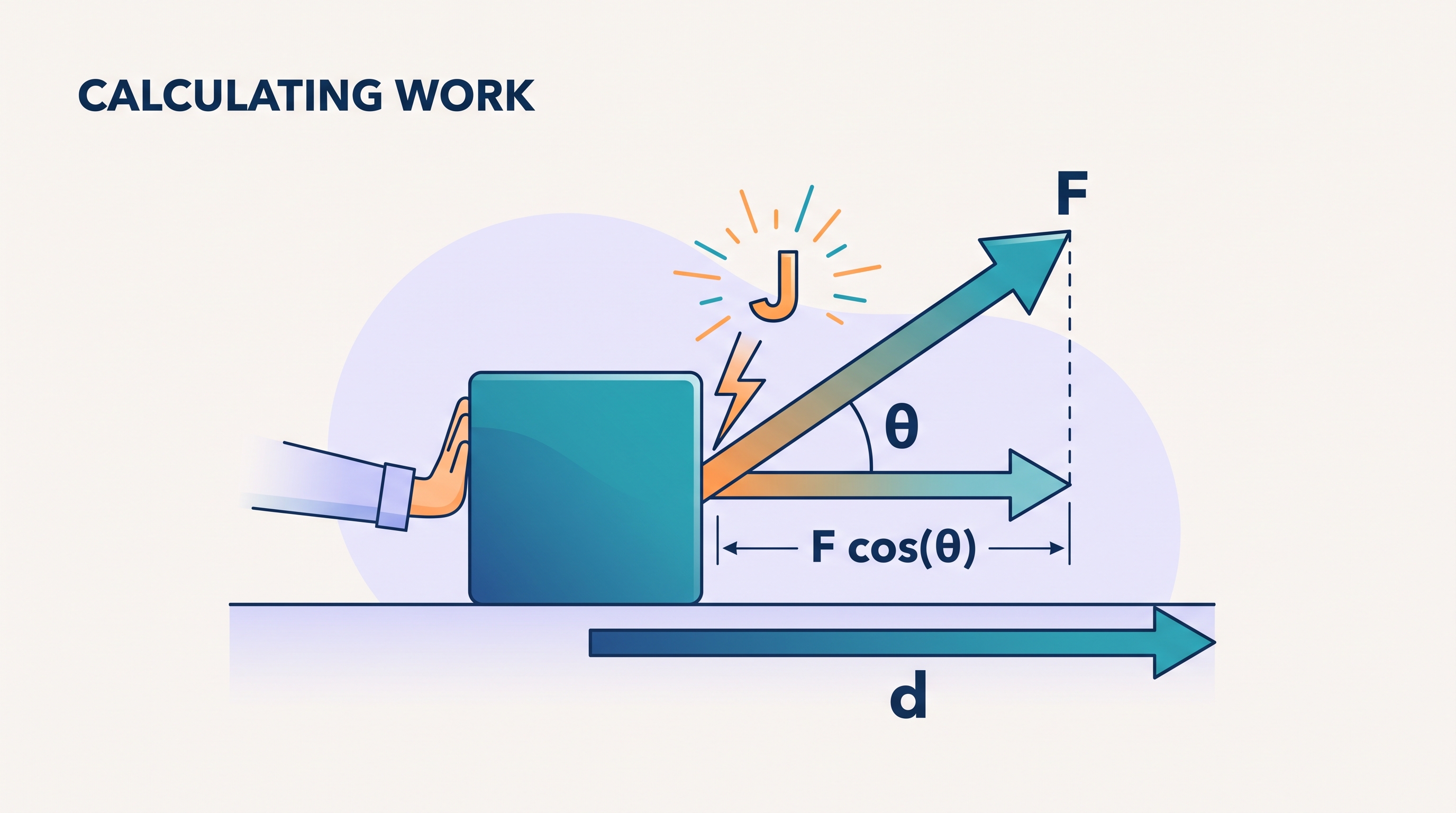
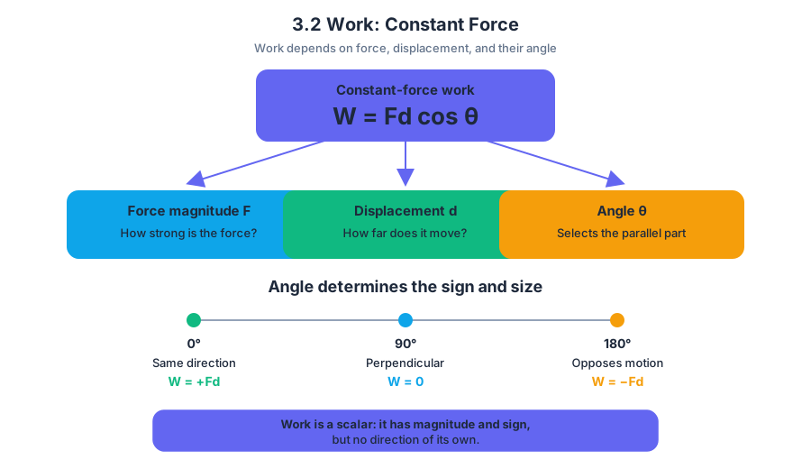
3.3 Potential Energy
Key concepts: Potential energy associated with conservative forces · Conservation of mechanical energy · Gravitational potential energy · Elastic spring potential energy · Kinetic energy and energy bar charts · Thermal energy from friction · Energy transformations in multi-component systems · Total mechanical energy versus position · Using geometric displacement on an incline · Comparing energy and speed at different positions
A compressed spring, a raised block, and a sliding object can all store energy in different ways—but only certain forces allow that stored energy to be recovered without depending on the path taken.
3.3 Potential Energy
A compressed spring, a raised block, and a sliding object can all store energy in different ways—but only certain forces allow that stored energy to be recovered without depending on the path taken. Potential energy is energy associated with the arrangement of interacting objects.
Conservative forces: energy that remembers only position
A conservative force is a force whose work depends only on the initial and final positions, not on the route between them. Gravity is conservative: lifting a book by $0.50\ \text{m}$ requires the same change in gravitational potential energy whether the book moves straight upward or along a winding path.
For a conservative force, the work done by that force equals the negative change in potential energy:
$$W_{\text{conservative}}=-\Delta U$$
The minus sign means that when a conservative force does positive work, the associated potential energy decreases. As a block falls, gravity does positive work while $U_g$ decreases; as a spring is compressed, the external agent does work that increases $U_s$.
Over a closed path, an object returns to its starting position, so the net work done by a conservative force is zero and the potential-energy change is also zero:
$$W_{\text{closed path}}=0,\qquad \Delta U_{\text{closed path}}=0$$
Gravitational potential energy
Near Earth’s surface, gravitational potential energy is determined by vertical position:
$$U_g=mgh=mg\Delta y$$
Here, $m$ is mass, $g$ is the magnitude of the gravitational field, and $\Delta y$ is the change in vertical position. The zero level for $U_g$ is arbitrary; changing it shifts every gravitational-potential value by the same amount but does not change measurable motion.
For a block moving a distance $d$ along an incline at angle $\theta$, the vertical displacement is not $d$. Geometry gives
$$\Delta y=d\sin\theta$$
so the gravitational-potential-energy change is
$$\Delta U_g=mgd\sin\theta$$
For example, a $2.0\ \text{kg}$ block moves $3.0\ \text{m}$ up a $30^\circ$ incline. Its vertical rise is
$$\Delta y=(3.0\ \text{m})\sin 30^\circ=1.5\ \text{m}$$
Thus,
$$\Delta U_g=(2.0)(9.8)(1.5)\ \text{J}=29.4\ \text{J}$$
Misconception check — distance along the ramp is height. The block travels $3.0\ \text{m}$, but it rises only $1.5\ \text{m}$. Gravitational potential energy responds to vertical displacement, not path length.
Elastic spring potential energy
A spring stores energy when its length differs from its relaxed length. If $x$ is the compression or stretch magnitude and $k$ is the spring constant, the stored elastic potential energy is
$$U_s=\frac{1}{2}kx^2$$
The square matters: doubling the deformation quadruples the stored energy. The energy is the same for compression and extension of equal magnitude in the ideal spring model.
Mechanical energy can move among translational kinetic energy, gravitational potential energy, and spring potential energy:
$$E_{\text{mechanical}}=K+U_g+U_s$$
When no friction or other nonconservative energy transfer is present, the total remains constant. A falling object may convert $U_g$ into $K$; a spring launcher may convert $U_s$ into $K$; a block moving downward toward a spring may distribute energy among all three forms.
Energy bar charts and energy-versus-position graphs
An energy bar chart is a representation, not a picture of the object. Include only the energy forms specified for the system. For a system containing a block and Earth, a position might require only a $U_g$ bar; at another position, the chart might contain only $K$ and $U_g$.
In one worked representation, the total energy is $12E_0$. At $x=0$, the system has $U_g=12E_0$, with $K=0$ and $U_s=0$. At $x=6D$, the bars can be $K=6E_0$ and $U_g=6E_0$, still totaling $12E_0$.
The same reasoning appears on an energy-versus-position graph. If mechanical energy is conserved, the total-energy graph is horizontal. In the stated example,
$$E=12E_0$$
from $x=8D$ to $x=12D$. Gravitational potential energy decreases linearly with position when the object moves down a straight incline at constant angle.
Comparing positions by total potential energy
At $x=9D$, suppose the gravitational potential energy is $U_g=3E_0$, while the spring potential energy is less than $E_0$. Since the total is $12E_0$,
$$K=12E_0-U_g-U_s$$
Because $U_s<E_0$,
$$K>12E_0-3E_0-E_0=8E_0$$
More than $8E_0$ remains as kinetic energy. The conclusion does not require knowing the exact spring energy.
If two positions in a conservative system have the same total potential energy,
$$U_{\text{total},1}=U_{\text{total},2}$$
then conservation of mechanical energy requires equal kinetic energies:
$$K_1=K_2$$
For the example, this means equal speeds at $x=8D$ and $x=9D$ only if the total potential energy is equal at those positions—not merely one component such as $U_g$.
Friction and thermal energy
Friction is nonconservative. It transforms mechanical energy into thermal energy, so $K+U_g+U_s$ decreases even though energy is not destroyed. Whether the mechanical energy of a system increases, decreases, or remains constant depends on the system boundary: excluding Earth can make gravity an external energy transfer, while including Earth places gravitational potential energy inside the system.
Retrieval check: A block slides downward while compressing a spring and slowing because of friction. Which quantities can change: $K$, $U_g$, $U_s$, and thermal energy? State one equation that relates their changes. A complete response identifies that all four may change and uses an energy accounting statement such as
$$\Delta K+\Delta U_g+\Delta U_s+\Delta E_{\text{thermal}}=0$$
for an isolated total system.
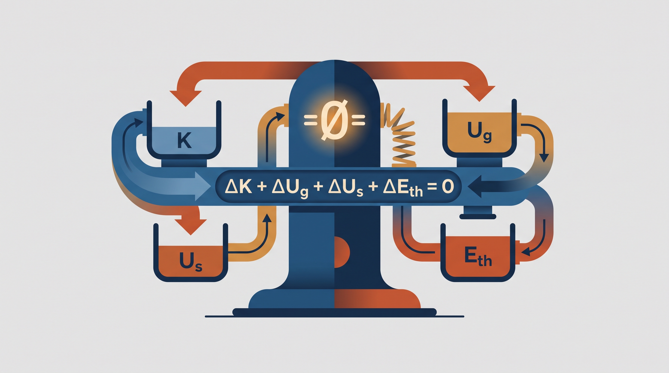
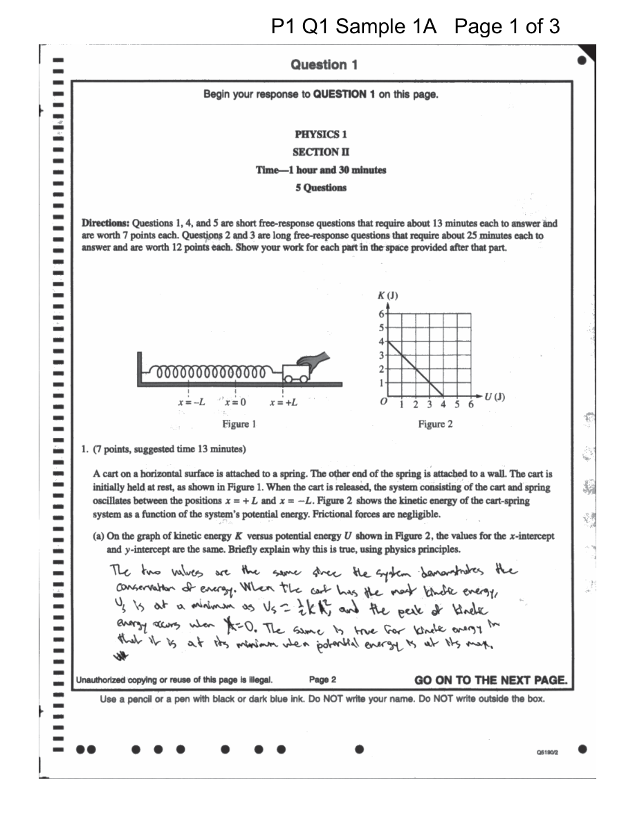
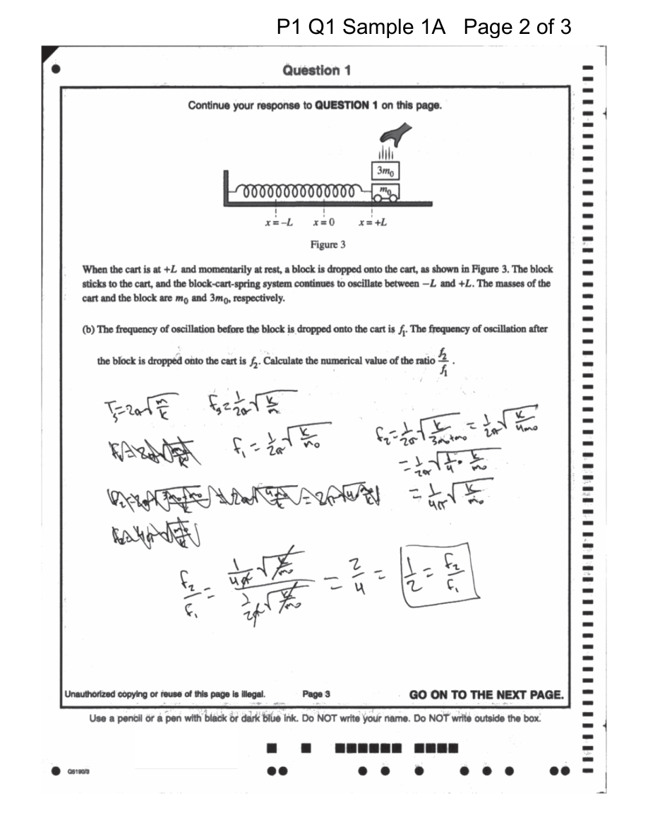
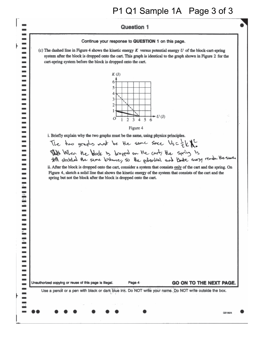
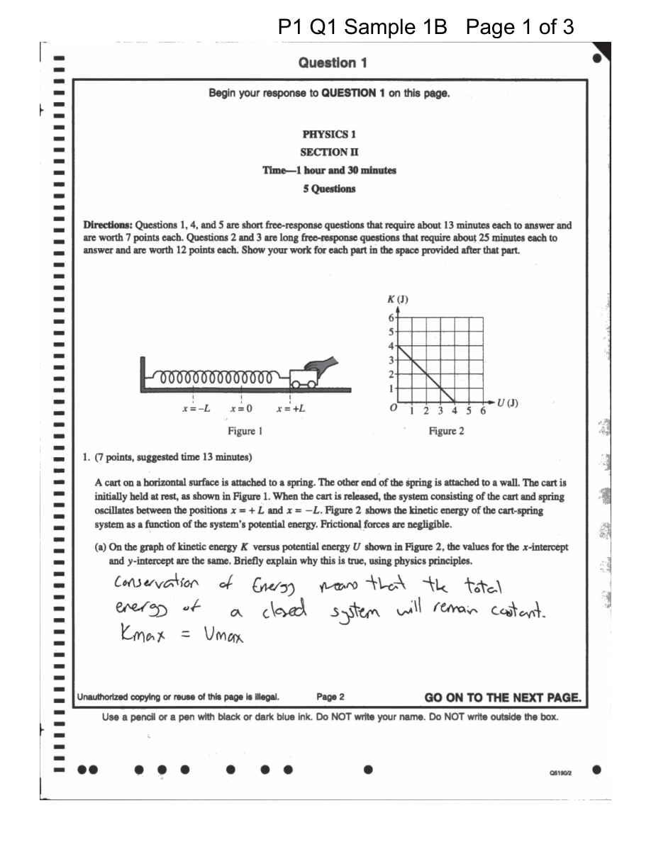
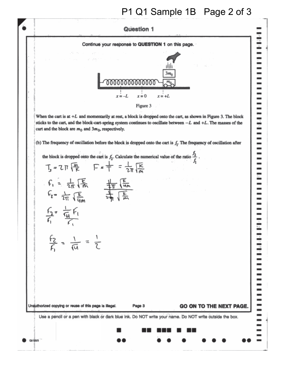
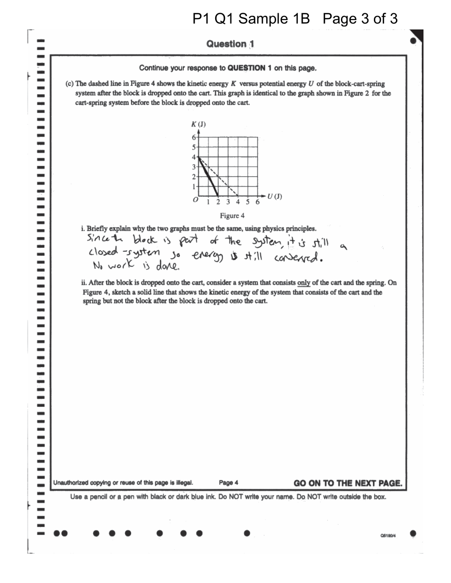
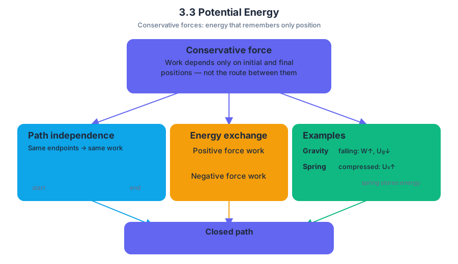
3.4 Conservation of Energy
Key concepts: Conservation of energy · Work–energy principle · Positive and negative work · Energy transformations caused by forces · Energy bar charts and system diagrams · Gravitational potential energy and kinetic energy · Rotational inertia and rotational kinetic energy · Symbolic derivation from known quantities · Energy conservation in ramps and vertical-loop motion · Conservation of momentum and kinetic energy in collisions
A cart can speed up, slow down, climb, dip, and loop without energy disappearing: energy changes form while the total energy of a chosen system remains constant.
3.4 Conservation of Energy
A cart can speed up, slow down, climb, dip, and loop without energy disappearing: energy changes form while the total energy of a chosen system remains constant. The central question is therefore not “Where did the energy go?” but “Which form of energy increased, and which form decreased?”
Conservation of energy: Energy cannot be created or destroyed. For an isolated system, the total energy remains constant even when energy is transformed between kinetic, potential, thermal, and other forms.
Work changes the energy of a system
Work is energy transferred to or from a system by a force acting through a displacement. The work–energy principle connects work directly to translational kinetic energy:
$$W_{\text{net}}=\Delta K=K_f-K_i$$
A force doing positive work transfers energy into the system’s kinetic energy or another internal form. A force doing negative work removes energy from the system or transfers it into another form.
For a constant force parallel to the displacement,
$$W=Fd$$
More generally,
$$W=Fd\cos\theta$$
where $\theta$ is the angle between the force and the displacement. A force perpendicular to the motion does zero work because $\cos 90^\circ=0$.
Consider a box sliding to the right. A pushing force pointing right does positive work and increases the box’s kinetic energy. Kinetic friction pointing left does negative work; if the box slows, its kinetic energy becomes thermal energy in the box and floor.
Misconception check — “Negative work means negative energy.”
Negative work is not a separate kind of energy. It describes energy transfer out of the system’s kinetic or mechanical energy, often into thermal energy.
The conservation-of-energy equation
Choose the system first. If the system includes the object, Earth, and any relevant spring, then gravitational or spring interactions can be represented as internal potential energy. For a system with no external energy transfer,
$$E_i=E_f$$
A common mechanical-energy form is
$$K_i+U_{g,i}+U_{s,i}=K_f+U_{g,f}+U_{s,f}$$
where
$$K=\frac{1}{2}mv^2,\qquad U_g=mgh,\qquad U_s=\frac{1}{2}kx^2$$
If friction or another external interaction transfers energy into the system as thermal energy, include that form explicitly rather than pretending mechanical energy is conserved.
Worked example: a cart and a vertical loop
A cart is released from rest at height $h_i$ above the bottom of a frictionless track. It rolls down a ramp and enters a vertical loop whose top is at height $2R$, where $R$ is the loop radius.
At release, $v_i=0$, so the initial energy is entirely gravitational:
$$E_i=mgh_i$$
At the top of the loop,
$$E_f=mg(2R)+\frac{1}{2}mv_{\text{top}}^2$$
Conservation of energy gives
$$mgh_i=mg(2R)+\frac{1}{2}mv_{\text{top}}^2$$
For the cart to remain in contact at the top, circular-motion dynamics requires a minimum speed satisfying
$$\frac{mv_{\text{top}}^2}{R}\geq mg$$
Thus,
$$v_{\text{top}}^2\geq gR$$
Substituting this minimum condition into the energy equation,
$$mgh_i\geq 2mgR+\frac{1}{2}mgR$$
so
$$h_i\geq \frac{5R}{2}$$
The release height must be greater than the top of the loop because the cart needs not only enough energy to reach that height, but also enough kinetic energy to maintain the required centripetal acceleration.
Energy bar charts and system diagrams
An energy bar chart displays the amount of each energy form at different moments. It is a representation, not a picture of the object. Begin with a zero-energy reference line, choose the system, and keep the vertical scale consistent.
For the cart released from rest and later moving at a lower height:
| State | $K$ | $U_g$ | Total |
|---|---|---|---|
| Release | $0$ | large | same |
| During descent | positive | smaller | same |
| Bottom of track | largest | near zero reference | same |
The exact bar heights must reflect the energy magnitudes. If the final gravitational-energy bar is half as large as the initial bar, the kinetic-energy bar must account for the missing amount. A chart that shows the correct energy types but inconsistent relative heights does not fully represent conservation.
Worked example: a rolling yo-yo
A yo-yo of mass $m$ and rotational inertia $I$ rolls down a ramp. If its string connects at radius $r$, and the yo-yo rolls without slipping, then
$$v=r\omega$$
The rotational inertia can be determined from the mass and connection radius when the yo-yo is modeled appropriately. For a simple rotating mass concentrated near radius $r$,
$$I=mr^2$$
If the yo-yo travels distance $d$ in time $t$ from rest with constant acceleration, then
$$d=\frac{1}{2}at^2$$
so
$$a=\frac{2d}{t^2},\qquad v^2=2ad=\frac{4d^2}{t^2}$$
Energy conservation relates the measured motion to the vertical drop $h$:
$$mgh=\frac{1}{2}mv^2+\frac{1}{2}I\omega^2$$
Using $\omega=v/r$,
$$mgh=\frac{1}{2}mv^2+\frac{1}{2}I\frac{v^2}{r^2}$$
This is a symbolic derivation: quantities are substituted in a logical sequence until the desired relationship appears.
Representations and AP Science Practices
Topic 3.4 explicitly develops these official science-practice skills:
- 1.A — Create diagrams, tables, charts, or schematics to represent physical situations. Draw the system boundary, identify energy forms, and construct scaled energy bars.
- 2.A — Derive a symbolic expression from known quantities by selecting and following a logical mathematical pathway. Start with conservation of energy, substitute relationships such as $v=r\omega$, and simplify step by step.
- 2.C — Compare physical quantities between two or more scenarios or at different times and locations in a single scenario. Compare speeds at different heights or determine which object has greater kinetic energy.
- 3.C — Justify or support a claim using evidence from experimental data, physical representations, or physical principles or laws. Use an energy chart, measured $d$ and $t$, or the conservation law to defend a conclusion.
Elastic collisions: energy and momentum together
In an ideal elastic collision, both momentum and kinetic energy are conserved. If object $A$ initially moves with speed $v_i$ and object $B$ is initially at rest, then
$$m_Av_i=m_Av_{f1}+m_Bv_{f2}$$
and
$$\frac{1}{2}m_Av_i^2=\frac{1}{2}m_Av_{f1}^2+\frac{1}{2}m_Bv_{f2}^2$$
Momentum conservation tracks the system’s motion; kinetic-energy conservation identifies the collision as elastic. Do not use kinetic-energy conservation for every collision: in an inelastic collision, some kinetic energy transforms into thermal energy, sound, or deformation.
Retrieval check
A sled moves down a rough incline. The sled’s gravitational potential energy decreases, its kinetic energy increases, and thermal energy also increases. Is the work done by friction positive or negative on the sled–Earth system, and which conservation equation would you write? The expected reasoning is that friction performs negative work on the mechanical motion while the complete system still satisfies $E_i=E_f$ when thermal energy is included.
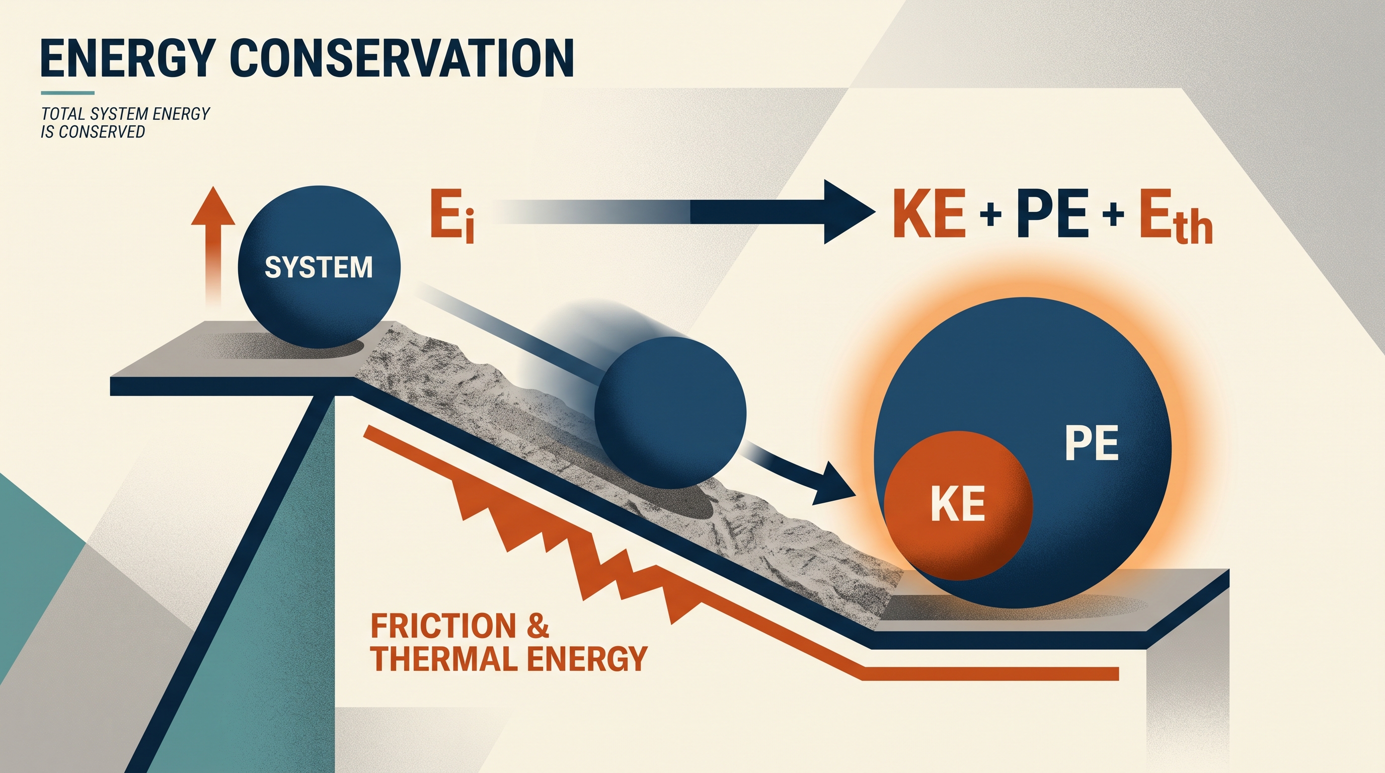
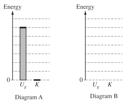
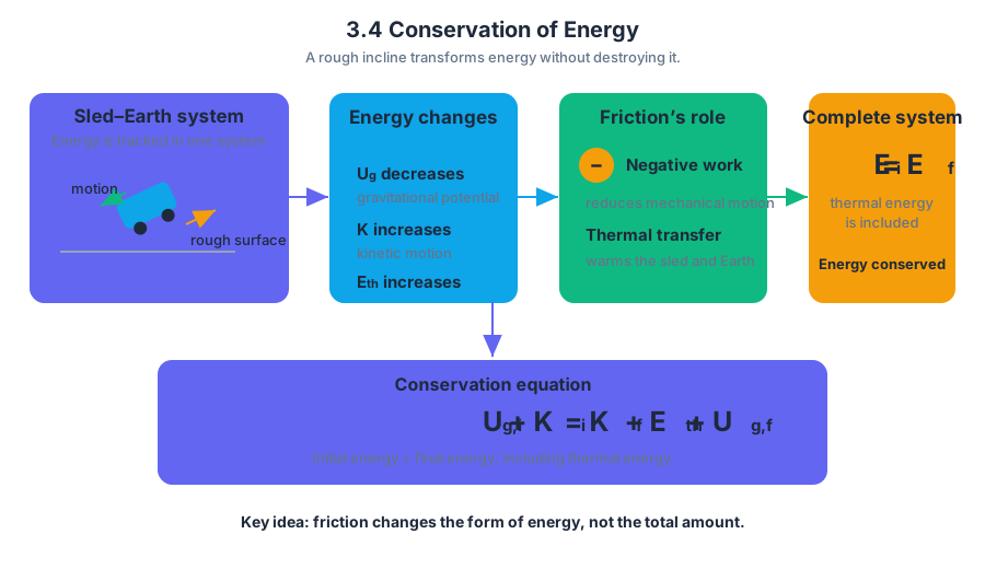
3.5 Power
Key concepts: Power
A machine that transfers the same amount of energy in less time is more powerful. Power measures the rate at which work is done, or equivalently the rate at which energy is transferred.
3.5 Power
A machine that transfers the same amount of energy in less time is more powerful. Power measures the rate at which work is done, or equivalently the rate at which energy is transferred.
Power is the amount of energy transferred per unit time.
The power formula is
$$ P=\frac{W}{\Delta t} $$
Here, $P$ is power, measured in watts; $W$ is work, or energy transferred, measured in joules; and $\Delta t$ is the time interval over which the transfer occurs, measured in seconds.
$$ 1\ \mathrm{W}=1\ \mathrm{J/s} $$
A watt is therefore not a separate kind of energy. It tells us how quickly energy is transferred. A $1000\ \mathrm{W}$ motor and a $100\ \mathrm{W}$ motor could each transfer $5000\ \mathrm{J}$, but the $1000\ \mathrm{W}$ motor does so in one-tenth the time.
Energy transferred versus power
Imagine two students carrying identical boxes through the same vertical distance. If both students do the same amount of work on their boxes, they transfer the same amount of energy. The student who finishes first produces the greater average power.
| Physical quantity | Meaning | Typical unit |
|---|---|---|
| Work, $W$ | Total energy transferred by a force | Joule, $\mathrm{J}$ |
| Time interval, $\Delta t$ | How long the transfer takes | Second, $\mathrm{s}$ |
| Power, $P$ | Rate of energy transfer | Watt, $\mathrm{W}$ |
The word average matters because the rate of transfer may vary. The formula gives the average power over the chosen interval. If a motor transfers $2400\ \mathrm{J}$ during an $8.0\ \mathrm{s}$ interval, its average power is
$$ P=\frac{W}{\Delta t} =\frac{2400\ \mathrm{J}}{8.0\ \mathrm{s}} =300\ \mathrm{W}. $$
This result means that, averaged over those $8.0\ \mathrm{s}$, the motor transfers energy at a rate of $300\ \mathrm{J/s}$. It does not mean that the motor transfers only $300\ \mathrm{J}$ total; the total transfer is still $2400\ \mathrm{J}$.
A contextual example: lifting a load
An elevator raises a $60\ \mathrm{kg}$ load vertically upward by $4.0\ \mathrm{m}$ in $8.0\ \mathrm{s}$. Ignore changes in kinetic energy and use $g=10\ \mathrm{m/s^2}$. What average power is required to increase the load’s gravitational potential energy?
The upward lift transfers energy against the gravitational force. The force needed for constant speed is approximately the load’s weight:
$$ F_g=mg =(60\ \mathrm{kg})(10\ \mathrm{m/s^2}) =600\ \mathrm{N}. $$
The work done during the lift is
$$ W=Fd =(600\ \mathrm{N})(4.0\ \mathrm{m}) =2400\ \mathrm{J}. $$
Now divide the energy transferred by the elapsed time:
$$ P=\frac{2400\ \mathrm{J}}{8.0\ \mathrm{s}} =300\ \mathrm{W}. $$
If the same load rises through the same distance in $4.0\ \mathrm{s}$, the work remains $2400\ \mathrm{J}$, but the power becomes
$$ P=\frac{2400\ \mathrm{J}}{4.0\ \mathrm{s}} =600\ \mathrm{W}. $$
The shorter time doubles the power. This proportional relationship is often the fastest way to reason: for a fixed amount of work, $P$ is inversely proportional to $\Delta t$.
Misconception check: “more power means more energy”
Misconception: A more powerful device always transfers more energy.
Correction: Power describes the rate of transfer, not the total transfer. A high-power device can transfer a fixed amount of energy quickly. A lower-power device can transfer that same amount more slowly. Total energy depends on both quantities:
$$ W=P\Delta t. $$
For example, a $500\ \mathrm{W}$ device operating for $6.0\ \mathrm{s}$ transfers
$$ W=(500\ \mathrm{W})(6.0\ \mathrm{s}) =3000\ \mathrm{J}. $$
A $1000\ \mathrm{W}$ device operating for only $3.0\ \mathrm{s}$ transfers the same $3000\ \mathrm{J}$. The devices have different powers but equal energy transfers.
Quick interpretation check
A student claims that completing $1200\ \mathrm{J}$ of work in $12\ \mathrm{s}$ is more powerful than completing $1800\ \mathrm{J}$ in $20\ \mathrm{s}$. Is the claim correct?
Calculate both rates:
$$ P_1=\frac{1200\ \mathrm{J}}{12\ \mathrm{s}}=100\ \mathrm{W}, \qquad P_2=\frac{1800\ \mathrm{J}}{20\ \mathrm{s}}=90\ \mathrm{W}. $$
Yes. The first process has the greater average power, even though it transfers less total energy. Always compare the ratio $\frac{W}{\Delta t}$ rather than comparing work alone.
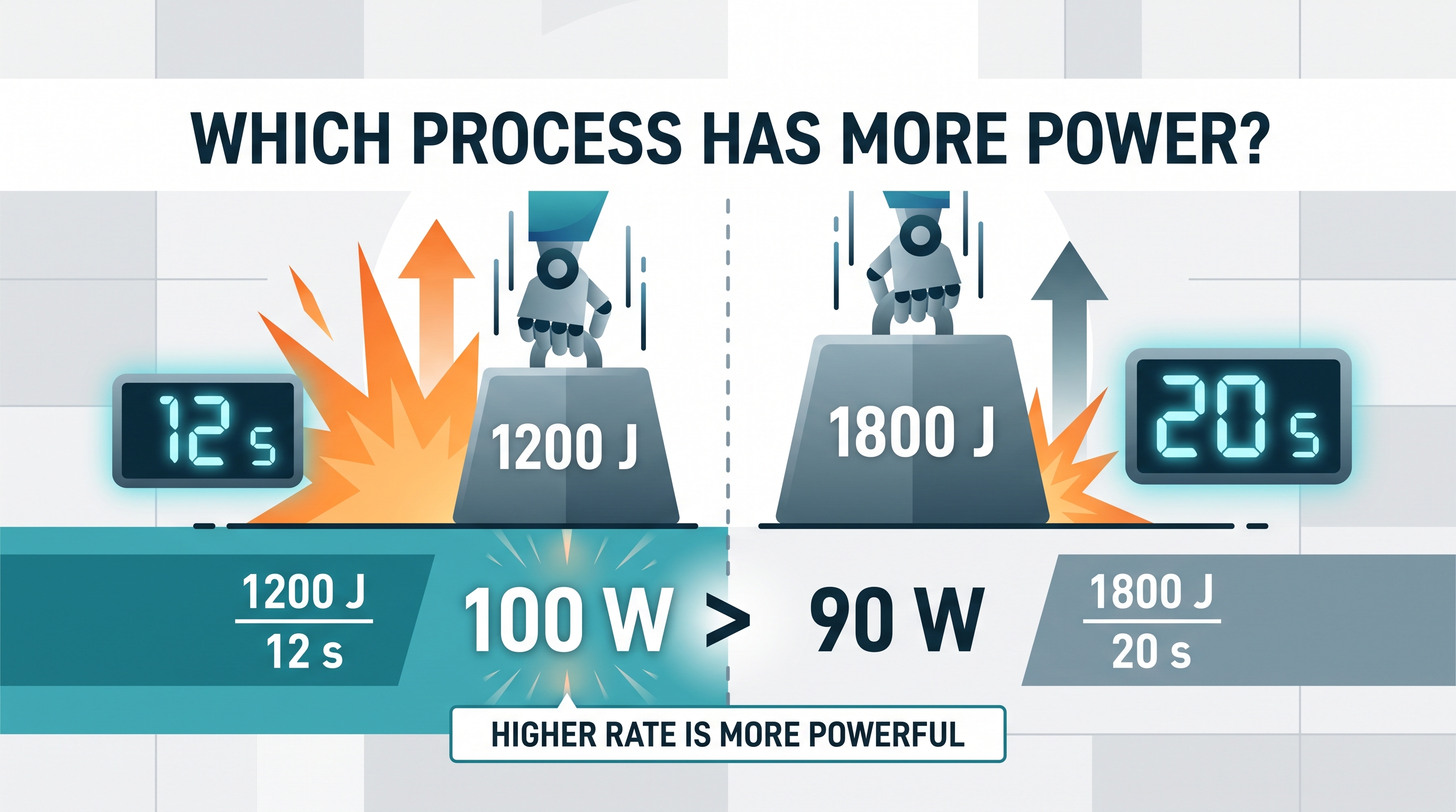
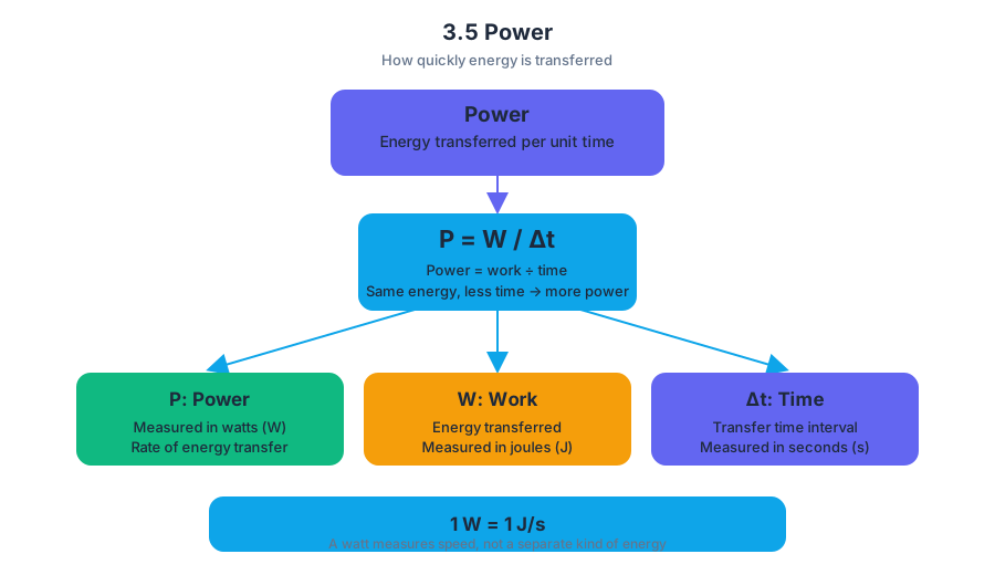
4.1 Linear Momentum
Key concepts: Linear momentum and impulse · Force–time graphs and momentum change · Velocity–time graphs and kinetic-energy change · Linear and angular quantities in rolling motion · Rolling while slipping versus pure rolling · Effect of friction on linear and angular speed · Translation between analogous linear and angular relationships · Using linear graphs to determine physical quantities · Spring-mass oscillations and period relationships
A rolling wheel can translate across the floor while rotating about its center, so its motion carries two linked descriptions: linear momentum for the motion of its center of mass and angular motion for its spin.
4.1 Linear Momentum
A rolling wheel can translate across the floor while rotating about its center, so its motion carries two linked descriptions: linear momentum for the motion of its center of mass and angular motion for its spin. The key is to connect these descriptions without assuming that they are literally the same quantity.
Linear momentum is the product of an object's mass and velocity:
$$\vec{p}=m\vec{v}$$
Momentum is a vector, so its direction is the direction of the velocity. Its SI unit is $\mathrm{kg\cdot m/s}$.
Momentum as “mass in motion”
A heavy cart and a light cart moving at the same velocity do not have the same momentum. Doubling the mass doubles the momentum; reversing the velocity reverses the momentum. A stationary object has zero linear momentum because $v=0$, even though it still has mass.
For a system of objects, total momentum is the vector sum of the individual momenta:
$$\vec{p}_{\text{system}}=\vec{p}_1+\vec{p}_2+\vec{p}_3+\cdots$$
The system boundary matters. Forces between objects inside the selected system can redistribute momentum within that system, but they do not change the system's total momentum by themselves. An external force can change the total momentum by exerting an impulse.
Force–time graphs reveal momentum change
The change in momentum is related to the net force acting over a time interval:
$$\Delta \vec{p}=\vec{F}_{\text{net}}\Delta t$$
For a force that varies with time, the change in momentum is estimated from the area under a force-versus-time graph:
$$\Delta \vec{p}\approx \text{area under the }F\text{-versus-}t\text{ graph}$$
For example, suppose a wheel experiences a horizontal force that rises linearly from $0$ to $12\ \mathrm{N}$ during $0.40\ \mathrm{s}$. The graph forms a triangle, so
$$\Delta p=\frac{1}{2}(0.40\ \mathrm{s})(12\ \mathrm{N})=2.4\ \mathrm{N\cdot s}$$
Because $\mathrm{N\cdot s}=\mathrm{kg\cdot m/s}$, the wheel's momentum changes by $2.4\ \mathrm{kg\cdot m/s}$ in the force's direction.
A graph must use a linear scale and clearly identified axes, including labels and units. A curved force graph is not averaged by simply using its highest value; its area must represent the accumulated effect of force over time.
Velocity–time graphs reveal kinetic-energy change
Momentum depends linearly on velocity, but translational kinetic energy depends on the square of velocity:
$$K=\frac{1}{2}mv^2$$
Thus, a velocity-versus-time graph can provide the initial and final speeds, which are then used to calculate the change in kinetic energy:
$$\Delta K=K_f-K_i=\frac{1}{2}m(v_f^2-v_i^2)$$
If a $2.0\ \mathrm{kg}$ cart changes speed from $3.0\ \mathrm{m/s}$ to $5.0\ \mathrm{m/s}$, then
$$\Delta K=\frac{1}{2}(2.0\ \mathrm{kg})\left[(5.0\ \mathrm{m/s})^2-(3.0\ \mathrm{m/s})^2\right]$$
$$\Delta K=16\ \mathrm{J}$$
The slope of a velocity-versus-time graph gives acceleration, while the values of velocity determine kinetic energy. The area under that graph instead represents displacement, not kinetic-energy change.
Linear and angular quantities in rolling
A rolling rigid body has a center-of-mass velocity $v$ and an angular velocity $\omega$. For pure rolling—rolling without slipping—the contact point is instantaneously at rest relative to the surface, and
$$v=R\omega$$
where $R$ is the wheel's radius. The analogous quantities form a useful translation:
| Linear quantity | Angular analogue |
|---|---|
| Position or displacement $x$ | Angular position $\theta$ |
| Velocity $v$ | Angular velocity $\omega$ |
| Acceleration $a$ | Angular acceleration $\alpha$ |
| Mass $m$ | Rotational inertia $I$ |
| Momentum $p=mv$ | Angular momentum $L=I\omega$ |
These are analogous relationships, not interchangeable ones. For example, $p=mv$ describes linear momentum, whereas $L=I\omega$ describes angular momentum. The symbols play parallel roles, but mass is not rotational inertia and velocity is not angular velocity.
A useful rolling investigation plots measured $v$ against measured $\omega$ for wheels of the same radius. From $v=R\omega$, the graph should be linear:
$$v=R\omega$$
If $v$ is on the vertical axis and $\omega$ is on the horizontal axis, the slope is
$$\text{slope}=\frac{\Delta v}{\Delta\omega}=R$$
For data with slope $0.080\ \mathrm{m}$, the wheel's radius is $R=0.080\ \mathrm{m}$. The graph therefore turns simultaneous linear and angular measurements into a physical measurement of radius. Clear axis labels and units are essential.
Rolling while slipping
Pure rolling is a special condition, not the definition of all rolling. During rolling while slipping, the wheel rotates and its center moves, but the contact point slides across the surface. Therefore $v$ and $\omega$ must be treated independently; the relation $v=R\omega$ does not apply during the slipping interval.
Kinetic friction acts at the contact region. Its effect is qualitative but predictable: it decreases the linear speed and changes the angular speed until the pure-rolling condition is reached. The exact time and distance of this transition are beyond the required model here, but the linked change in linear and angular quantities is essential.
Misconception check — “Friction always slows rotation.”
Friction opposes the relative slipping at the contact point, not automatically the wheel's angular velocity. Depending on whether the wheel spins too quickly or translates too quickly for pure rolling, friction can decrease or increase $\omega$ while also changing $v$.
A strong explanation identifies what is observed, states the expected relationship, and then connects the two logically: slipping means $v\neq R\omega$; kinetic friction changes the translational and rotational motion; the difference shrinks until $v=R\omega$.
Retrieval check
A wheel's graph of $v$ versus $\omega$ has slope $0.25\ \mathrm{m}$. What quantity does the slope represent? If the wheel is slipping, may you use $v=R\omega$ at that instant? Answer: the slope represents radius, $R=0.25\ \mathrm{m}$; no, the pure-rolling relation applies only when there is no slipping.

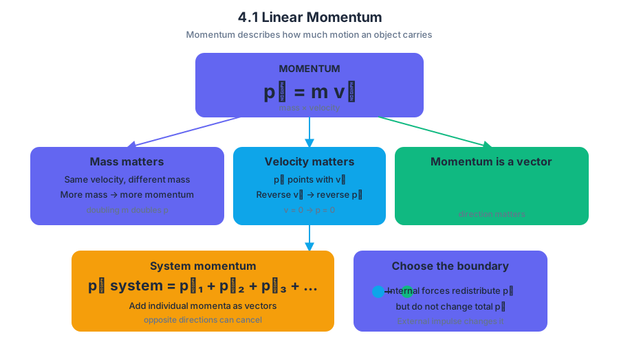
4.2 Change in Momentum and Impulse
Key concepts: Impulse · Change in linear momentum · Impulse-momentum theorem · Momentum bar charts · Effects of bouncing versus sticking collisions · Conservation of momentum in a selected system · Change in velocity and momentum during interactions · Transfer of kinetic energy in collisions · Experimental investigation of impulse and momentum
A dart that bounces from a cart can make the cart move faster than a dart that sticks to it—even when the dart has the same mass and incoming speed in both trials.
4.2 Change in Momentum and Impulse
A dart that bounces from a cart can make the cart move faster than a dart that sticks to it—even when the dart has the same mass and incoming speed in both trials. The decisive difference is not simply the force during impact; it is the dart’s change in momentum, which determines the impulse delivered to the cart.
Topic 4.2 — Change in Momentum and Impulse
Learning Objective: Use impulse and change in momentum to make claims about interactions.
Essential knowledge: The impulse delivered to an object or system equals its change in linear momentum.
Impulse is momentum transferred during an interaction
Impulse measures the effect of a force acting over a time interval. For a constant net force,
$$ \vec{J}=\vec{F}_{\text{net}}\Delta t $$
The impulse-momentum theorem connects that interaction to motion:
$$ \boxed{\vec{J}=\Delta \vec{p}=\vec{p}_f-\vec{p}_i} $$
Because linear momentum is $\vec{p}=m\vec{v}$, an object’s impulse can also be written as
$$ \vec{J}=m\vec{v}_f-m\vec{v}_i $$
Impulse is a vector, so direction matters. A large change in speed can produce a large impulse, but reversing direction is especially important: the initial and final velocity vectors point opposite ways, making the change in velocity—and therefore the change in momentum—larger.
Worked comparison: sticking versus bouncing
Suppose a dart has mass $m$ and initially moves right with velocity $+v$. Compare two interactions with a cart initially at rest.
| Interaction | Dart’s initial momentum | Dart’s final momentum | Dart’s momentum change |
|---|---|---|---|
| Dart sticks to cart | $+mv$ | approximately $0$ relative to the cart’s motion | $-mv$ |
| Dart bounces backward | $+mv$ | $-mv$ | $-2mv$ |
For the sticking case,
$$ \Delta p_{\text{dart}}=0-mv=-mv $$
For the bouncing case,
$$ \Delta p_{\text{dart}}=(-mv)-(+mv)=-2mv $$
The bounce gives the dart a change in momentum with twice the magnitude in this idealized comparison. By Newton’s third-law interaction, the cart receives an impulse equal in magnitude and opposite in direction to the dart’s impulse. Therefore, the bouncing dart delivers the greater impulse to the cart and produces the larger change in the cart’s momentum.
Misconception check — “The cart gets more impulse because the collision force is automatically larger.”
The safer reasoning is $\vec{J}=\Delta\vec{p}$. A force sensor may register a different force depending on collision time and springiness, but the total impulse is determined by the object’s momentum change. A short, intense force and a longer, gentler force can produce the same impulse.
Reading momentum bar charts
A momentum bar chart represents the momentum of each object before and after an interaction. Choose a positive direction first, then draw bars above the axis for positive momentum and below it for negative momentum. The change in a selected object’s bar is its impulse.
For the dart-cart system, the dart’s negative momentum change during a bounce corresponds to a positive momentum change for the cart. If the dart sticks, the dart does not reverse direction, so the cart receives less momentum. If the dart passes through the cart or stops and drops after impact, the same method applies: compare the dart’s initial and final momentum, then infer the cart’s impulse from the interaction.
Skill connection — Science Practice 1: Creating Representations. Translate the physical collision into velocity arrows, momentum bars, and a system diagram. The representation must show signs, not merely speeds.
Skill connection — Science Practice 2: Mathematical Routines. Use definitions and theoretical relationships such as $\vec{p}=m\vec{v}$ and $\vec{J}=\Delta\vec{p}$, maintaining a consistent sign convention.
Skill connection — Science Practice 3: Scientific Questioning and Argumentation. Make a claim—“the bounce gives the cart greater momentum”—and support it with the dart’s larger change in momentum. This is stronger than saying only that the bounce “looks more powerful.”
The arrow-and-pumpkin ranking
An arrow strikes a hanging pumpkin in three possible ways: it sticks, passes through, or bounces backward. The pumpkin’s initial momentum after the interaction is greatest when the arrow bounces and smallest when the arrow passes through, because the bounce produces the greatest change in the arrow’s momentum.
$$ \boxed{\theta_{\text{bounce}}>\theta_{\text{stick}}>\theta_{\text{pass}}} $$
After the collision, the pumpkin swings upward. Its kinetic energy is converted into gravitational potential energy,
$$ K \rightarrow U_g $$
so greater initial momentum gives the pumpkin greater initial speed and therefore a greater maximum height and swing angle. The ranking follows the impulse first, then the energy transformation after the collision.
Choosing a system
Momentum can remain constant when the chosen system has negligible net external impulse during the interaction. For example, selecting both the arrow and pumpkin includes the interaction forces inside the system; those forces are internal and cancel in the system’s total momentum accounting. Selecting only the pumpkin does not make its momentum constant, because the arrow exerts an external impulse on that smaller system.
Do not confuse this statement with conservation of kinetic energy. Momentum may be conserved for the selected system even while kinetic energy decreases because objects stick, deform, heat up, or make sound.
Retrieval check
A cart receives a dart that arrives moving right. In Case A the dart stops; in Case B it rebounds left with nearly its original speed. Which case gives the cart the greater impulse, and why? State the answer using one equation and one directional argument.
Answer: Case B. The dart’s momentum changes from approximately $+mv$ to $-mv$, so
$$ \Delta p_{\text{dart}}\approx -2mv $$
Its momentum-change magnitude is greater than in the stopping case, so the cart receives the greater opposite impulse.
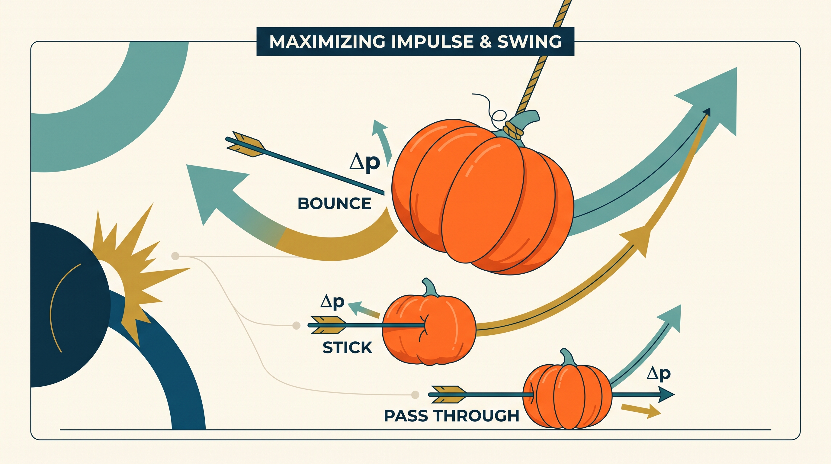
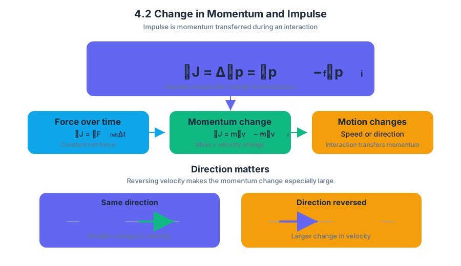
4.3 Conservation of Linear Momentum
Key concepts: Conservation of linear momentum for an isolated system · Perfectly inelastic collisions in which objects stick together · Momentum as the product of mass and velocity · Initial and final momentum of a multi-object system · Impulse–momentum theorem and its relation to Newton’s second law · Negligible external forces and friction in momentum-conservation problems · Using symbolic derivations to predict physical quantities · Qualitative reasoning and justification using physical principles and experimental evidence
Linear momentum is conserved when a system experiences negligible net external impulse: the system’s total momentum before an interaction equals its total momentum afterward. That single idea can predict the motion of colliding objects even when mechanical energy is transformed into sound, thermal energy, or…
4.3 Conservation of Linear Momentum
Linear momentum is conserved when a system experiences negligible net external impulse: the system’s total momentum before an interaction equals its total momentum afterward. That single idea can predict the motion of colliding objects even when mechanical energy is transformed into sound, thermal energy, or deformation.
4.3.A — Learning Objective: Describe the behavior of a system using conservation of linear momentum.
Momentum belongs to a system
Linear momentum is the product of an object’s mass and velocity:
$$\vec{p}=m\vec{v}$$
Because velocity is a vector, momentum has both magnitude and direction. A heavy, slowly moving object can have the same momentum as a light, rapidly moving object, provided the products $m\vec{v}$ are equal.
A collection of objects can be treated as one system. The system’s total momentum is the vector sum of the momenta of all its objects:
$$\vec{p}_{\text{system}}=\sum_i \vec{p}_i=\sum_i m_i\vec{v}_i$$
Its center-of-mass velocity is therefore
$$\vec{v}_{\text{cm}}=\frac{\sum \vec{p}_i}{\sum m_i} =\frac{\sum m_i\vec{v}_i}{\sum m_i}$$
If the net external force is zero, the center of mass moves at constant velocity. Internal forces may radically change the individual objects’ velocities, but they cannot change the total momentum of the complete system.
The conservation condition
The practical test is not whether any force acts. The test is whether the chosen system receives a significant net external impulse. If that impulse is negligible,
$$\vec{p}_i=\vec{p}_f$$
Equivalently, the total momentum change is zero:
$$\Delta \vec{p}_{\text{system}}=\vec{0}$$
A frictionless horizontal collision is a classic example. The blocks exert large forces on each other, but those forces are internal to the two-block system. The normal force from the surface and gravity act vertically, so they do not change the system’s horizontal momentum.
This is why system boundaries matter. For a block alone, the collision force from the other block is external, so the block’s momentum changes. For both blocks together, the collision forces are an internal action-reaction pair, so their impulses cancel in the total.
Perfectly inelastic collision: objects stick
A perfectly inelastic collision is a collision in which the objects stick together and share one final velocity. Consider Block 1, of mass $M_1$, moving right at speed $v_0$, striking stationary Block 2, of mass $M_2$, on a frictionless horizontal surface.
Before impact, the system’s horizontal momentum is
$$p_i=M_1v_0+M_2(0)$$
After the blocks stick, their combined mass is $M_1+M_2$, and both move with velocity $v_f$:
$$p_f=(M_1+M_2)v_f$$
Applying conservation of momentum,
$$M_1v_0=(M_1+M_2)v_f$$
so
$$\boxed{v_f=\frac{M_1v_0}{M_1+M_2}}$$
The final velocity points right because the initial system momentum points right.
Functional dependence and limiting reasoning
The equation predicts how changing $M_2$ affects $v_f$. Increasing $M_2$ increases the denominator while leaving the numerator unchanged, so the final speed decreases. If $M_1\gg M_2$, then $M_1+M_2\approx M_1$, giving
$$v_f\approx\frac{M_1v_0}{M_1}=v_0$$
Thus a much lighter stationary block barely slows the moving block. If instead $M_2$ is comparable to or much larger than $M_1$, the speed reduction is substantial. This qualitative estimate should agree with the symbolic equation.
Misconception check — “Sticking means momentum is lost.” Sticking means kinetic energy is generally not conserved; some energy becomes thermal energy, sound, or deformation. Momentum is still conserved whenever the system’s net external impulse is negligible.
A dropped block: conserve only the useful component
Suppose Block 2 is dropped vertically onto sliding Block 1 and sticks. Block 2 initially has zero horizontal velocity, even though it has downward velocity. Immediately after sticking, the combined blocks move horizontally:
$$M_1v_{1,i}+M_2v_{2,i,x}=(M_1+M_2)v_f$$
Since $v_{2,i,x}=0$,
$$v_f=\frac{M_1v_{1,i}}{M_1+M_2}$$
The horizontal speed decreases because the original horizontal momentum must now be shared by more mass. Vertical momentum is not conserved for the blocks alone because the surface exerts an external vertical impulse.
Momentum, impulse, and evidence
The impulse-momentum relationship follows directly from Newton’s second law for constant mass:
$$\vec{F}_{\text{net}}=\frac{\Delta\vec{p}}{\Delta t} =m\frac{\Delta\vec{v}}{\Delta t} =m\vec{a}$$
For a complete system, an external impulse changes total momentum:
$$\vec{J}{\text{ext}}=\Delta\vec{p}{\text{system}}$$
A momentum-versus-time graph has slope equal to the net external force. A force-versus-time graph has area equal to the external impulse. These representations help distinguish a real momentum change from an internal exchange.
The topic explicitly develops 1.B: Create quantitative graphs with appropriate scales and units, including plotting data; 2.A: Derive a symbolic expression from known quantities by selecting and following a logical mathematical pathway; 2.D: Predict new values or factors of change of physical quantities using functional dependence between variables; 3.A: Create experimental procedures that are appropriate for a given scientific question; and 3.C: Justify or support a claim using evidence from experimental data, physical representations, or physical principles or laws.
A strong experimental claim might combine a system diagram, measured velocities before and after a collision, a momentum calculation, and a graph. Agreement within measurement uncertainty supports conservation; noticeable external friction or an unaccounted force suggests that the system boundary or “negligible impulse” assumption must be reconsidered.
Retrieval check: Two carts stick together. Cart 1 has momentum $+6\ \mathrm{kg,m,s^{-1}}$ and Cart 2 is initially at rest. If their total mass is $3\ \mathrm{kg}$, what is their final velocity? Why is the answer not determined by conservation of mechanical energy?
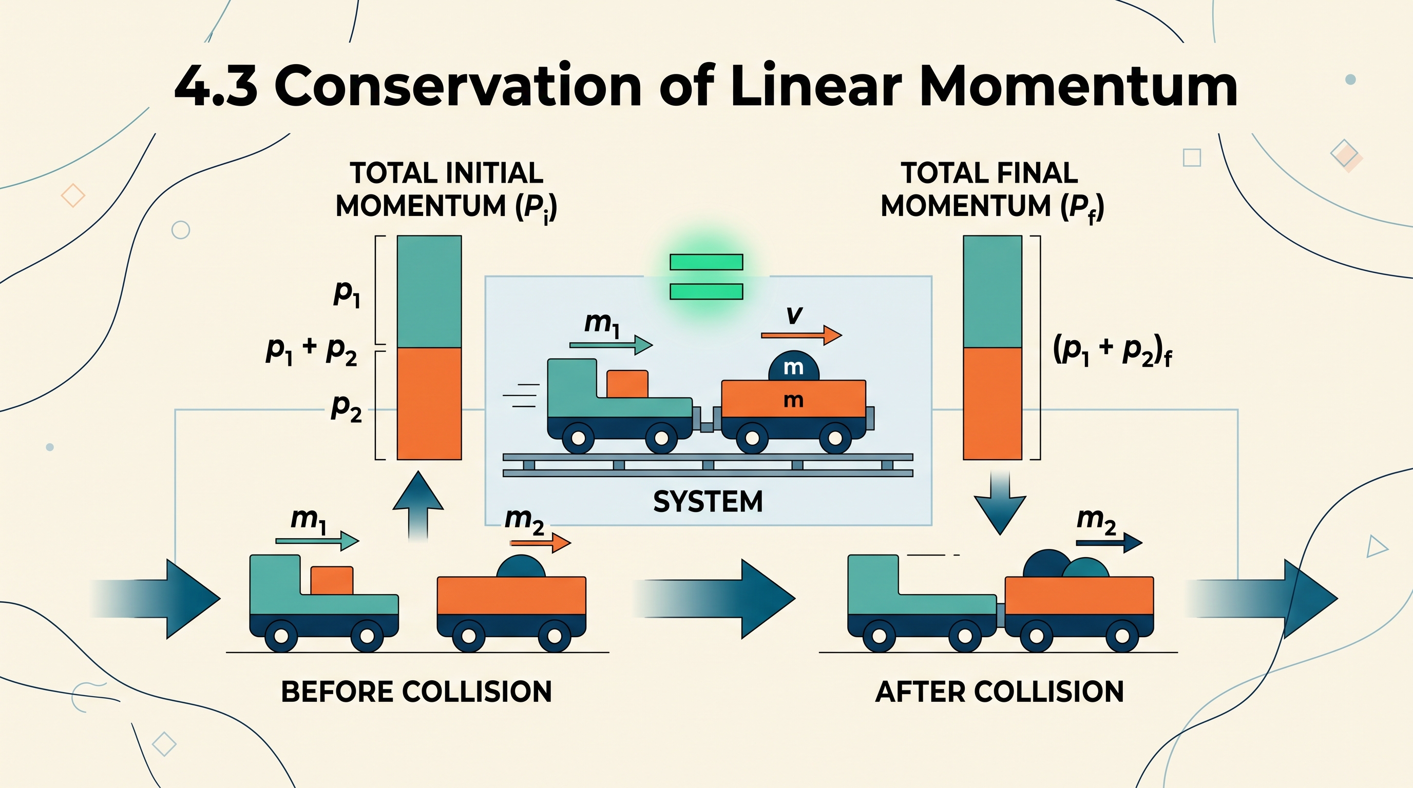
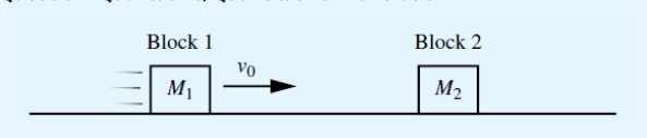
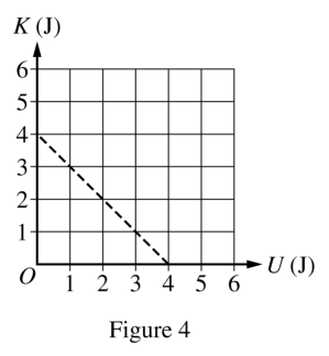
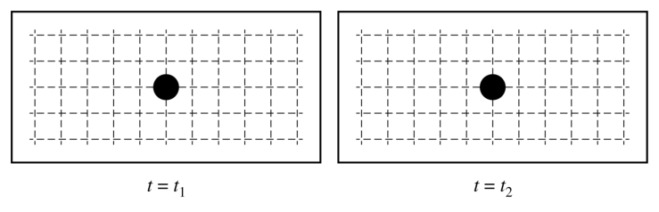
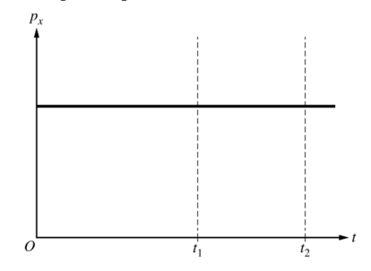

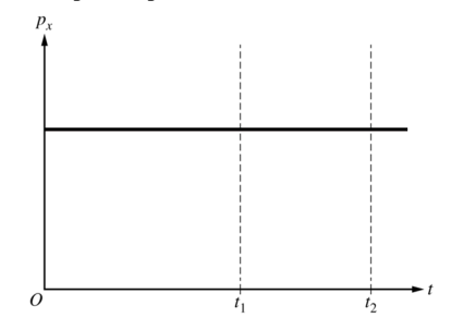
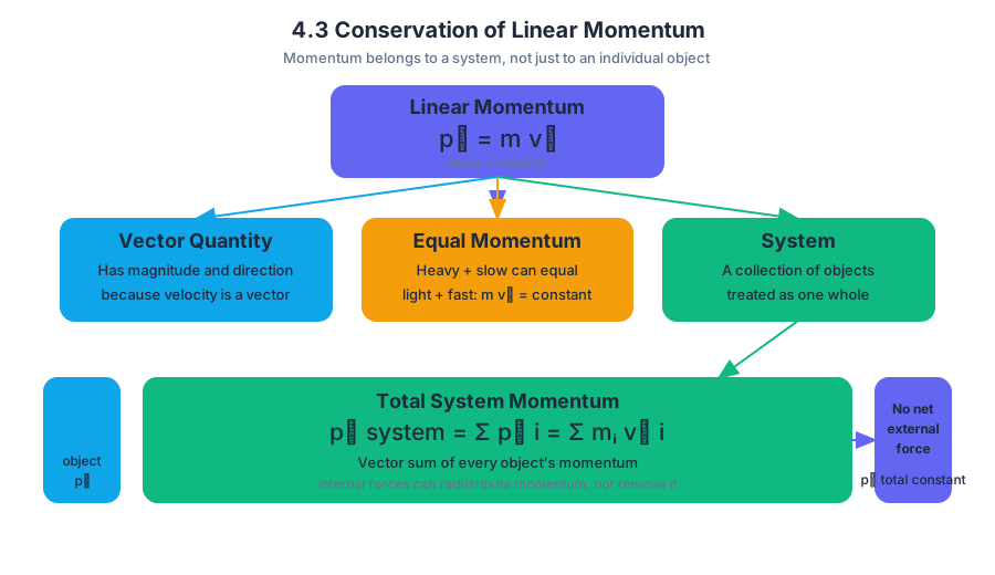
4.4 Elastic and Inelastic Collisions
Key concepts: Elastic collisions · Inelastic collisions · Conservation of momentum · Conservation of kinetic energy · Kinetic energy and speed · Position-versus-time graphs · Center of mass motion · Velocity as the slope of a position-versus-time graph · Collision-system modeling and external forces · Predicting changes using functional relationships
A collision can conserve the system’s total momentum while not conserving its kinetic energy. The key question is therefore not “Was momentum conserved?”—for an isolated two-object system, it is—but “What happened to the kinetic energy?”
4.4 Elastic and Inelastic Collisions
A collision can conserve the system’s total momentum while not conserving its kinetic energy. The key question is therefore not “Was momentum conserved?”—for an isolated two-object system, it is—but “What happened to the kinetic energy?”
Two collision classifications
Using the conservation-of-momentum result from Topic 4.3 for an isolated system, compare kinetic energy before and after the collision.
Elastic collision: Momentum and total kinetic energy are both conserved.
Inelastic collision: Momentum is conserved, but total kinetic energy is not conserved.
“Inelastic” does not mean that momentum disappears. Kinetic energy may be transformed into sound, thermal energy, deformation, or internal motion, while the vector total momentum of the two-object system remains unchanged. A collision in which objects stick together is a perfectly inelastic collision, but objects do not have to stick for a collision to be inelastic.
For two objects moving along one axis, apply
$$ m_Av_{A,i}+m_Bv_{B,i}=m_Av_{A,f}+m_Bv_{B,f}. $$
Then compare
$$ K_i=\frac{1}{2}m_Av_{A,i}^2+\frac{1}{2}m_Bv_{B,i}^2 $$
with
$$ K_f=\frac{1}{2}m_Av_{A,f}^2+\frac{1}{2}m_Bv_{B,f}^2. $$
The signs of velocity matter in the momentum equation; kinetic energy uses speed, so each squared velocity contributes positively.
Worked comparison: two carts
A $1.0\ \text{kg}$ cart moves at $3.0\ \text{m/s}$ toward a stationary $1.0\ \text{kg}$ cart. After the collision, the first cart stops and the second cart moves at $3.0\ \text{m/s}$.
Momentum:
$$ p_i=(1.0)(3.0)+(1.0)(0)=3.0\ \text{kg}\cdot\text{m/s} $$
$$ p_f=(1.0)(0)+(1.0)(3.0)=3.0\ \text{kg}\cdot\text{m/s}. $$
Kinetic energy:
$$ K_i=\frac{1}{2}(1.0)(3.0)^2=4.5\ \text{J} $$
$$ K_f=\frac{1}{2}(1.0)(3.0)^2=4.5\ \text{J}. $$
This collision is elastic.
Now suppose the same carts leave the collision with the first cart moving at $1.0\ \text{m/s}$ and the second at $2.0\ \text{m/s}$. Momentum is still
$$ p_f=(1.0)(1.0)+(1.0)(2.0)=3.0\ \text{kg}\cdot\text{m/s}, $$
but
$$ K_f=\frac{1}{2}(1.0)(1.0)^2+\frac{1}{2}(1.0)(2.0)^2=2.5\ \text{J}. $$
The missing $2.0\ \text{J}$ has been transformed into other forms of energy. This collision is inelastic.
Finding speed from kinetic energy
If an object starts from rest and gains kinetic energy, solve the kinetic-energy equation for its final speed:
$$ K=\frac{1}{2}mv^2 $$
$$ v=\sqrt{\frac{2K}{m}}. $$
For example, a stationary $2.0\ \text{kg}$ block gains $18\ \text{J}$ of kinetic energy. Its final speed is
$$ v=\sqrt{\frac{2(18\ \text{J})}{2.0\ \text{kg}}} =\sqrt{18}\ \text{m/s} \approx 4.2\ \text{m/s}. $$
The result is a speed, not a signed velocity. Direction requires additional information.
Misconception check: Doubling kinetic energy does not double speed. Because $K$ is proportional to $v^2$, speed changes with the square root of kinetic energy.
Reading collision motion on a position-versus-time graph
On a position-versus-time graph, the slope is velocity:
$$ v=\frac{\Delta x}{\Delta t}. $$
A constant velocity appears as a straight line. A positive slope means positive velocity; the object’s position itself may be positive, zero, or negative.
If Object A continues moving forward but slows down, its post-collision graph must have a positive slope that is less steep than its precollision slope. If Object B begins moving forward at constant speed, its post-collision graph is a straight line with a positive, nonzero slope.
The collision instant may appear as a corner where the slope changes. The vertical position at that instant does not jump unless the object undergoes an impossible instantaneous change in location; the slope changes because the velocity changes.
Center of mass through the collision
For two objects, the center-of-mass velocity is
$$ v_{\mathrm{CM}}=\frac{m_Av_A+m_Bv_B}{m_A+m_B}. $$
When no net external force acts on the two-object system, total momentum is constant, so $v_{\mathrm{CM}}$ remains constant before and after the collision.
Using the inelastic example with $m_A=m_B=1.0\ \text{kg}$, initial velocities $3.0\ \text{m/s}$ and $0$, and final velocities $1.0\ \text{m/s}$ and $2.0\ \text{m/s}$,
$$ v_{\mathrm{CM},i}=\frac{(1.0)(3.0)+(1.0)(0)}{2.0}=1.5\ \text{m/s} $$
and
$$ v_{\mathrm{CM},f}=\frac{(1.0)(1.0)+(1.0)(2.0)}{2.0}=1.5\ \text{m/s}. $$
Thus the center-of-mass position-versus-time graph has the same straight-line slope before and after the collision, even though the individual objects’ slopes change.
Retrieval check: A collision has conserved momentum, but the final kinetic energy is smaller than the initial kinetic energy. Is it elastic or inelastic? If Object A’s position graph changes from a steep positive slope to a less-steep positive slope, what happened to its velocity? Finally, if the system has no net external force, should the center-of-mass slope change? Explain each answer in one sentence.
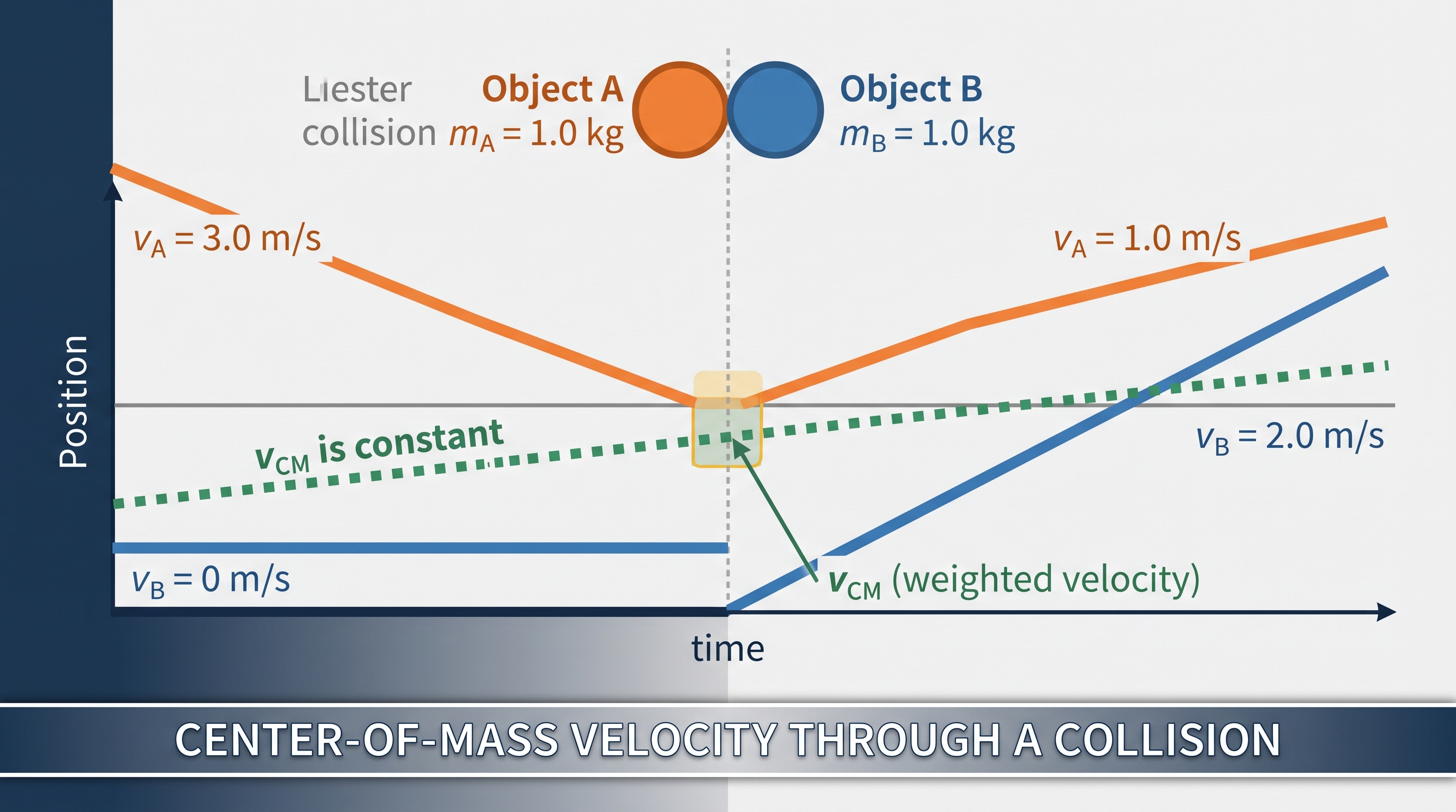
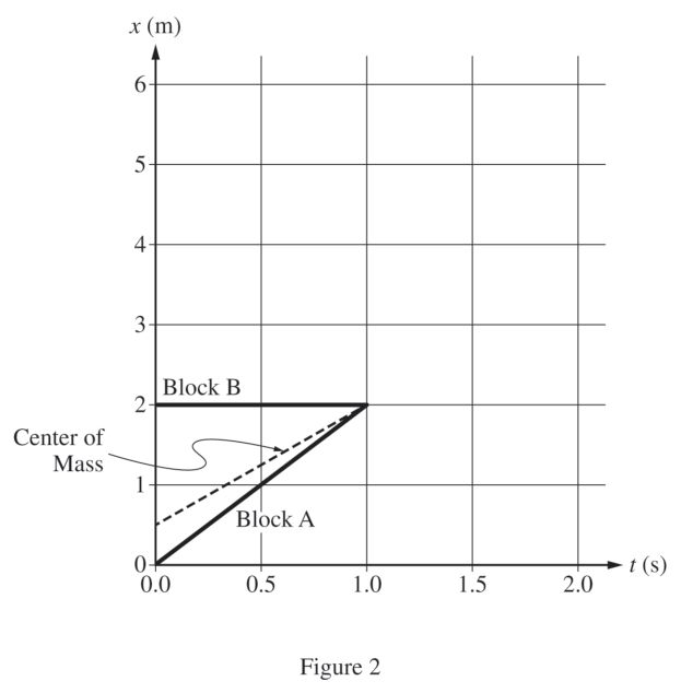
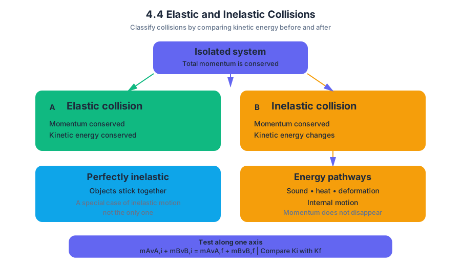
5.1 Rotational Kinematics
Key concepts: Angular speed as a function of time · Angular acceleration and the slope of an angular-speed–time graph · Rotation of a beam about a fixed hinge · Effect of cutting a string on rotational motion · Negligible-friction rotational dynamics · Qualitative interpretation of rotational graphs · Torque-dependent angular acceleration · Identifying and correcting discrepancies in prior work · Trigonometric dependence in tension equations
A beam released from a hinge does not generally spin with constant angular acceleration: gravity’s turning effect changes as the beam falls. That single fact determines the shape of its angular-speed graph.
5.1 Rotational Kinematics
A beam released from a hinge does not generally spin with constant angular acceleration: gravity’s turning effect changes as the beam falls. That single fact determines the shape of its angular-speed graph.
CED traceability: Topic 5.1 Rotational Kinematics; Learning Objective 5.A; Essential Knowledge 5.A.1 and 5.A.2. This topic applies Science Practice 1: Creating Representations, Science Practice 2: Mathematical Routines, and Science Practice 3: Scientific Questioning and Argumentation, especially the assessment skills Translation Between Representations and Qualitative/Quantitative Translation.
Angular position, angular speed, and angular acceleration
Angular position describes how far an object has rotated from a chosen reference direction. It is represented by $\theta$, measured in radians. Angular speed $\omega$ describes how rapidly the angular position changes:
$$ \omega = \frac{d\theta}{dt} $$
Angular speed is a scalar and is never negative. If direction matters, use angular velocity, which includes a sign or direction convention. Angular acceleration $\alpha$ describes how angular velocity changes with time:
$$ \alpha = \frac{d\omega}{dt} $$
The most important graph connection is:
The slope of an angular-speed-versus-time graph represents angular acceleration.
For a graph of $\omega$ against $t$,
$$ \text{slope}=\frac{\Delta \omega}{\Delta t}=\alpha $$
A horizontal line means $\alpha=0$; a rising line means positive angular acceleration; and a curve whose slope changes represents changing angular acceleration.
A hinged beam falling under gravity
Imagine a uniform beam held nearly horizontal by a string attached away from its hinge. When the string is cut, the beam rotates about the hinge with negligible friction. Gravity acts at the beam’s center of mass, so the gravitational torque is
$$ \tau_g = r_\perp mg $$
where $r_\perp$ is the perpendicular lever arm from the hinge to the line of action of the weight.
As the beam changes orientation, the lever arm changes. If the beam makes angle $\theta$ with the horizontal, one useful form is
$$ \tau_g = mg\left(\frac{L}{2}\right)\cos\theta $$
for a uniform beam of length $L$. The rotational form of Newton’s second law gives
$$ \tau_{\text{net}}=I\alpha $$
so
$$ \alpha=\frac{\tau_g}{I} \propto \cos\theta $$
The exact trigonometric form depends on how $\theta$ is defined, but the physical conclusion is unchanged: the angular acceleration changes as the beam falls because the gravitational torque depends on orientation.
At the instant after release, the beam is often positioned so that gravity produces a large torque. As the beam approaches vertical, the line of action of its weight passes closer to the hinge, reducing the torque. Therefore, the beam continues speeding up, but its speed increases more slowly.
Worked example: predicting the graph
A uniform beam starts from rest and falls from a nearly horizontal position toward vertical. Sketch $\omega$ as a function of time.
Step 1: Determine the initial value. The beam begins from rest, so
$$ \omega(0)=0 $$
The graph must begin at the origin.
Step 2: Determine the initial slope. Initially, the gravitational torque is nonzero, so $\alpha>0$. Because the slope of the $\omega$–$t$ graph is $\alpha$, the graph initially rises.
Step 3: Track the changing slope. As the beam approaches vertical, $\tau_g$ decreases. Thus $\alpha$ decreases, and the slope of the graph becomes smaller.
The correct qualitative graph rises from zero and gradually flattens:
This is not the same shape as the graph for a cart accelerating down a straight ramp. In the cart problem, the component of gravity along the ramp can remain constant, producing constant acceleration and a straight-line velocity graph. For the rotating beam, the torque changes with orientation, so the angular-speed graph is curved.
A discrepancy worth catching
A common first attempt is a straight line sloping downward from a positive angular speed. That graph contains two errors: the beam begins from rest, and gravity makes its angular speed increase rather than decrease.
A graph is a physical claim. Its starting value, direction, slope, and curvature must all agree with the motion.
If an earlier graph or calculation predicts decreasing $\omega$ while the beam is falling, identify the discrepancy explicitly: the prediction contradicts the direction of the gravitational torque. If it predicts constant $\alpha$, it has treated the torque as constant even though the lever arm changes.
Connected reasoning: tension and trigonometry
In a related static or constrained-rotation calculation, balancing torques can produce a tension such as
$$ F_T=\frac{mg,r_g}{r_T\sin\phi} $$
where $\phi$ is the angle between the string and the beam. The trigonometric factor appears because only the perpendicular component of tension produces torque. As $\sin\phi$ becomes small, the required tension can become large; using the entire tension as a turning force is a modeling error.
Misconception check
Misconception: “Constant gravity means constant angular acceleration.” Gravity’s magnitude is approximately constant near Earth’s surface, but torque depends on the perpendicular lever arm. Since that lever arm changes during rotation, angular acceleration need not remain constant.
Retrieval check: A rotating object’s $\omega$–$t$ graph is increasing but concave down. What does that say about $\alpha$? The angular acceleration is positive but decreasing: $\omega$ is still increasing, while the slope of the graph is becoming smaller.


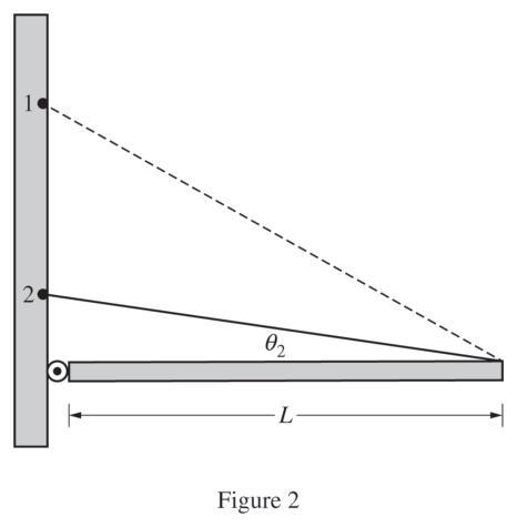
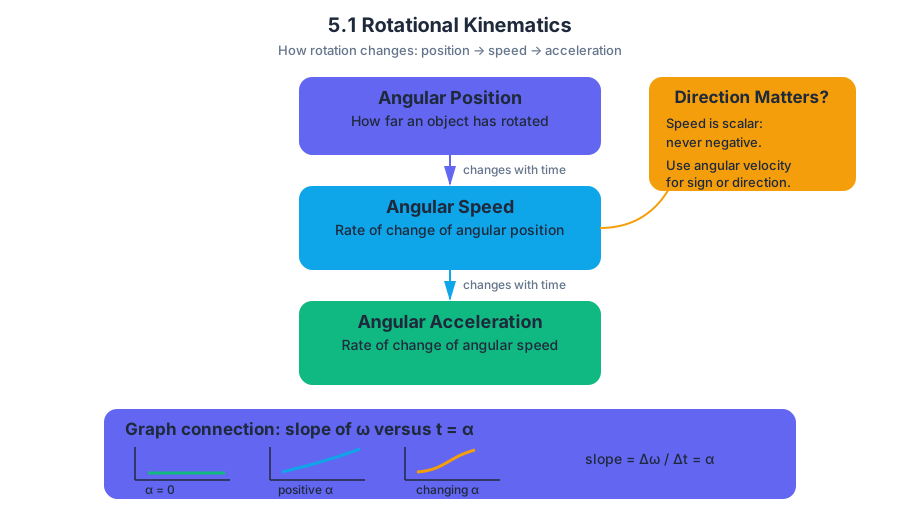
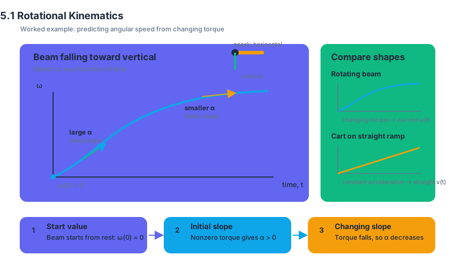
5.2 Connecting Linear and Rotational Motion
Key concepts: Connecting linear and rotational motion · Relationship between linear and angular quantities for a rotating rigid body · Tangential velocity and angular velocity · Tangential acceleration and angular acceleration · Rigid-body rotation about a fixed axis · Rolling motion without slipping · Applying laws, definitions, and theoretical relationships to make claims · Calculating unknown quantities with units from known quantities · Creating quantitative graphs with appropriate scales and units · Rolling while slipping is beyond the scope of AP Physics 1
A rotating wheel can have one angular velocity but many different linear velocities: points farther from the axle travel faster because they sweep through the same angle along larger circular arcs.
5.2 Connecting Linear and Rotational Motion
A rotating wheel can have one angular velocity but many different linear velocities: points farther from the axle travel faster because they sweep through the same angle along larger circular arcs. The key question is: How does an angular description of motion become a linear description?
The geometry of a rotating rigid body
A rigid body is an object whose shape does not change as it moves. When it rotates about a fixed axis, every point turns through the same angular displacement $\Delta\theta$, but points at different distances $r$ from the axis travel different linear distances.
For a point at radius $r$, the arc length traveled is
$$ \Delta s = r\Delta\theta $$
where $\Delta\theta$ must be measured in radians. One complete revolution is $2\pi$ radians, so a point on the rim of radius $R$ travels $2\pi R$ during one revolution.
The equation explains why the axle and rim of a rotating wheel do not have the same linear speed. They share the same $\Delta\theta$, but the rim has a greater $r$.
From angular velocity to tangential velocity
Dividing $\Delta s=r\Delta\theta$ by the time interval $\Delta t$ produces the relationship between linear and angular velocity:
$$ v = r\omega $$
Here, $\omega$ is angular velocity and $v$ is the tangential velocity, the instantaneous linear velocity directed tangent to the circular path. The angular velocity is the same for every point on a rigid body rotating about one fixed axis, but $v$ increases directly with $r$.
For example, a disk rotates with $\omega=4.0\ \mathrm{rad/s}$. A point $0.10\ \mathrm{m}$ from the axis has
$$ v=(0.10\ \mathrm{m})(4.0\ \mathrm{rad/s}) =0.40\ \mathrm{m/s} $$
A point at $r=0.30\ \mathrm{m}$ has
$$ v=(0.30\ \mathrm{m})(4.0\ \mathrm{rad/s}) =1.2\ \mathrm{m/s} $$
Both points complete each revolution together, but the outer point covers three times as much distance in the same time.
Tangential acceleration
When the angular velocity changes, the tangential speed changes. Differentiating $v=r\omega$ with respect to time for a fixed radius gives
$$ a_t=r\alpha $$
where $a_t$ is the tangential component of acceleration and $\alpha$ is angular acceleration. This component changes the magnitude of the velocity, while the inward, or radial, component changes its direction.
A point twice as far from the axis has twice the tangential acceleration when the entire rigid body has the same $\alpha$. For $\alpha=3.0\ \mathrm{rad/s^2}$ and $r=0.25\ \mathrm{m}$,
$$ a_t=(0.25\ \mathrm{m})(3.0\ \mathrm{rad/s^2}) =0.75\ \mathrm{m/s^2} $$
The radius must be fixed for this direct conversion. If a point moves inward or outward, additional reasoning is required.
Connecting quantities across locations
For two points on the same rotating rigid body,
$$ \frac{v_1}{v_2}=\frac{r_1}{r_2} \qquad\text{and}\qquad \frac{a_{t1}}{a_{t2}}=\frac{r_1}{r_2} $$
provided both points share the same angular velocity or angular acceleration, respectively. This is a useful comparison strategy: do not calculate every quantity from scratch when proportional reasoning is enough.
Misconception check — “Every point on a wheel has the same velocity.” Every point has the same angular velocity, but not the same velocity vector. The speed depends on $r$, and the direction is tangent to the circle, so the direction also changes from point to point.
Rolling without slipping
A wheel rolls without slipping when the point of contact with the surface is instantaneously at rest relative to that surface. The center of mass moves forward while the wheel rotates, and the two motions are linked by
$$ v_{\mathrm{cm}}=R\omega $$
For changing motion, the corresponding relation is
$$ a_{\mathrm{cm}}=R\alpha $$
where $R$ is the wheel radius.
A bicycle wheel with $R=0.35\ \mathrm{m}$ rotating at $\omega=8.0\ \mathrm{rad/s}$ has center-of-mass speed
$$ v_{\mathrm{cm}}=(0.35\ \mathrm{m})(8.0\ \mathrm{rad/s}) =2.8\ \mathrm{m/s} $$
If the wheel slides while rotating, these equations no longer directly connect its center-of-mass motion to its rotation.
Key insight: In fixed-axis rotation, angular quantities describe the whole rigid body; linear quantities depend on the point’s distance from the axis.
AP skills in action
This topic explicitly develops 1.C: Create qualitative sketches of graphs that represent features of a model or the behavior of a physical system by recognizing that $v$ versus $r$ is a straight line through the origin with slope $\omega$.
It develops 2.A: Derive a symbolic expression from known quantities by selecting and following a logical mathematical pathway through $\Delta s=r\Delta\theta$, $v=r\omega$, and $a_t=r\alpha$. It develops 2.C: Compare physical quantities between two or more scenarios or at different times and locations in a single scenario through radius-based ratios, and 3.B: Apply an appropriate law, definition, theoretical relationship, or model to make a claim when using the rolling condition or any linear-angular relationship.
Retrieval check: A disk has constant $\omega$. If the radius changes from $r$ to $3r$, what happens to tangential speed? What happens to angular speed? The answer is $v\rightarrow3v$, while $\omega$ remains unchanged for the rigid disk.
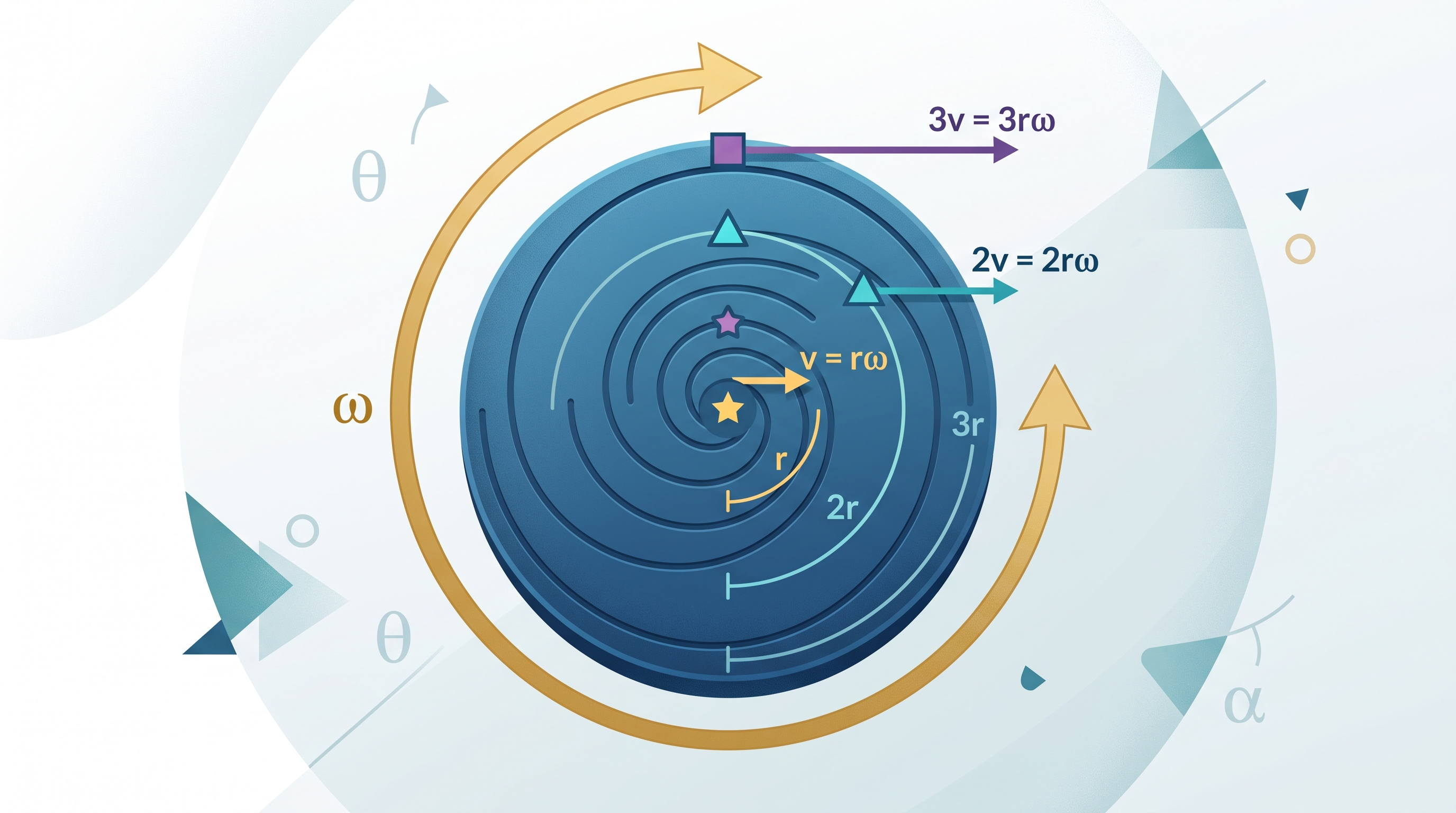
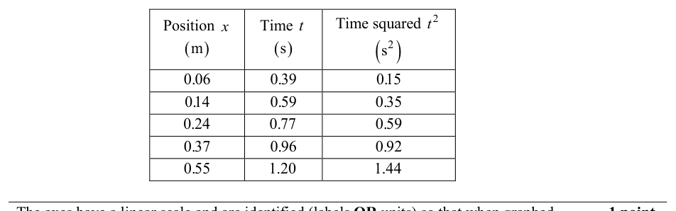
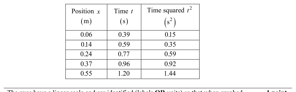
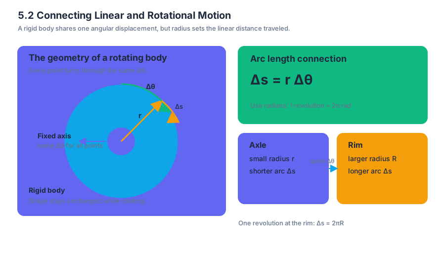
5.3 Torque
Key concepts: Torque · Angle · Radial distance or lever arm (r) · Density · Cosine relationship
A force can make an object accelerate without making it rotate, depending on where and how the force acts. Pushing a door near its hinges is difficult; pushing at the handle is effective because the turning effect depends on both the force and its distance from the axis.
5.3 Torque
A force can make an object accelerate without making it rotate, depending on where and how the force acts. Pushing a door near its hinges is difficult; pushing at the handle is effective because the turning effect depends on both the force and its distance from the axis.
The turning effect of a force
Torque, represented by the symbol $\tau$, measures how strongly a force tends to rotate an object about a chosen axis. Its unit is the newton-meter, written $\text{N}\cdot\text{m}$.
Torque is the rotational counterpart of a force’s ability to produce linear acceleration.
The torque magnitude depends on three ingredients:
- the force magnitude, $F$;
- the radial distance, or lever arm, $r$, from the axis to the point where the force acts;
- the angle between the radial direction and the force direction.
A form commonly shown on the AP Physics 1 reference sheet is
$$ \tau = rF\cos(\text{angle}). $$
In this cosine form, the angle is measured between the applied force and the direction perpendicular to the radius. If instead the angle is measured between $\vec r$ and $\vec F$, the equivalent relation is
$$ \tau = rF\sin\theta. $$
The two expressions describe the same physics; they use complementary angle conventions.
Why the lever arm matters
The lever arm is the distance $r$ from the rotation axis to the point of application of the force. Increasing $r$ increases torque when the force and angle remain unchanged:
$$ \tau \propto r. $$
Doubling the distance from the hinge doubles the torque. This is why a long wrench loosens a bolt more easily than a short wrench when the same force is applied.
The angle determines how much of the force produces rotation. A force directed perpendicular to the radius gives the greatest torque. A force directed along the radius gives no torque because its line of action points toward or away from the axis rather than around it.
Worked example: opening a hatch
A student pushes a hatch with a force of $40\ \text{N}$. The force is applied $0.75\ \text{m}$ from the hinge, and the angle measured in the cosine form is $20^\circ$ from the perpendicular direction. The torque magnitude is
$$ \tau = rF\cos(20^\circ). $$
Substitute the values:
$$ \tau = (0.75\ \text{m})(40\ \text{N})\cos(20^\circ) $$
$$ \tau \approx (30)(0.940) $$
$$ \boxed{\tau \approx 28\ \text{N}\cdot\text{m}}. $$
The force produces a counterclockwise or clockwise torque depending on which side of the hinge it is applied and which direction it pushes. A complete free-body or rotational diagram should show the axis, the radius vector, the force vector, and the angle convention.
Misconception check — “A larger force always means a larger torque.” Not necessarily. A large force applied directly toward the axis can produce $\tau=0$, while a smaller force applied far from the axis and perpendicular to the radius can produce substantial torque.
Density and physical quantities
Density is a quantity describing how much mass is contained in a given volume:
$$ \rho = \frac{m}{V}. $$
Its SI unit is $\text{kg}/\text{m}^3$. Density is not a factor in the torque expression itself. However, it can be used to determine an object’s mass from its volume when mass is needed in a larger rotational-dynamics problem. The constants and conversion information associated with torque may therefore list density alongside quantities such as angle, torque, and angular speed, even though density does not appear in $\tau=rF\cos(\text{angle})$.
AP reasoning in action
This topic primarily uses Science Practice 1: Creating Representations, especially a diagram that identifies the rotation axis, radius, force, and angle. It also uses Science Practice 2: Mathematical Routines when students select the correct trigonometric form, substitute values, track units, and reason proportionally. Science Practice 3: Scientific Questioning and Argumentation appears when students justify why one force placement or direction produces more torque than another.
A strong representation should make the rotational cause visible rather than merely listing numbers. Before calculating, ask: What is the axis? How far from it does the force act? Which component of the force is perpendicular to the radius?
Retrieval check
A force of $25\ \text{N}$ acts $0.40\ \text{m}$ from an axis directly perpendicular to the radius. What is the torque magnitude?
$$ \tau=(0.40\ \text{m})(25\ \text{N})\cos(0^\circ) =\boxed{10\ \text{N}\cdot\text{m}}. $$
If the same force points directly along the radius, the torque is $\boxed{0\ \text{N}\cdot\text{m}}$, regardless of the value of $F$ or $r$.
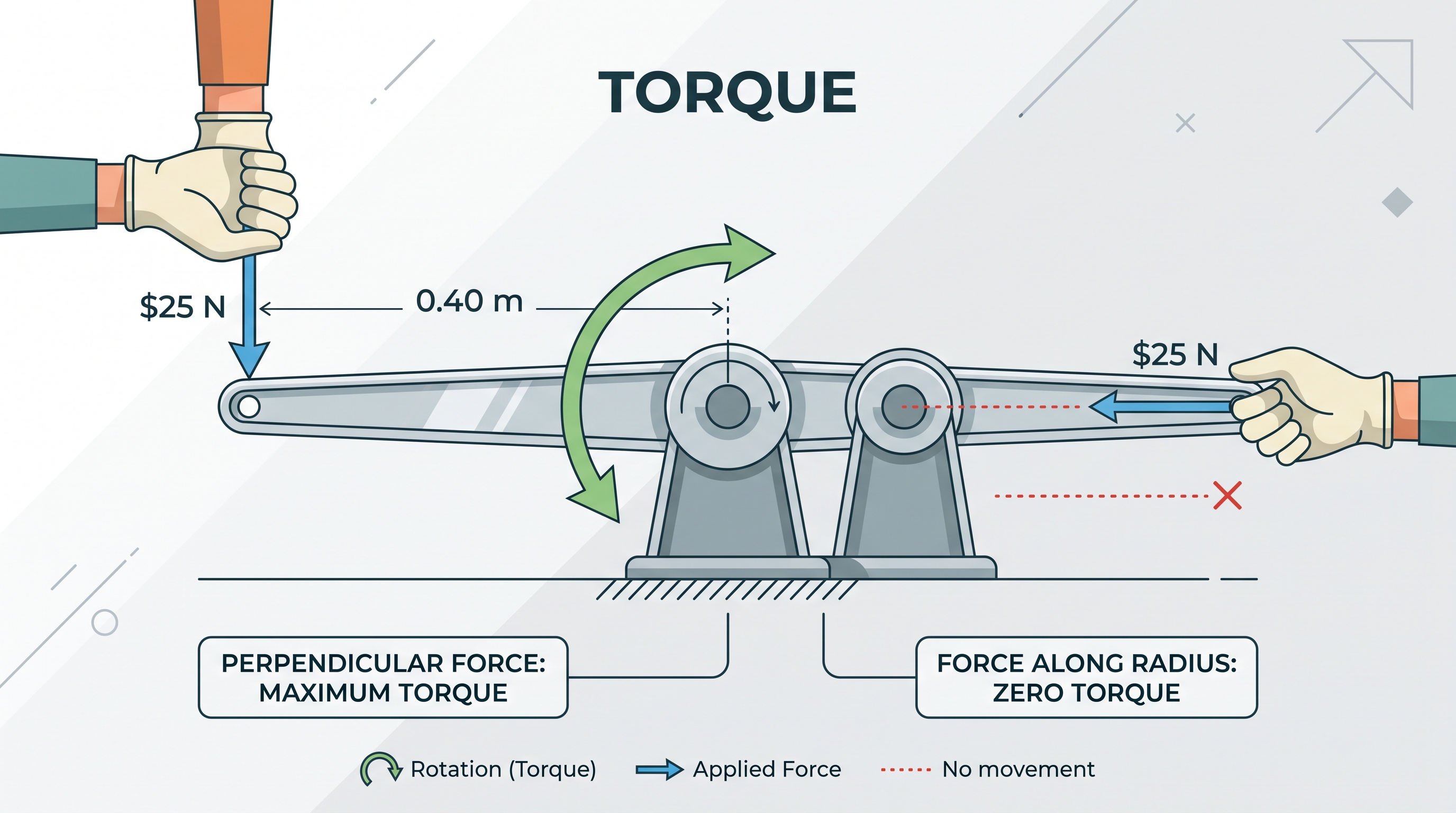
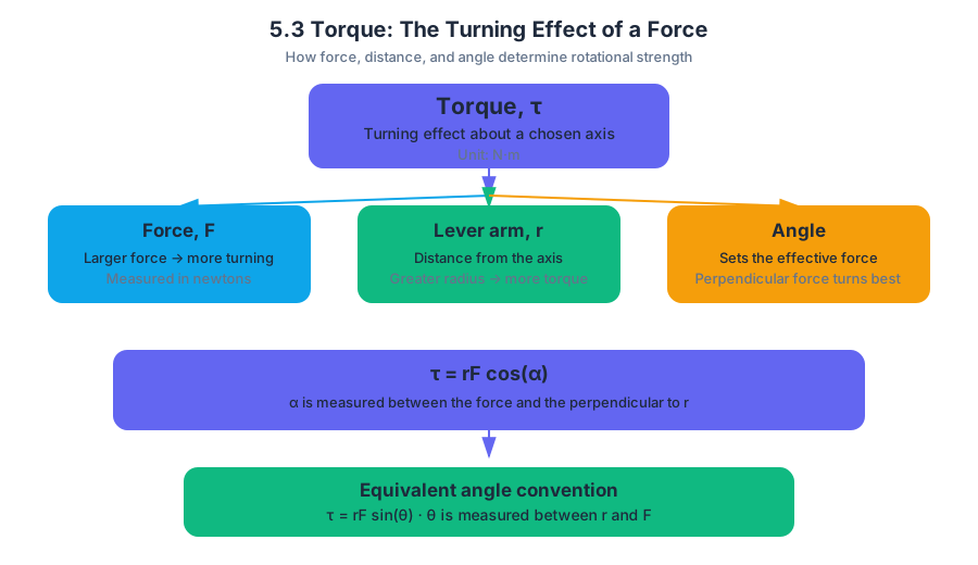
5.4 Rotational Inertia
Key concepts: Rotational inertia · Moment of inertia of disks and hoops · Dependence of rotational inertia on mass and radius · Torque produced by a tangential force · Relationship between torque, rotational inertia, and angular acceleration · Angular momentum and equal torque applied for equal time · Rotational kinetic energy and work · Rolling objects and acceleration down an incline · Experimental effects of wheel rotational inertia on measured acceleration and g_exp · Using physical models to explain observable rotational motion
A wheel does not resist changes in rotation merely because it has mass; it resists them according to where its mass is located relative to the axis.
5.4 Rotational Inertia
A wheel does not resist changes in rotation merely because it has mass; it resists them according to where its mass is located relative to the axis. That rotational resistance is called rotational inertia, or moment of inertia, and is represented by $I$.
Rotational inertia measures how difficult it is to change an object’s angular motion. More mass, or mass located farther from the rotation axis, generally means greater $I$.
Mass distribution determines rotational inertia
Imagine releasing a solid disk and a thin hoop from the same incline. Both have the same mass $M$ and radius $R$, but the hoop places nearly all of its mass at distance $R$ from the axis, while the disk distributes mass from the center outward. The hoop therefore has greater rotational inertia.
For a disk or pulley modeled as a uniform disk,
$$ I_{\text{disk}}=\frac{1}{2}MR^2 $$
For a thin hoop,
$$ I_{\text{hoop}}=MR^2 $$
Thus, for equal $M$ and $R$,
$$ I_{\text{hoop}}=2I_{\text{disk}} $$
The hoop is harder to spin up because more of its mass lies far from the axis. This is why cans with different contents can reach the bottom of an incline at different times even when their diameters are identical.
The rotational motion model
A complete model identifies the object’s mass $M$, radius $R$, applied tangential force or tension $F_T$, torque $\tau$, rotational inertia $I$, and angular acceleration $\alpha$.
A tension applied tangent to a disk acts at right angles to the radius. Therefore, using the torque relationship from the preceding topic,
$$ \tau=RF_T $$
The rotational form of Newton’s second law connects torque to angular acceleration:
$$ \alpha=\frac{\tau}{I} $$
This equation contains the central idea: the same torque produces less angular acceleration when rotational inertia is larger.
Worked example: disk versus hoop
A disk and a hoop each have mass $M=0.40\ \text{kg}$ and radius $R=0.10\ \text{m}$. A tangential force $F_T=0.20\ \text{N}$ acts on each for $0.50\ \text{s}$.
For the disk,
$$ I_d=\frac{1}{2}(0.40)(0.10)^2=0.0020\ \text{kg}\cdot\text{m}^2 $$
For the hoop,
$$ I_h=(0.40)(0.10)^2=0.0040\ \text{kg}\cdot\text{m}^2 $$
The torque on either object is
$$ \tau=RF_T=(0.10)(0.20)=0.020\ \text{N}\cdot\text{m} $$
Therefore,
$$ \alpha_d=\frac{0.020}{0.0020}=10\ \text{rad/s}^2 $$
and
$$ \alpha_h=\frac{0.020}{0.0040}=5\ \text{rad/s}^2 $$
Starting from rest, $\omega=\alpha t$. After $0.50\ \text{s}$,
$$ \omega_d=(10)(0.50)=5.0\ \text{rad/s} $$
$$ \omega_h=(5)(0.50)=2.5\ \text{rad/s} $$
The hoop rotates more slowly because its rotational inertia is greater.
Equal torque, equal time: angular momentum
Angular momentum is
$$ L=I\omega $$
Torque changes angular momentum according to
$$ \tau=\frac{\Delta L}{\Delta t} $$
So if the same torque acts for the same time on the disk and hoop,
$$ \Delta L=\tau\Delta t $$
is the same for both objects. The hoop nevertheless has the smaller angular speed because its larger $I$ requires a smaller $\omega$ to produce the same angular momentum change:
$$ \omega=\frac{L}{I} $$
This is a crucial distinction: equal torque-time products give equal changes in angular momentum, not equal angular speeds.
Energy connection
When a constant torque turns an object through angular displacement $\Delta\theta$, the work done is
$$ W=\tau\Delta\theta $$
That work becomes rotational kinetic energy:
$$ W=\Delta K_{\text{rot}} $$
with
$$ K_{\text{rot}}=\frac{1}{2}I\omega^2 $$
The disk in the worked example turns through a greater angle because it has greater $\alpha$. Consequently, the same applied torque can do more work on the disk during the same time interval, giving it greater rotational kinetic energy.
Experimental reality: wheels matter
In a cart experiment, treating the wheels as massless can make the predicted translational acceleration too large. Some gravitational energy or work is diverted into rotating the wheels, so the cart’s measured acceleration is smaller; a calculation based on that acceleration can produce a value of $g_{\text{exp}}$ smaller than the accepted gravitational field strength.
Other physical factors include a bumpy or non-level ramp, wobbly or non-round wheels, motion of the surrounding room, and errors in measuring time, position, or angle. “Human error” alone is too vague: a strong experimental explanation names the specific factor and states how it changes the measured result.
Misconception check
Misconception: “The object with greater mass always has greater rotational inertia.” Not necessarily. Rotational inertia depends on both mass and mass distribution. A light hoop can have greater $I$ than a heavier disk if enough of the hoop’s mass lies farther from the axis.
AP skills in action
This topic most directly exercises Science Practice 1—Creating Representations through a rotational-motion diagram; Science Practice 2—Mathematical Routines through using $I$, $\tau$, $\alpha$, $L$, and energy equations; and Science Practice 3—Scientific Questioning and Argumentation when explaining the can race or defending an experimental claim. It also uses Translation Between Representations, Experimental Design and Analysis, and Qualitative/Quantitative Translation: students must move between a physical model, equations, numerical results, and a written explanation.
Retrieval check
A disk and hoop have equal $M$ and $R$. The same tangential force acts on each. Which has the larger angular acceleration, and why? If the force acts for equal times, which quantity changes by the same amount for both objects?
Answer: The disk has the larger angular acceleration because $I_{\text{disk}}<I_{\text{hoop}}$ and $\alpha=\tau/I$. The change in angular momentum is the same because $\Delta L=\tau\Delta t$.
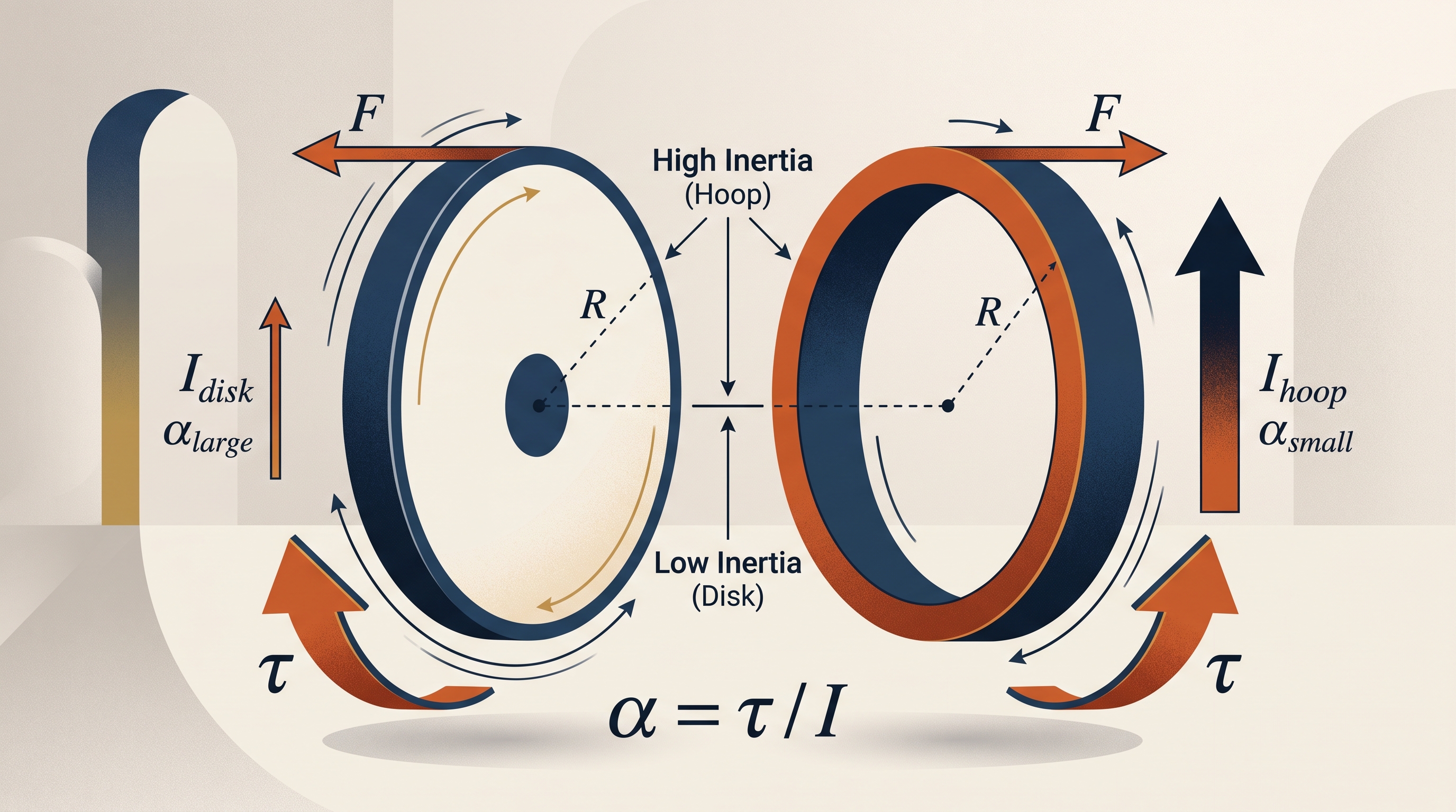
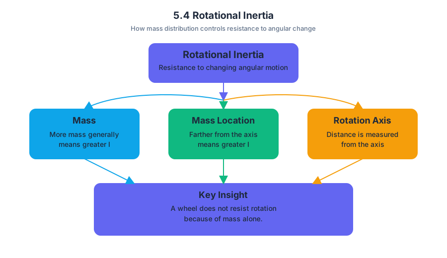
5.5 Rotational Equilibrium and Newton’s First Law in Rotational Form
Key concepts: Rotational equilibrium · Newton’s First Law in rotational form · Translational equilibrium · Net force as a vector sum · Free-body diagrams · Force diagrams · Torque · Forces and torques exerted on an object · Learning objectives and essential knowledge · Science practices: deriving symbolic expressions and applying laws
A rigid object can have zero net torque and still accelerate through space, or have zero net force and still begin rotating. The key is that translational and rotational equilibrium are separate conditions.
5.5 Rotational Equilibrium and Newton’s First Law in Rotational Form
A rigid object can have zero net torque and still accelerate through space, or have zero net force and still begin rotating. The key is that translational and rotational equilibrium are separate conditions.
Learning Objective 5.5.A: Describe the conditions under which a system’s angular velocity remains constant.
Essential Knowledge 5.5.A.1: A system may exhibit rotational equilibrium without being in translational equilibrium, and vice versa.
Two kinds of equilibrium
Translational equilibrium means that the vector sum of all forces on a system is zero:
$$\sum_i \vec{F}_i=\vec{0}$$
Because force is a vector, opposing components cancel separately. Newton’s First Law then says that the system’s velocity remains constant. “Constant” includes both being at rest and moving at constant velocity.
Rotational equilibrium means that the sum of the torques about a chosen axis is zero:
$$\sum_i \tau_i=0$$
The rotational form of Newton’s First Law states that the system’s angular velocity remains constant when the net torque is zero:
$$\sum_i \tau_i=0 \quad \Longrightarrow \quad \omega=\text{constant}$$
Here, constant angular velocity means constant rotational speed and direction about the selected axis.
The two conditions are logically independent:
| Condition | Mathematical test | What remains constant? |
|---|---|---|
| Translational equilibrium | $\sum \vec{F}=\vec{0}$ | Linear velocity $\vec{v}$ |
| Rotational equilibrium | $\sum \tau=0$ | Angular velocity $\omega$ |
| Both | $\sum \vec{F}=\vec{0}$ and $\sum \tau=0$ | Both $\vec{v}$ and $\omega$ |
A system can therefore have $\sum \tau=0$ but $\sum \vec{F}\neq\vec{0}$: it rotates at constant angular velocity while its center of mass accelerates. Conversely, $\sum \vec{F}=0$ but $\sum \tau\neq0$ allows the center of mass to move at constant velocity while the object’s rotation changes.
Reading forces and torques from diagrams
A free-body diagram represents every external force acting on the selected system. A force diagram can additionally emphasize where those forces act and therefore whether they create clockwise or counterclockwise torque. The diagram is not an artistic picture: it is a model of the interaction that must be analyzed.
For each force, ask two questions:
- Does it contribute to the vector sum $\sum \vec{F}$?
- Does its line of action produce a torque about the chosen axis?
A force whose line of action passes through the axis has zero lever arm and therefore produces zero torque about that axis, even though it may contribute substantially to the net force.
Worked example: a balanced beam
A horizontal beam is supported at its center. A person pushes downward with force $120\ \text{N}$ at a point $0.50\ \text{m}$ to the left of the support. Another person pushes downward with force $60\ \text{N}$ at a point $1.00\ \text{m}$ to the right.
Choose counterclockwise torque as positive. The left force produces counterclockwise torque, while the right force produces clockwise torque:
$$\tau_{\text{left}}=(120\ \text{N})(0.50\ \text{m})=60\ \text{N}\cdot\text{m}$$
$$\tau_{\text{right}}=-(60\ \text{N})(1.00\ \text{m})=-60\ \text{N}\cdot\text{m}$$
Therefore,
$$\sum\tau=60-60=0$$
The beam is in rotational equilibrium. If it was initially at rest, it remains at rest rotationally; if it was already rotating, its angular velocity remains constant.
However, the two downward forces add rather than cancel:
$$\sum F_y=-120\ \text{N}-60\ \text{N}=-180\ \text{N}$$
The support must exert an upward force of $180\ \text{N}$ for translational equilibrium. With that support force included, both $\sum \vec{F}=0$ and $\sum\tau=0$.
A common misconception
Misconception: “If the net force is zero, the object cannot rotate.” Zero net force controls the motion of the center of mass, not the rotational motion. Two equal and opposite forces applied along different lines can produce a couple: their forces cancel, but their torques reinforce, so $\sum \tau\neq0$ and the object’s angular velocity changes.
Misconception: “If an object is not rotating, it must be in rotational equilibrium.” An object can be momentarily at rest while experiencing nonzero net torque. In that case, its angular velocity is currently $\omega=0$, but it is about to change. Equilibrium requires $\sum\tau=0$, not merely instantaneous zero angular velocity.
AP skills in this topic
Topic 5.5 is assessed through the Unit 5 progress check and especially develops:
- Science Practice 1—Creating Representations, Skill 1.A: represent the system with a force diagram or free-body diagram, including force locations and torque directions.
- Science Practice 2—Mathematical Routines, Skill 2.B: derive a symbolic expression from a known relationship, such as solving $\sum\tau=0$ for an unknown force or distance.
- Science Practice 3—Scientific Questioning and Argumentation, Skill 3.B: apply an appropriate law, definition, theoretical relationship, or model to make a claim about constant angular velocity.
The AP boundary is deliberate: AP Physics 1 does not expect simultaneous analysis of rotation in multiple planes. Work in one rotational plane, select a clear axis, assign a sign convention, and use the torque sum consistently.
Retrieval check
A wheel experiences a clockwise torque of $8\ \text{N}\cdot\text{m}$ and a counterclockwise torque of $8\ \text{N}\cdot\text{m}$. Is it in rotational equilibrium? What additional information is needed to decide whether it is also in translational equilibrium?
Answer: Yes, because $\sum\tau=0$, so its angular velocity remains constant. The forces themselves must be added as vectors to determine whether $\sum\vec{F}=0$; torque balance alone cannot answer that question.
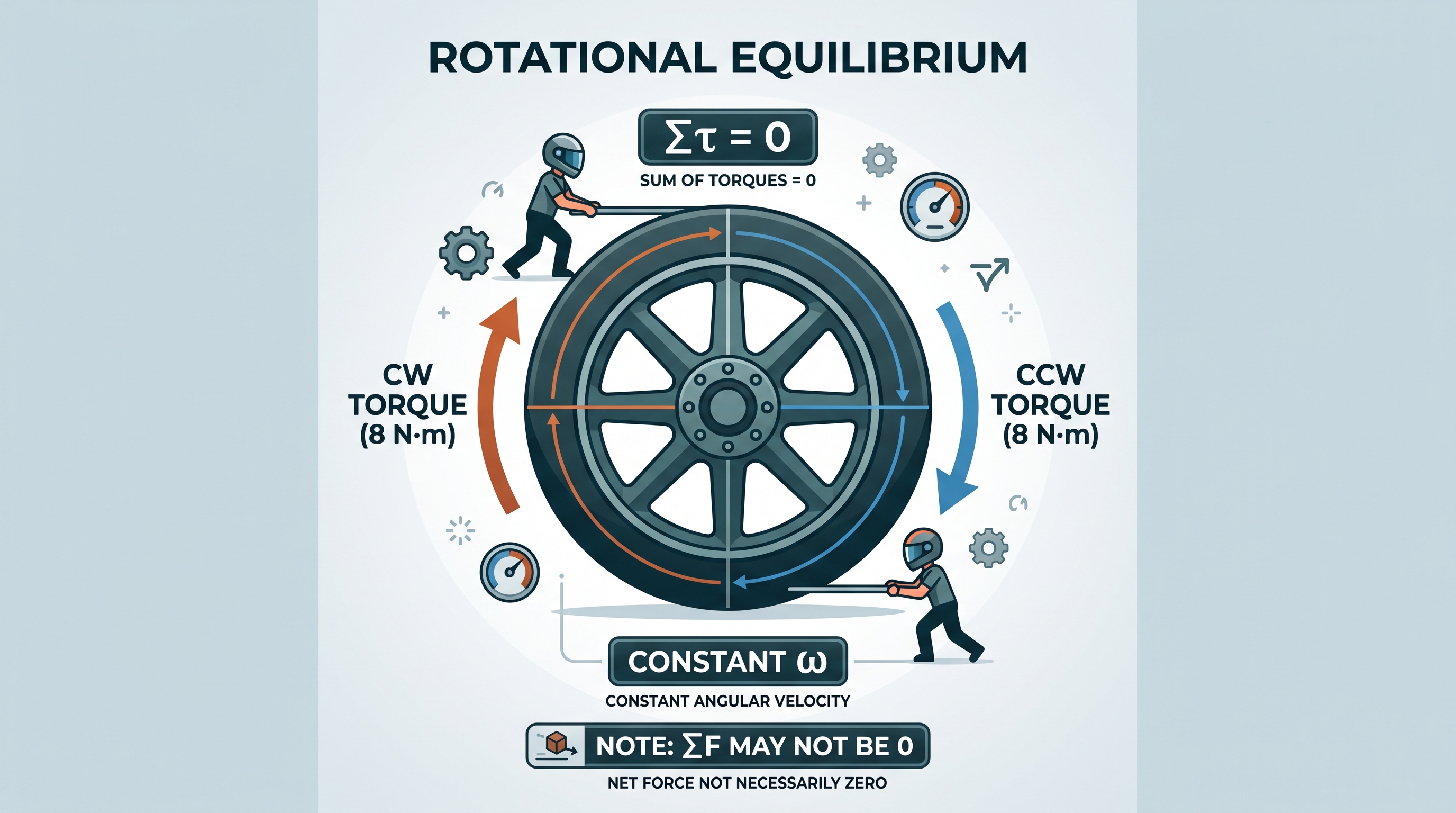
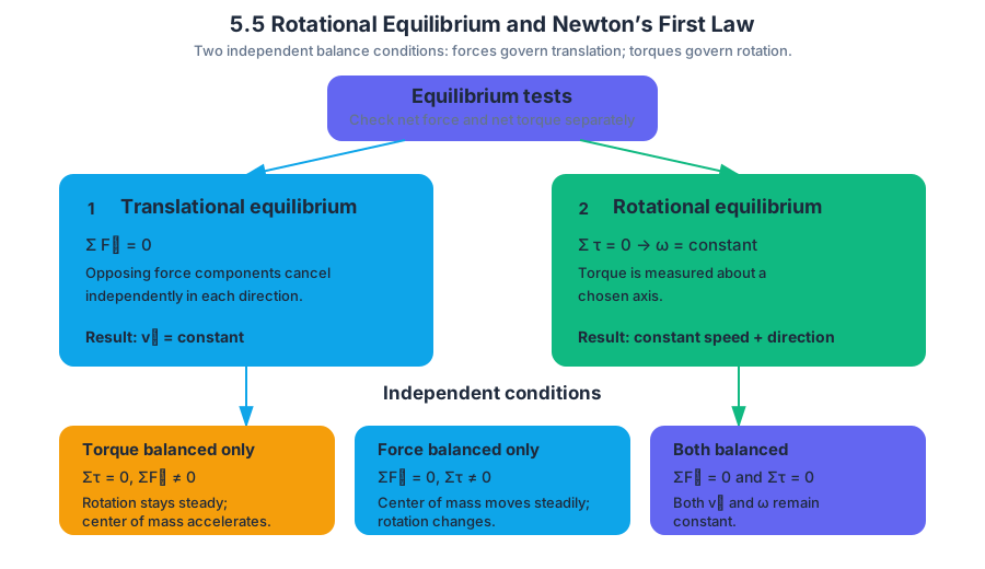
5.6 Newton’s Second Law in Rotational Form
Key concepts: Newton’s second law in rotational form · Net torque and angular acceleration · Rotational inertia · Angular momentum and its rate of change · Angular impulse · Torque produced by friction · Rolling motion on an incline · Single-plane rotation boundary · Qualitative proportional relationships among torque, inertia, and angular acceleration
A rotating object changes its angular velocity when its rotational dynamics produce angular acceleration. For a rigid body rotating about a fixed axis with constant rotational inertia, the cause is the net torque:
5.6 Newton’s Second Law in Rotational Form
A rotating object changes its angular velocity when its rotational dynamics produce angular acceleration. For a rigid body rotating about a fixed axis with constant rotational inertia, the cause is the net torque:
$$\tau_{\text{net}} = I\alpha$$
Here, $\tau_{\text{net}}$ is the sum of torques about the chosen axis, $I$ is rotational inertia—the rotational analogue of mass—and $\alpha$ is angular acceleration.
The rotational cause-and-effect chain
Newton’s second law in rotational form says that torque plays the role of force, rotational inertia plays the role of mass, and angular acceleration plays the role of linear acceleration:
For a fixed-axis rigid body with constant $I$,
$$\alpha = \frac{\tau_{\text{net}}}{I}$$
This creates two important proportional relationships:
- For a given $I$, angular acceleration is directly proportional to $\tau_{\text{net}}$ and points in the same rotational direction.
- For a given $\tau_{\text{net}}$, angular acceleration is inversely proportional to $I$.
Thus, doubling the net torque doubles $\alpha$, while doubling the rotational inertia halves $\alpha$. A nonzero net torque is necessary for a change in angular velocity when the object is rigid, rotates about a fixed axis, and has constant $I$. If $\tau_{\text{net}}=0$, then $\alpha=0$, so $\omega$ remains constant.
Essential Knowledge 5.6.A.2: For a system with constant rotational inertia, $\alpha_{\text{sys}}=\dfrac{\sum \tau}{I_{\text{sys}}}=\dfrac{\tau_{\text{net}}}{I_{\text{sys}}}$.
Torque, angular momentum, and angular impulse
Angular momentum provides the more general statement. For a rigid object rotating about a fixed axis,
$$L=I\omega$$
and the rotational form of Newton’s second law can be written as
$$\tau_{\text{net}}=\frac{dL}{dt}$$
If $I$ is constant, then
$$\tau_{\text{net}}=\frac{d(I\omega)}{dt}=I\frac{d\omega}{dt}=I\alpha$$
Finite-difference forms such as
$$\tau_{\text{net}}=\frac{\Delta L}{\Delta t}=I\frac{\Delta\omega}{\Delta t}=I\alpha$$
are appropriate when the torque and rotational inertia remain constant over the interval, or when the quantities represent suitable average values.
Angular impulse is the accumulated effect of torque over time:
$$\int_{t_1}^{t_2}\tau_{\text{net}},dt=\Delta L$$
Only for constant torque does this reduce to
$$\tau_{\text{net}}\Delta t=\Delta L$$
This explains why a longer-duration torque can produce the same angular-momentum change as a stronger torque acting briefly.
Essential Knowledge 6.3.C.2.ii: The rotational impulse–momentum relationship connects angular impulse to the change in angular momentum.
Important caveat: changing rotational inertia
The statement “zero net torque means constant angular velocity” is not universal. It applies to constant-$I$ rotation. If external torque is zero but the object changes its mass distribution, angular momentum can remain constant while angular velocity changes:
$$L=I\omega=\text{constant}$$
A figure skater who pulls in their arms decreases $I$, so $\omega$ increases even though $\tau_{\text{ext}}=0$. The general law $\tau_{\text{net}}=dL/dt$ handles both constant-$I$ and variable-$I$ motion.
Misconception check — “No net torque means no change in $\omega$.”
That is true only when $I$ is constant. With variable $I$, conservation of angular momentum can require $\omega$ to change.
Worked example: a rolling disk on an incline
A solid disk rolls without slipping down an incline of angle $\theta$. Its rotational inertia about its center is
$$I=\frac{1}{2}MR^2$$
The disk’s center accelerates down the ramp, while friction produces the torque that makes the disk rotate.
Take down the ramp as positive. The forces parallel to the ramp give
$$Mg\sin\theta-F_f=Ma$$
The frictional force produces the net torque about the disk’s center:
$$F_fR=I\alpha$$
Rolling without slipping connects the angular and translational accelerations:
$$\alpha=\frac{a}{R}$$
Substitute both relationships:
$$F_fR=\left(\frac{1}{2}MR^2\right)\left(\frac{a}{R}\right)$$
so
$$F_f=\frac{1}{2}Ma$$
Insert this into the translational equation:
$$Mg\sin\theta-\frac{1}{2}Ma=Ma$$
$$Mg\sin\theta=\frac{3}{2}Ma$$
Therefore,
$$a=\frac{2}{3}g\sin\theta$$
The solution requires both analyses: $\tau_{\text{net}}=I\alpha$ describes the disk’s rotation, while $F_{\text{net}}=Ma$ describes the center of mass. This is the meaning of 5.6.A.3: in complex motion, linear and rotational analyses may need to be performed independently.
Friction and the direction of torque
In the rolling-disk example, gravity’s component $Mg\sin\theta$ pulls the center of mass down the incline, while friction acts in the opposite direction along the ramp. Friction is not automatically “the force that slows motion”; here, its torque is essential to producing the disk’s angular acceleration.
Misconception check — “Friction cannot cause rotation because it acts at the contact point.”
A force produces torque whenever its line of action has a nonzero perpendicular distance from the axis. About the disk’s center, the frictional force has lever arm $R$, so it produces torque.
AP practice lens
This topic develops Science Practice 1: Creating Representations through free-body diagrams and torque diagrams; Science Practice 2: Mathematical Routines through simultaneous equations involving $F_{\text{net}}=Ma$, $\tau_{\text{net}}=I\alpha$, and $\alpha=a/R$; and Science Practice 3: Scientific Questioning and Argumentation through claims about how torque, inertia, and acceleration depend on one another.
Retrieval check: A wheel has constant $I$. If its net torque changes from $3\ \mathrm{N,m}$ to $6\ \mathrm{N,m}$, what happens to $\alpha$? If instead $\tau_{\text{net}}=0$ while $I$ decreases, can $\omega$ change? The answers are: $\alpha$ doubles, and yes—angular momentum conservation can make $\omega$ increase.
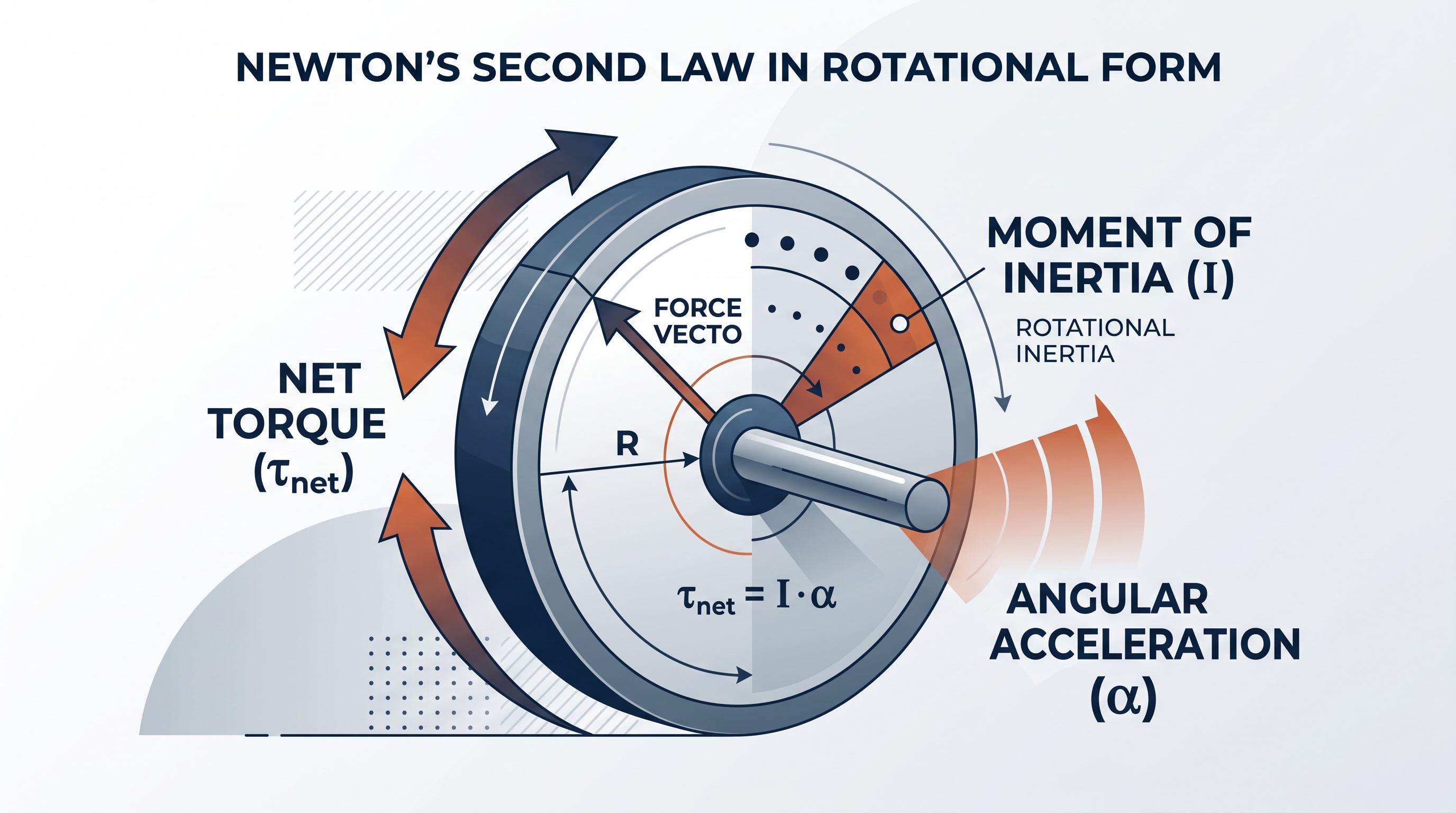
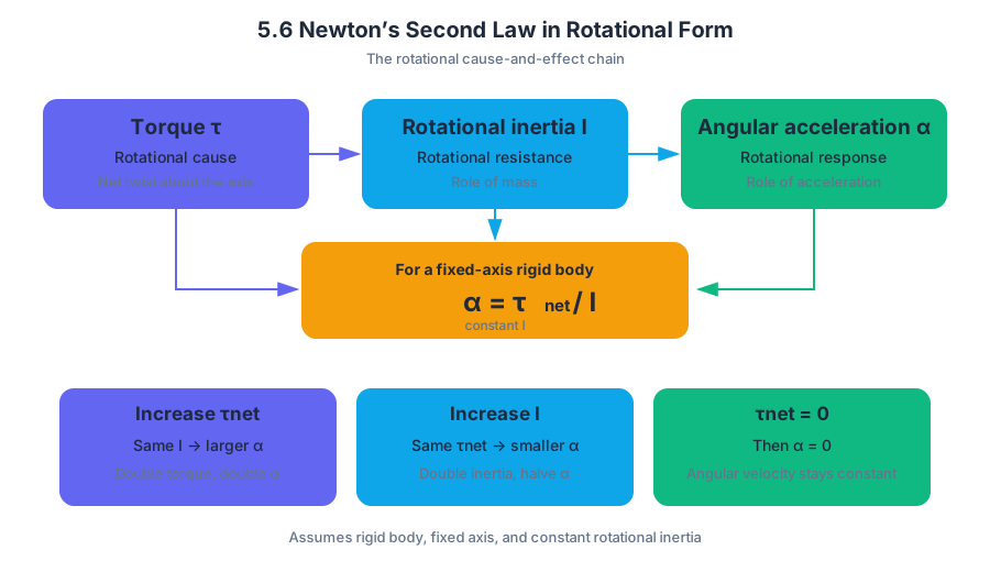
6.1 Rotational Kinetic Energy
Key concepts: Rotational kinetic energy · Translational kinetic energy · Rotational inertia · Energy partition between translational and rotational motion · Conservation of mechanical energy · Rolling motion · Comparison of objects with different rotational inertia · Force and torque analysis of rolling objects · Motion down an incline · Quantitative and qualitative energy representations
A rolling object can arrive at the bottom of an incline with less translational speed than a sliding object because some of its energy is carried by rotation.
6.1 Rotational Kinetic Energy
A rolling object can arrive at the bottom of an incline with less translational speed than a sliding object because some of its energy is carried by rotation. The central question is: when gravity supplies the same energy, how is that energy divided between moving forward and spinning?
Two forms of kinetic energy
Translational kinetic energy is the energy associated with an object’s motion from place to place:
$$K_{\text{trans}}=\frac{1}{2}mv^2$$
Rotational kinetic energy is the energy associated with an object spinning about an axis:
$$K_{\text{rot}}=\frac{1}{2}I\omega^2$$
Here, $m$ is mass, $v$ is the center-of-mass speed, $I$ is rotational inertia—a measure of how difficult it is to change an object’s rotational motion—and $\omega$ is angular speed.
For a frictionless block sliding from rest through a vertical drop $h$, all initial gravitational potential energy becomes translational kinetic energy:
$$mgh=\frac{1}{2}mv^2$$
A rolling disk at the same height has two energy “accounts”:
$$mgh=\frac{1}{2}mv^2+\frac{1}{2}I\omega^2$$
For rolling without slipping, $\omega=v/R$, so if $I=\beta mR^2$,
$$mgh=\frac{1}{2}mv^2(1+\beta)$$
and therefore
$$v=\sqrt{\frac{2gh}{1+\beta}}$$
A larger $\beta$ means more of the available energy is rotational and less is translational.
Worked comparison: block, disk, and ring
Suppose a cart, a solid disk, and a ring have equal mass and radius and start from rest at the same height on identical inclines. Model the cart as primarily translating, the disk as having $I=\frac{1}{2}mR^2$, and the ring as having $I=mR^2$.
| Object | $\beta$ in $I=\beta mR^2$ | Energy partition | Predicted acceleration |
|---|---|---|---|
| Cart | $0$ | Nearly all translational | $g\sin\theta$ |
| Disk | $\frac{1}{2}$ | Translational plus rotational | $\frac{g\sin\theta}{1+\frac{1}{2}}$ |
| Ring | $1$ | Greater rotational share | $\frac{g\sin\theta}{2}$ |
Energy reasoning predicts the cart has the greatest final translational speed, the disk is next, and the ring is slowest. To justify the acceleration and therefore the finishing order, use force and torque reasoning.
For a rolling object on an incline, let $f$ be the static friction force directed up the incline:
$$ma=mg\sin\theta-f$$
The friction force supplies the torque needed for rolling:
$$I\alpha=fR$$
The no-slip condition connects linear and angular acceleration:
$$\alpha=\frac{a}{R}$$
Substituting $I=\beta mR^2$ gives $f=\beta ma$, so
$$ma=mg\sin\theta-\beta ma$$
and
$$a=\frac{g\sin\theta}{1+\beta}$$
Thus the acceleration ranking is
$$a_{\text{cart}}>a_{\text{disk}}>a_{\text{ring}}$$
and, because all begin together and travel the same distance, the predicted order at the bottom is cart first, disk second, ring third. The energy equation explains the final speed ranking; the force-and-torque equations establish the acceleration and travel-time ranking.
Misconception check: “Friction always removes mechanical energy”
Static friction in ideal rolling does not necessarily reduce the system’s total mechanical energy. The contact point is instantaneously at rest relative to the surface, so ideal static friction transfers energy within the object without dissipating it. It is essential for producing the torque that makes the object rotate.
By contrast, kinetic friction during slipping generally converts mechanical energy into thermal energy. The distinction is not “friction versus no friction,” but static rolling contact versus slipping contact.
Ranking three rolling conditions
Consider the same wheel released from rest at the same height and compare its state after descending the same incline:
- Case 1: The track is rough enough for rolling without slipping. Static friction supplies torque, but ideal static friction does no net dissipative work.
- Case 2: The track has some friction, but the wheel slips. Kinetic friction produces rotation while dissipating part of the mechanical energy.
- Case 3: The track has negligible friction. Starting from rest, the wheel receives essentially no frictional torque, so it slides without significant rotation.
Under these specific conditions, the intended rankings are
$$K_{T3}>K_{T2}>K_{T1}$$
$$K_{R1}>K_{R2}>K_{R3}$$
and
$$E_1=E_3>E_2$$
where $K_T$ is translational kinetic energy, $K_R$ is rotational kinetic energy, and $E$ is total mechanical energy. These inequalities depend on the stated initial condition and friction behavior; they are not universal rules for every slipping problem.
AP reasoning in this topic
This topic develops Science Practice 1—Creating Representations, especially energy bar charts and qualitative force-and-torque diagrams. Science Practice 2—Mathematical Routines appears when relating $I$, $\omega$, $m$, $R$, and $v$ algebraically. Science Practice 3—Scientific Questioning and Argumentation is used when defending why one object wins a race or evaluating whether a friction assumption is justified.
The recurring assessment skills are Mathematical Routines, Translation Between Representations, Experimental Design and Analysis, and Qualitative/Quantitative Translation. For example, a student may translate an energy bar chart into an equation, derive a speed ratio, or design a measurement of acceleration and rotational inertia.
Retrieval check
A disk and a ring have equal mass, radius, and starting height and roll without slipping. Which has the smaller translational speed at the bottom, and why?
The ring is slower because its larger rotational inertia gives it a larger rotational share of the fixed gravitational energy. Its acceleration is also smaller because
and the ring has the larger value of $\beta$.
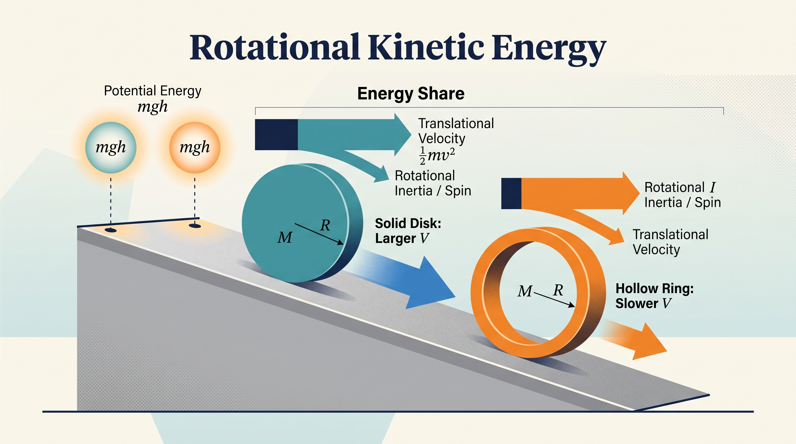
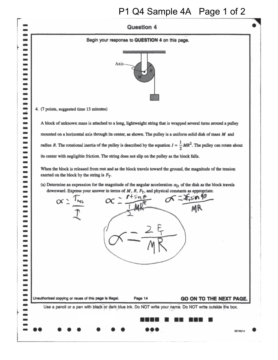
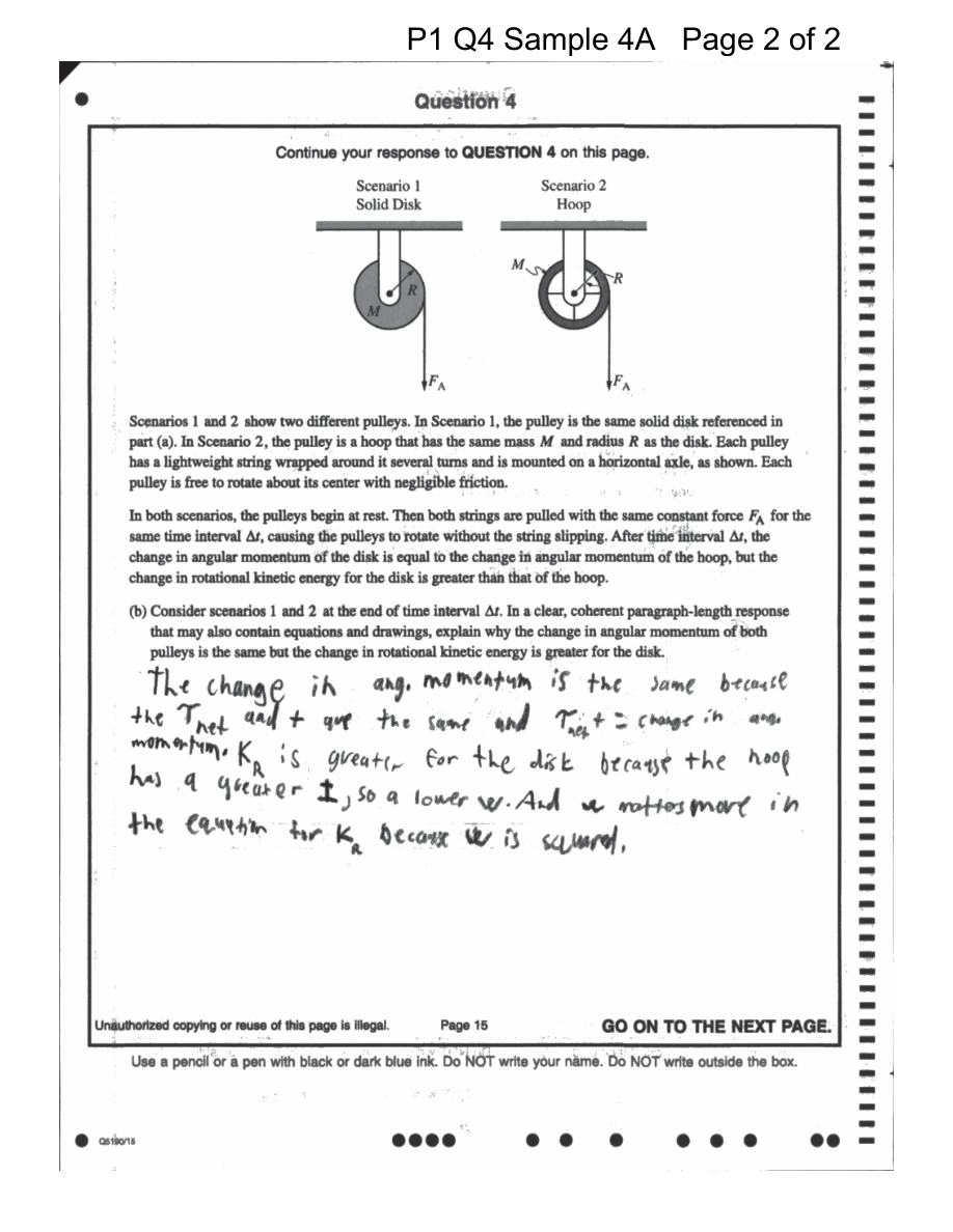
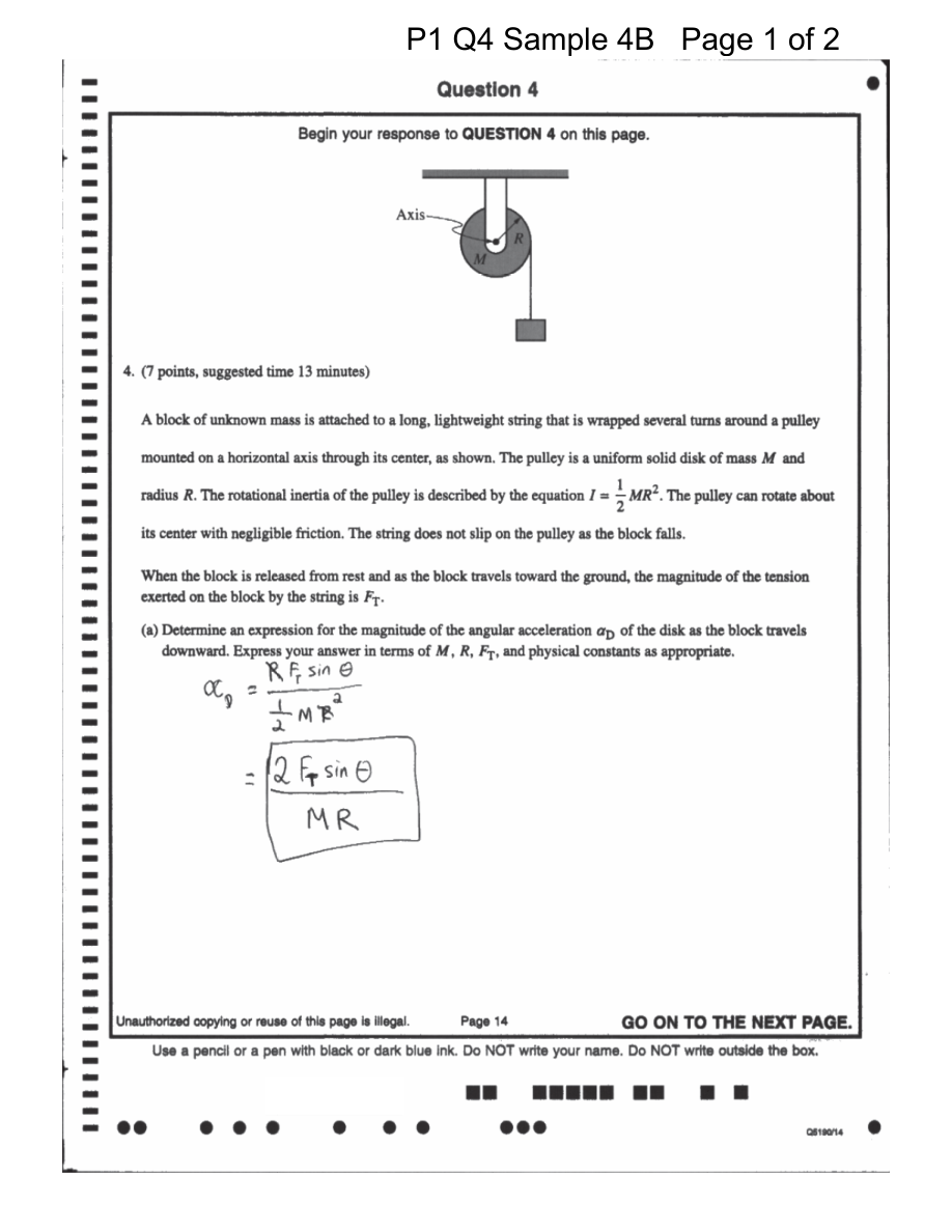
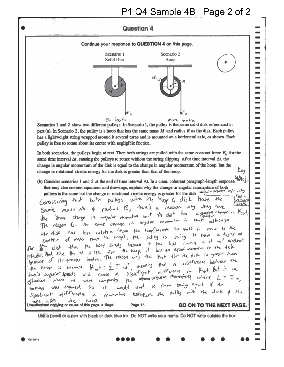
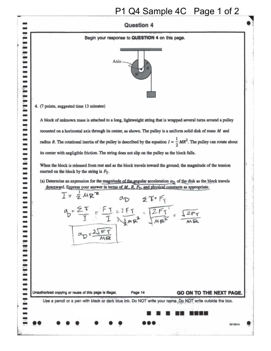
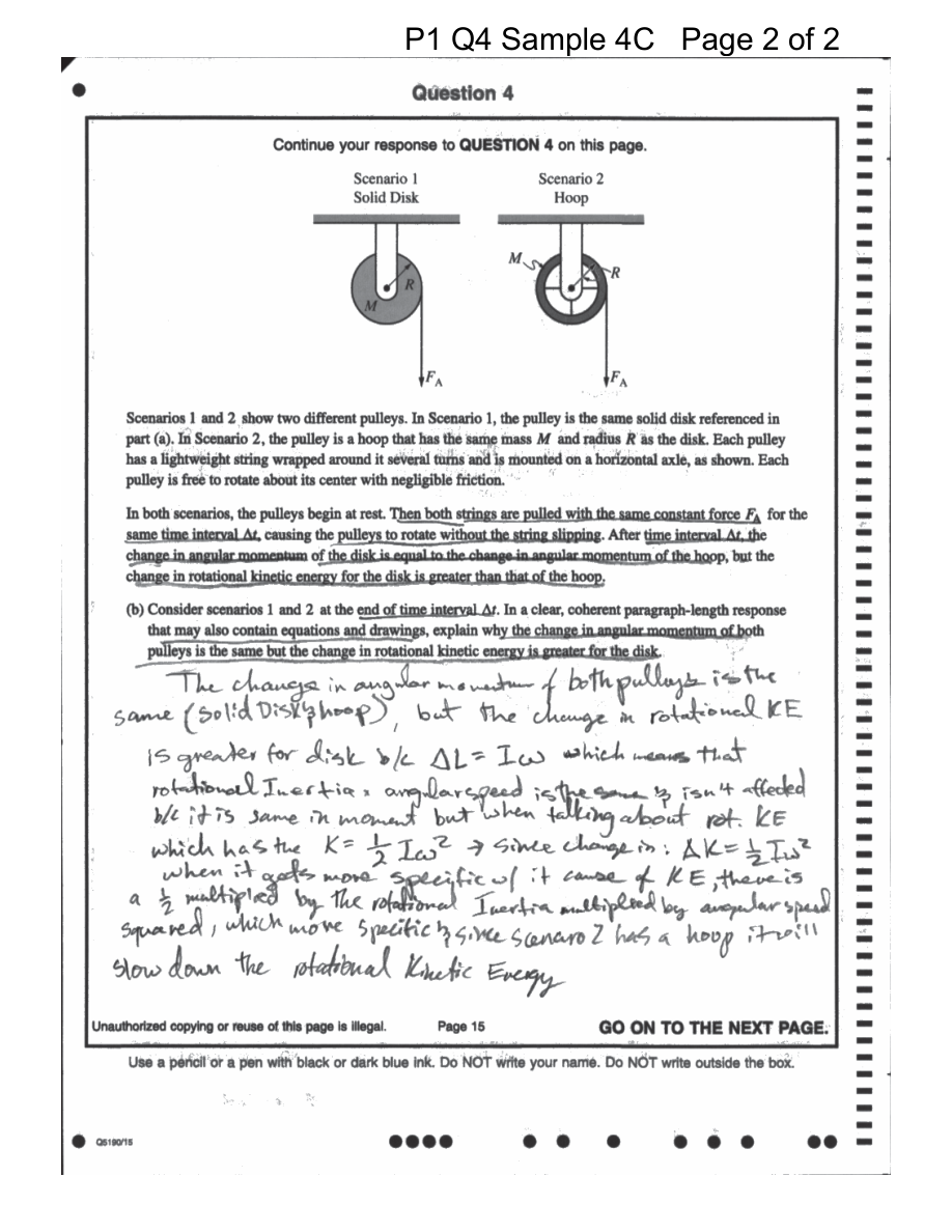
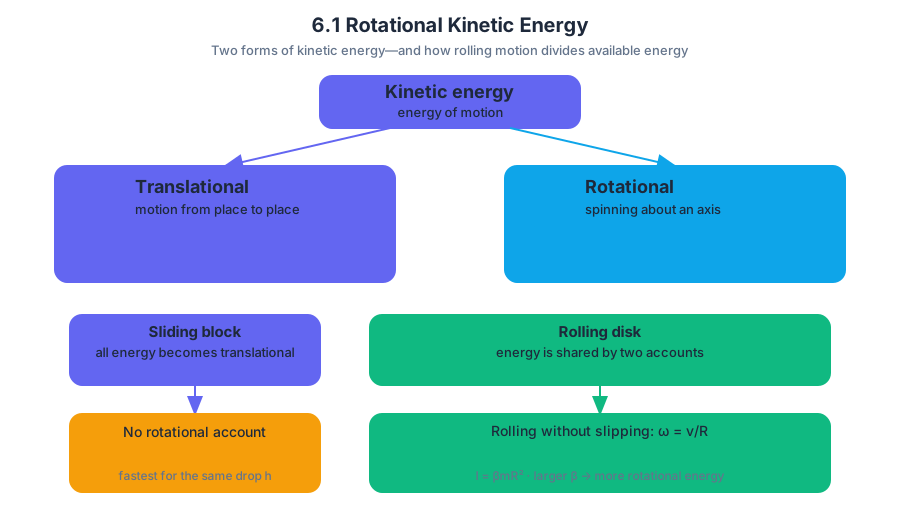
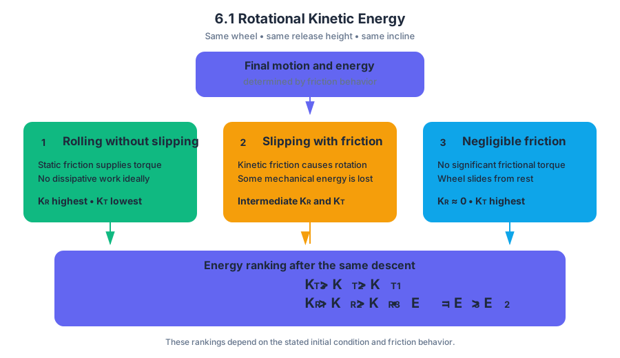
6.2 Torque and Work
A force can make an object move without making it rotate, and it can make an object rotate without doing much translational work. The difference is where the force acts and which part of the displacement is aligned with the force.
6.2 Torque and Work
A force can make an object move without making it rotate, and it can make an object rotate without doing much translational work. The difference is where the force acts and which part of the displacement is aligned with the force.
Imagine opening a heavy door. Pushing near the hinges is difficult because your force has a small lever arm. Pushing at the handle is easier because the same force acts farther from the rotation axis. That rotational effectiveness is called torque.
Torque measures how effectively a force tends to rotate a system about a chosen axis.
For a force perpendicular to a radial line from the axis,
$$\tau = rF$$
where $\tau$ is torque, $r$ is the perpendicular distance from the axis to the force’s line of action, and $F$ is the force magnitude. More generally,
$$\tau = rF\sin\theta$$
where $\theta$ is the angle between the radius vector and the force.
Torque depends on the line of action
The distance that matters is not always the object’s physical radius. It is the lever arm, the shortest perpendicular distance from the rotation axis to the line along which the force acts.
A force directed through the axis has zero lever arm, so it produces no torque:
$$\tau = 0$$
A tangential force produces the greatest torque for a given $r$ and $F$ because $\theta = 90^\circ$ and $\sin 90^\circ = 1$.
Torque is measured in newton-meters, written $\mathrm{N \cdot m}$. Although this has the same base units as a joule, torque and energy are different physical quantities: torque describes rotational influence, while work describes energy transferred by a force.
Torque and rotational work
When a torque turns an object through an angular displacement, it can do rotational work. Work is energy transferred when a force causes displacement in the force’s direction. For constant torque,
$$W = \tau\Delta\theta$$
where $\Delta\theta$ must be measured in radians.
The equation follows from ordinary work. A point at radius $r$ moves through arc length
$$s = r\Delta\theta$$
so a tangential force does work
$$W = Fs = F(r\Delta\theta) = (rF)\Delta\theta = \tau\Delta\theta.$$
If the torque varies during the motion, the constant-torque equation cannot be used with one arbitrary value of $\tau$. The work is represented by the area under a torque-versus-angle graph:
$$W = \int \tau,d\theta.$$
At the algebra-based AP Physics 1 level, the central pattern is to identify whether the torque is constant and then connect rotational work to the change in rotational kinetic energy.
Worked example: turning a flywheel
A motor applies a constant tangential force of $12\ \mathrm{N}$ at the rim of a flywheel of radius $0.25\ \mathrm{m}$. The wheel turns through $8.0\ \mathrm{rad}$. How much work does the motor do?
First find the torque:
$$\tau = rF = (0.25\ \mathrm{m})(12\ \mathrm{N}) = 3.0\ \mathrm{N \cdot m}.$$
Then use the angular work relation:
$$W = \tau\Delta\theta$$
$$W = (3.0\ \mathrm{N \cdot m})(8.0\ \mathrm{rad}) = 24\ \mathrm{J}.$$
The answer is positive because the motor’s torque and the flywheel’s angular displacement point in the same rotational direction. If friction applies an opposing torque, its work is negative and reduces the net energy transferred to the flywheel.
Connecting work to rotational kinetic energy
The work–energy relationship for rotation is
$$W_{\text{net}} = \Delta K_{\text{rot}}.$$
For a rigid object rotating about a fixed axis,
$$K_{\text{rot}} = \frac{1}{2}I\omega^2,$$
so
$$W_{\text{net}} = \frac{1}{2}I\omega_f^2-\frac{1}{2}I\omega_i^2.$$
This connects directly to the rotational kinetic energy model: net torque transfers energy by changing the object’s angular speed.
For constant net torque, combining $W_{\text{net}}=\tau_{\text{net}}\Delta\theta$ with the energy equation gives
$$\tau_{\text{net}}\Delta\theta
\frac{1}{2}I\omega_f^2-\frac{1}{2}I\omega_i^2.$$
This method is often useful when the problem gives angular displacement but not time.
Misconception check: “Torque is rotational force”
Correction: torque is not a separate kind of force. Torque is the rotational effect of an ordinary force about a specified axis. The same force can produce different torques about different axes, and a force can have zero torque about one axis but nonzero torque about another.
A second common error is using degrees in $W=\tau\Delta\theta$. Since arc length satisfies $s=r\theta$, the angle must be in radians. For example, $180^\circ=\pi\ \mathrm{rad}$, not $180$ in the equation.
AP science practices in Topic 6.2
This topic particularly develops Science Practice 1: Creating Representations, including 1.A. Create diagrams, tables, charts, or schematics to represent physical situations. A strong solution sketches the axis, force line of action, lever arm, angular displacement, and positive rotational direction.
It also develops Science Practice 2: Mathematical Routines: 2.A. Derive a symbolic expression from known quantities by selecting and following a logical mathematical pathway, 2.B. Calculate or estimate an unknown quantity with units from known quantities, by selecting and following a logical computational pathway, and 2.C. Compare physical quantities between two or more scenarios or at different times and locations in a single scenario.
For example, doubling $r$ doubles torque, while doubling the angle through which the same torque acts doubles the work. These comparisons require distinguishing the roles of force, lever arm, torque, and angular displacement rather than treating all rotational quantities as interchangeable.
Retrieval check
A wrench is pushed with force $F$ at radius $r$, first perpendicular to the wrench and then at an angle of $30^\circ$ to it. Which case produces greater torque, and by what factor?
The perpendicular case produces
$$\tau_{\perp}=rF,$$
while the angled case produces
$$\tau_{30^\circ}=rF\sin30^\circ=\frac{1}{2}rF.$$
Therefore, the perpendicular push produces twice as much torque.
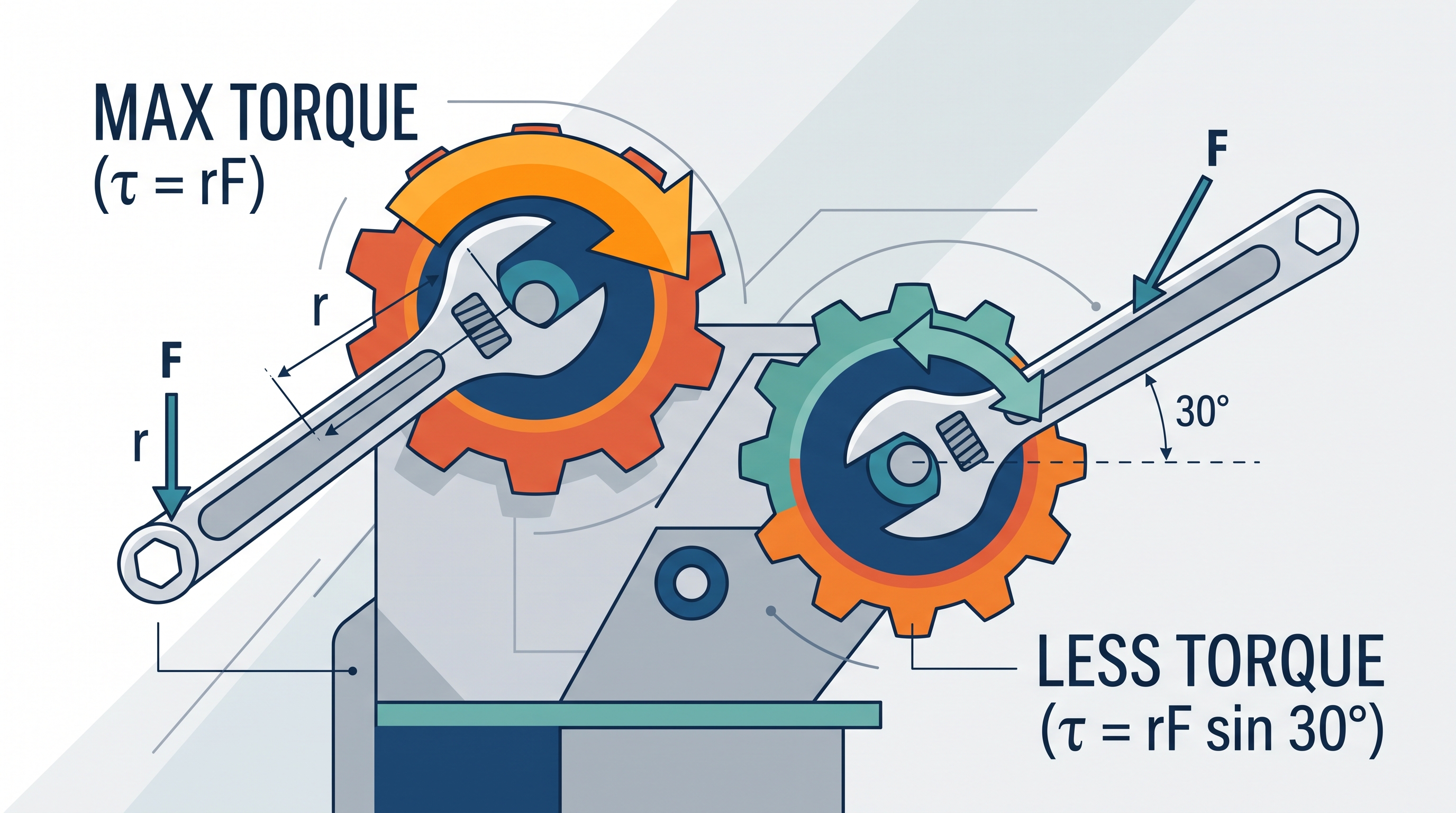
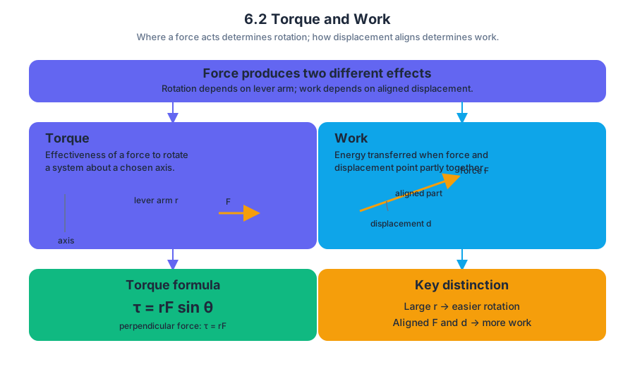
6.3 Angular Momentum and Angular Impulse
Key concepts: Angular momentum · Angular impulse · Rotational impulse–momentum theorem · Torque as the source of angular impulse · Torque-versus-time graphs · Area under a torque–time curve · Change in angular momentum · Direction of torque and angular impulse · Angular impulse delivered to an object or rigid system
A brief twist of a wrench can change a wheel’s rotation, but the important quantity is not torque alone: a torque acting for a time interval delivers angular impulse, changing the object’s angular momentum.
6.3 Angular Momentum and Angular Impulse
A brief twist of a wrench can change a wheel’s rotation, but the important quantity is not torque alone: a torque acting for a time interval delivers angular impulse, changing the object’s angular momentum.
Angular impulse is the accumulated rotational effect of a torque over time. It equals the change in angular momentum:
$$J_{\text{angular}}=\Delta L=L-L_0$$
Here, $L_0$ is the initial angular momentum and $L$ is the final angular momentum. For a rigid object rotating about a fixed axis, angular momentum is often written as $L=I\omega$, where $I$ is rotational inertia and $\omega$ is angular velocity.
6.3.B Angular impulse: torque delivered over time
A torque is the rotational counterpart of a force. When the torque remains constant, its angular impulse is
$$J_{\text{angular}}=\tau\Delta t$$
where $\tau$ is the torque and $\Delta t$ is the interval during which the torque acts. The direction of angular impulse is the same as the direction of the applied torque: a torque that tends to increase counterclockwise rotation produces positive angular impulse if counterclockwise is chosen as positive.
For a torque that varies with time, multiplication is replaced by accumulation:
$$J_{\text{angular}}=\int \tau,dt$$
This integral has a powerful graphical meaning. On a graph of torque $\tau$ versus time $t$, the angular impulse is the signed area under the curve. Area above the time axis represents positive angular impulse; area below it represents negative angular impulse.
The units confirm the connection:
$$[\tau\Delta t]=\left(\mathrm{N,m}\right)\left(\mathrm{s}\right)=\mathrm{N,m,s}$$
Since angular momentum has units $\mathrm{kg,m^2,s^{-1}}$, and $\mathrm{N,m,s}$ reduces to the same dimensions, angular impulse and angular momentum can be related directly.
Reading a torque–time graph
A quantitative graph must have labeled axes, appropriate scales, and units. If a torque–time graph forms a rectangle, triangle, or trapezoid, calculate its area using geometry rather than trying to find a single “average torque” by inspection.
| Torque–time shape | Angular impulse magnitude |
|---|---|
| Rectangle | $J_{\text{angular}}=\tau\Delta t$ |
| Triangle beginning at zero | $J_{\text{angular}}=\frac{1}{2}\tau_{\max}\Delta t$ |
| Trapezoid | $J_{\text{angular}}=\frac{1}{2}(\tau_1+\tau_2)\Delta t$ |
For example, a motor applies a torque that rises linearly from $0\ \mathrm{N,m}$ to $6\ \mathrm{N,m}$ during $4\ \mathrm{s}$. The torque–time graph is a triangle, so
$$J_{\text{angular}}=\frac{1}{2}(6\ \mathrm{N,m})(4\ \mathrm{s})=12\ \mathrm{N,m,s}$$
If the wheel initially has angular momentum $L_0=5\ \mathrm{N,m,s}$ in the positive direction, then
$$L=L_0+J_{\text{angular}}=5+12=17\ \mathrm{N,m,s}$$
The graph’s area, not merely the maximum torque, determines the angular-momentum change.
6.3.C Rotational impulse–momentum theorem
Learning Objective 6.3.C is to relate the change in angular momentum of an object or rigid system to the angular impulse given to that object or rigid system. The rotational impulse–momentum theorem states
$$J_{\text{angular}}=\Delta L$$
and therefore
$$L-L_0=\int \tau_{\text{net}},dt$$
For constant net torque, this becomes
$$\Delta L=\tau_{\text{net}}\Delta t$$
If the rotational inertia is constant, then $L=I\omega$ gives
$$\tau_{\text{net}}=\frac{\Delta L}{\Delta t} =I\frac{\Delta\omega}{\Delta t} =I\alpha$$
The impulse–momentum form is especially useful when the torque acts briefly or changes during the interaction, while $\tau_{\text{net}}=I\alpha$ describes the instantaneous rotational dynamics.
Misconception check: “A larger torque always produces a larger angular impulse”
Not necessarily. Angular impulse depends on both torque and time. A torque of $10\ \mathrm{N,m}$ acting for $1\ \mathrm{s}$ delivers the same angular impulse as a torque of $2\ \mathrm{N,m}$ acting for $5\ \mathrm{s}$:
$$J_{\text{angular}}=(10)(1)=(2)(5)=10\ \mathrm{N,m,s}$$
For changing torque, compare graph areas. A tall, narrow pulse can deliver less angular impulse than a shorter, wider pulse.
AP skills in action
This topic most directly develops Science Practice 1: Creating Representations, especially 1.A Describe representations and models and 1.C Create representations of physical situations, when constructing and interpreting torque–time graphs. It also develops Science Practice 2: Mathematical Routines, especially 2.A Describe relationships mathematically and 2.B Apply mathematical relationships, when using $\Delta L$, $\tau\Delta t$, and geometric area. Science Practice 3: Scientific Questioning and Argumentation appears when a student justifies why two different torque histories produce the same angular-momentum change by comparing their signed areas.
Retrieval check
A torque–time graph has a constant positive torque of $4\ \mathrm{N,m}$ for $3\ \mathrm{s}$, followed by a constant negative torque of $2\ \mathrm{N,m}$ for $2\ \mathrm{s}$. What is the net angular impulse?
The signed area is
$$J_{\text{angular}}=(4)(3)-(2)(2)=8\ \mathrm{N,m,s}$$
So the object’s angular momentum increases by $8\ \mathrm{N,m,s}$ in the positive direction.
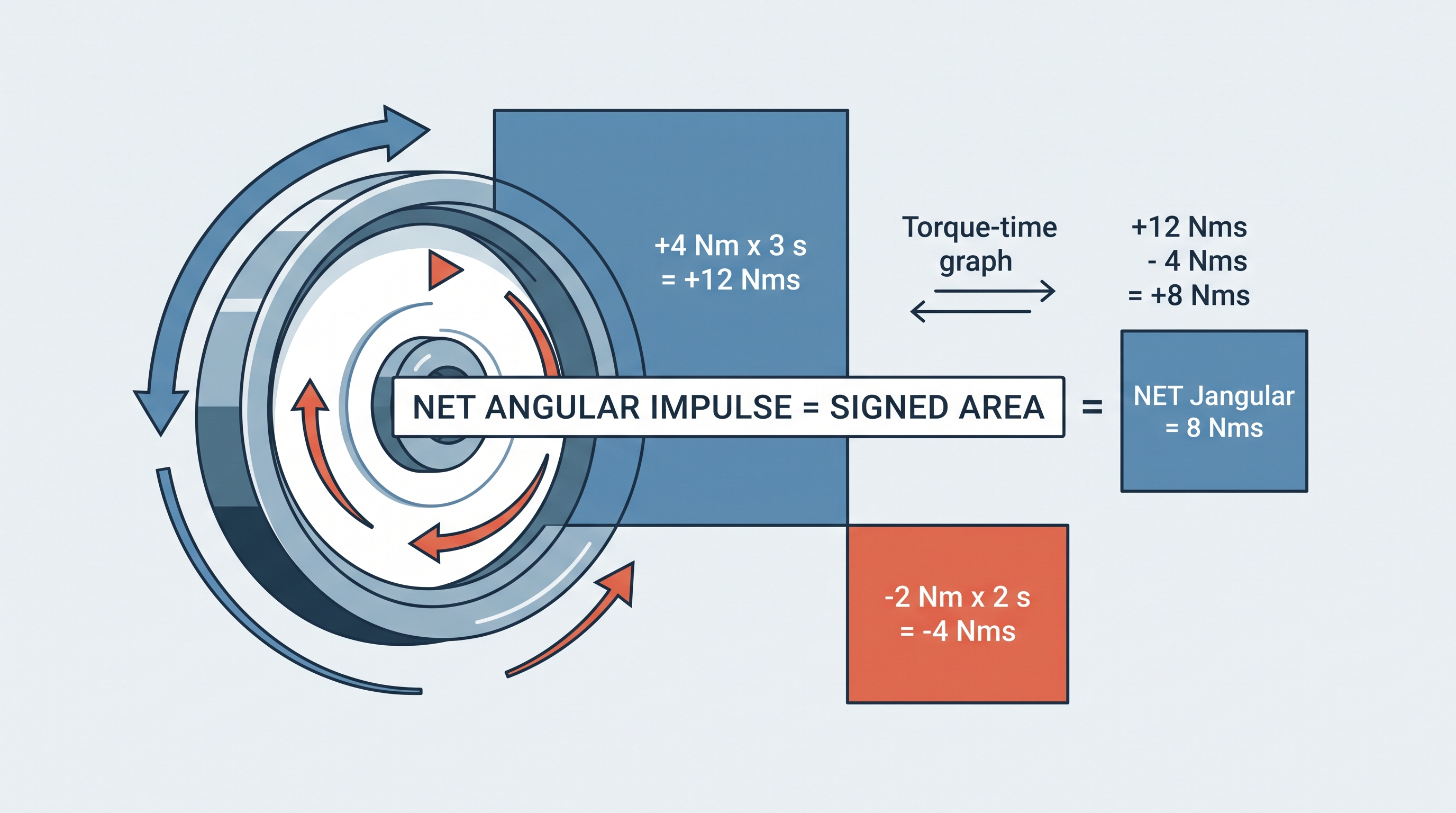
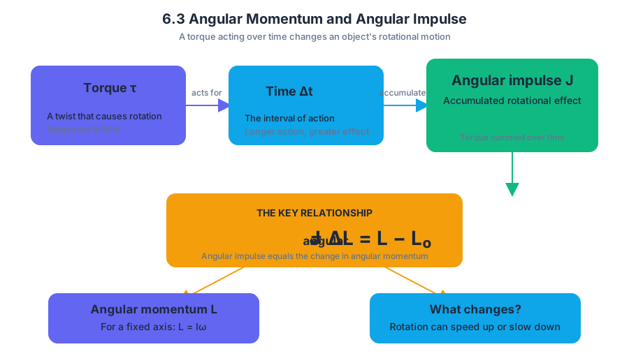
6.4 Conservation of Angular Momentum
Key concepts: Angular momentum conservation · Net external torque and its role in conservation · System boundaries and the environment · Transfer of angular momentum · Angular momentum of orbiting objects · Relationship between orbital radius and tangential speed · Torque versus force in rotational dynamics · Block-spring systems involving rotation and energy
Angular momentum stays constant only when the chosen system experiences zero net external torque over the interval being analyzed.
6.4 Conservation of Angular Momentum
Angular momentum stays constant only when the chosen system experiences zero net external torque over the interval being analyzed.
Learning Objective 6.4.B: Make predictions about the angular momentum of a selected object or rigid system by identifying the system boundary and evaluating the external torque acting on it.
The system boundary decides what “conserved” means
A system is the object or collection of objects you choose to analyze. Everything not included is the environment. A torque caused by an object inside the system is internal; a torque caused by something outside it is external.
| System choice | Torque classification | What can be conserved? |
|---|---|---|
| A spinning student alone | The floor or another person may exert external torque | The student’s angular momentum can change |
| Student plus rotating stool | Friction between them is internal | Their combined angular momentum can remain constant if outside torque is negligible |
| Two objects interacting only through gravity | Gravitational torques are internal | The pair’s total angular momentum is conserved |
Essential Knowledge 6.4.B.1 expresses the universal conservation idea: angular momentum is not destroyed. It can move between parts of a larger system. Whether the angular momentum of your selected system remains constant depends on whether the environment transfers angular momentum into or out of it.
Torque determines the change
Essential Knowledge 6.4.B.2 gives the conservation condition. For a selected object or rigid system,
$$ \frac{dL}{dt}=\tau_{\text{net, external}}. $$
If the net external torque is zero at every instant, then the angular momentum remains constant. More generally, the change during a finite time interval depends on the net external angular impulse:
$$ \Delta L=\int_{t_i}^{t_f}\tau_{\text{net, external}},dt. $$
Thus, a nonzero external torque means that angular momentum is changing instantaneously at that moment. It does not guarantee a nonzero final change over an entire interval: positive and negative torques can cancel, giving zero net angular impulse and therefore $\Delta L=0$.
Essential Knowledge 6.4.B.3: If the net external torque on a selected object or rigid system is nonzero, angular momentum is transferred between the system and the environment.
Misconception check — “Any torque means angular momentum is permanently lost.” Torque is not a loss mechanism. It is the mechanism by which angular momentum crosses the system boundary. If the environment exerts a positive torque, the system gains angular momentum; if it exerts a negative torque, the system gives angular momentum back.
Orbiting objects: radius and tangential speed
For an object moving perpendicular to its radius from the rotation axis, angular momentum can be written as
$$ L=rp, $$
where $r$ is the orbital radius and $p$ is linear momentum. Since $p=mv$,
$$ L=rmv. $$
For a fixed mass in an isolated system, conservation gives
$$ r_i m v_i=r_f m v_f, $$
so
$$ r_i v_i=r_f v_f. $$
If the orbital radius decreases, the tangential speed must increase. If the radius doubles, the tangential speed becomes half as large, provided the angular momentum remains constant.
A useful application is two objects interacting only through gravitational forces. If the two-object pair is the system, gravity is internal, so the pair’s total angular momentum can be conserved. If only one object is selected, the gravitational force from the other object is external, and that object’s angular momentum may change.
A torque calculation must use the actual applied force
For a rotating disk, the torque from a tangential force is determined by the force and its lever arm:
$$ \tau=rF_T, $$
when the force is perpendicular to the radius. The lever arm is the perpendicular distance from the axis to the force’s line of action.
If a string pulls the disk with force $F_T$, the disk’s torque is based on $F_T$, not directly on the gravitational force $m g$ acting on a hanging block. The block’s weight may help determine $F_T$ through a separate force analysis, but it is not automatically the torque-producing force on the disk.
Likewise, a spring’s energy can relate stretch distance to a block’s speed through conservation of energy, but that does not replace the correct angular-momentum or torque equation for the rotating disk.
AP reasoning in action
This topic develops Science Practice 1—Creating Representations when you draw the system boundary, identify the environment, and represent internal versus external torques. It develops Science Practice 2—Mathematical Routines when you apply $L=rp$, $\frac{dL}{dt}=\tau_{\text{net, external}}$, or $\Delta L=\int \tau,dt$. It develops Science Practice 3—Scientific Questioning and Argumentation when you use evidence from a diagram, graph, or experiment to justify a claim about conservation. The associated reasoning skill is Qualitative/Quantitative Translation: turn “smaller radius means faster tangential motion” into $r_i v_i=r_f v_f$.
Retrieval check: A satellite moves to a smaller orbital radius while its system’s angular momentum remains constant. What happens to its tangential speed, and what condition justifies your answer?
Answer: Its tangential speed increases because $r v$ is constant when the mass is fixed and the net external torque on the chosen system is zero.
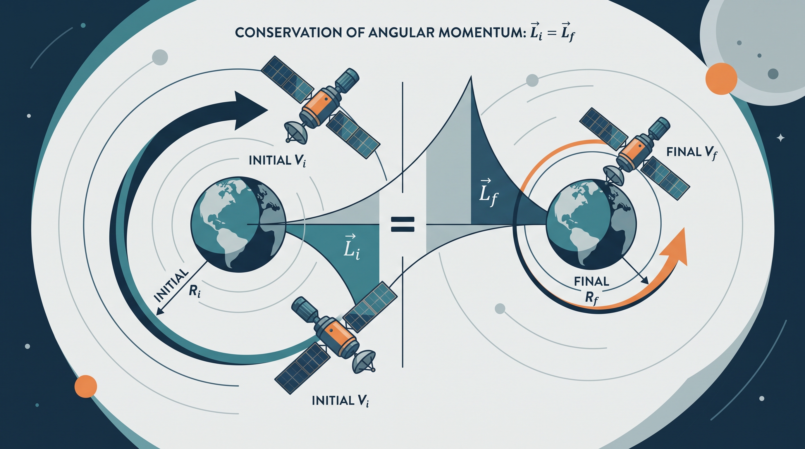

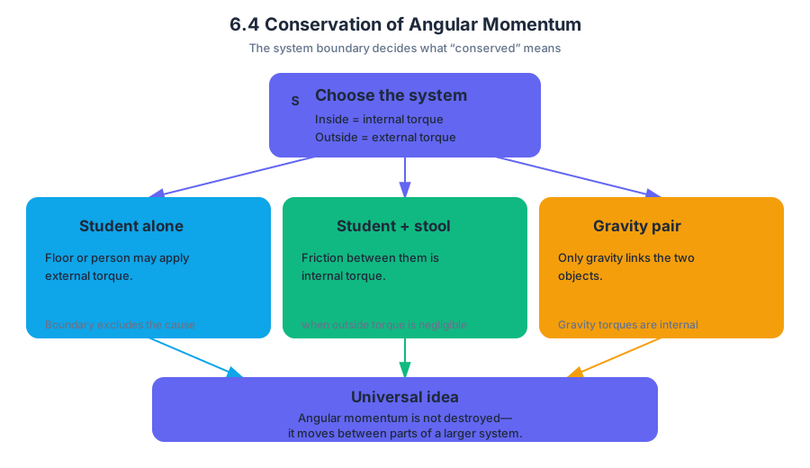
6.5 Rolling
A rolling object moves forward while rotating, so its motion combines translation of its center of mass with rotation about its center. A bicycle tire, a bowling ball, and a wheel on a ramp all obey the same central condition when they roll without slipping:
6.5 Rolling
A rolling object moves forward while rotating, so its motion combines translation of its center of mass with rotation about its center. A bicycle tire, a bowling ball, and a wheel on a ramp all obey the same central condition when they roll without slipping:
$$v_{\mathrm{cm}} = R\omega$$
Here, $v_{\mathrm{cm}}$ is the speed of the center of mass, $R$ is the radius, and $\omega$ is the angular speed.
The condition means that the point of contact with the surface is instantaneously at rest relative to the surface. The center moves forward at speed $v_{\mathrm{cm}}$, while rotation gives the contact point a backward tangential speed $R\omega$; these cancel exactly.
Rolling without slipping
Rolling without slipping is a kinematic constraint, not a new kind of energy. It connects linear and angular variables:
$$s = R\theta,\qquad v_{\mathrm{cm}} = R\omega,\qquad a_{\mathrm{cm}} = R\alpha$$
The angle $\theta$ must be measured in radians. These equations apply when the object maintains contact and does not slide across the surface.
A rough surface is essential: static friction must be large enough to prevent slipping. In the ideal model, however, static friction does no work because the point where the friction force acts has zero instantaneous velocity relative to the surface. Static friction can still change the object’s translational and rotational kinetic energies separately; it simply transfers energy between those forms rather than removing mechanical energy.
Key idea: Static friction supplies the torque needed for rolling, while ideal static friction does no net work on the rolling object.
Energy of a rolling object
A rolling object has two kinetic-energy terms:
$$K = K_{\mathrm{trans}} + K_{\mathrm{rot}}$$
$$K = \frac{1}{2}Mv_{\mathrm{cm}}^2+\frac{1}{2}I\omega^2$$
Using $\omega = v_{\mathrm{cm}}/R$ gives
$$K=\frac{1}{2}Mv_{\mathrm{cm}}^2+\frac{1}{2}\frac{I}{R^2}v_{\mathrm{cm}}^2$$
The rotational inertia $I$ determines how much of the object’s energy is tied up in rotation.
For an object rolling down a ramp that is rough enough to enforce rolling without slipping but produces no energy loss, gravitational potential energy becomes both translational and rotational kinetic energy:
$$Mgh=\frac{1}{2}Mv_{\mathrm{cm}}^2+\frac{1}{2}I\omega^2$$
If the object starts from rest and drops through height $h$, then
$$v_{\mathrm{cm}}=\sqrt{\frac{2Mgh}{M+I/R^2}}$$
A smaller value of $I/(MR^2)$ produces a greater final speed.
Worked example: comparing rolling objects
A solid disk and a thin hoop have the same mass, radius, and starting height. Both roll without slipping down the same ramp. Which reaches the bottom with greater speed?
For a solid disk,
$$I_{\mathrm{disk}}=\frac{1}{2}MR^2$$
For a thin hoop,
$$I_{\mathrm{hoop}}=MR^2$$
The disk therefore has
$$v_{\mathrm{disk}}=\sqrt{\frac{2Mgh}{M+\frac{1}{2}M}} =\sqrt{\frac{4gh}{3}}$$
The hoop has
$$v_{\mathrm{hoop}}=\sqrt{\frac{2Mgh}{M+M}} =\sqrt{gh}$$
Since $\sqrt{4gh/3}>\sqrt{gh}$, the solid disk reaches the bottom faster. The disk’s mass is distributed closer to its axis, so it has less rotational inertia and requires less energy for rotation at a given translational speed.
This comparison does not mean the disk experiences a greater gravitational force. Both objects have the same weight. Their different speeds result from how their mass distribution divides the available energy between translation and rotation.
Acceleration down a ramp
For an object rolling down an incline of angle $\phi$, the acceleration of its center of mass is
$$a_{\mathrm{cm}}=\frac{g\sin\phi}{1+\frac{I}{MR^2}}$$
The denominator captures rotational resistance. For a solid sphere, $I/(MR^2)=2/5$; for a solid disk, it is $1/2$; for a hoop, it is $1$. Thus, on the same ramp,
$$a_{\mathrm{sphere}}>a_{\mathrm{disk}}>a_{\mathrm{hoop}}$$
The rolling object with more mass concentrated farther from its axis accelerates more slowly.
Misconception check — “Friction always opposes motion and removes energy.” Friction opposes slipping, not necessarily the center-of-mass motion. In ideal rolling, static friction provides the torque that establishes the required angular acceleration, but it does not dissipate mechanical energy. If the object actually slips, kinetic friction acts, mechanical energy is converted into thermal energy, and the relation $v_{\mathrm{cm}}=R\omega$ no longer holds.
Retrieval check: A hoop and a solid sphere roll from rest down identical ramps without slipping. Without calculating, identify which has the greater final speed and explain why. The solid sphere is faster because its smaller ratio $I/(MR^2)$ leaves more of the gravitational energy available for translational motion.
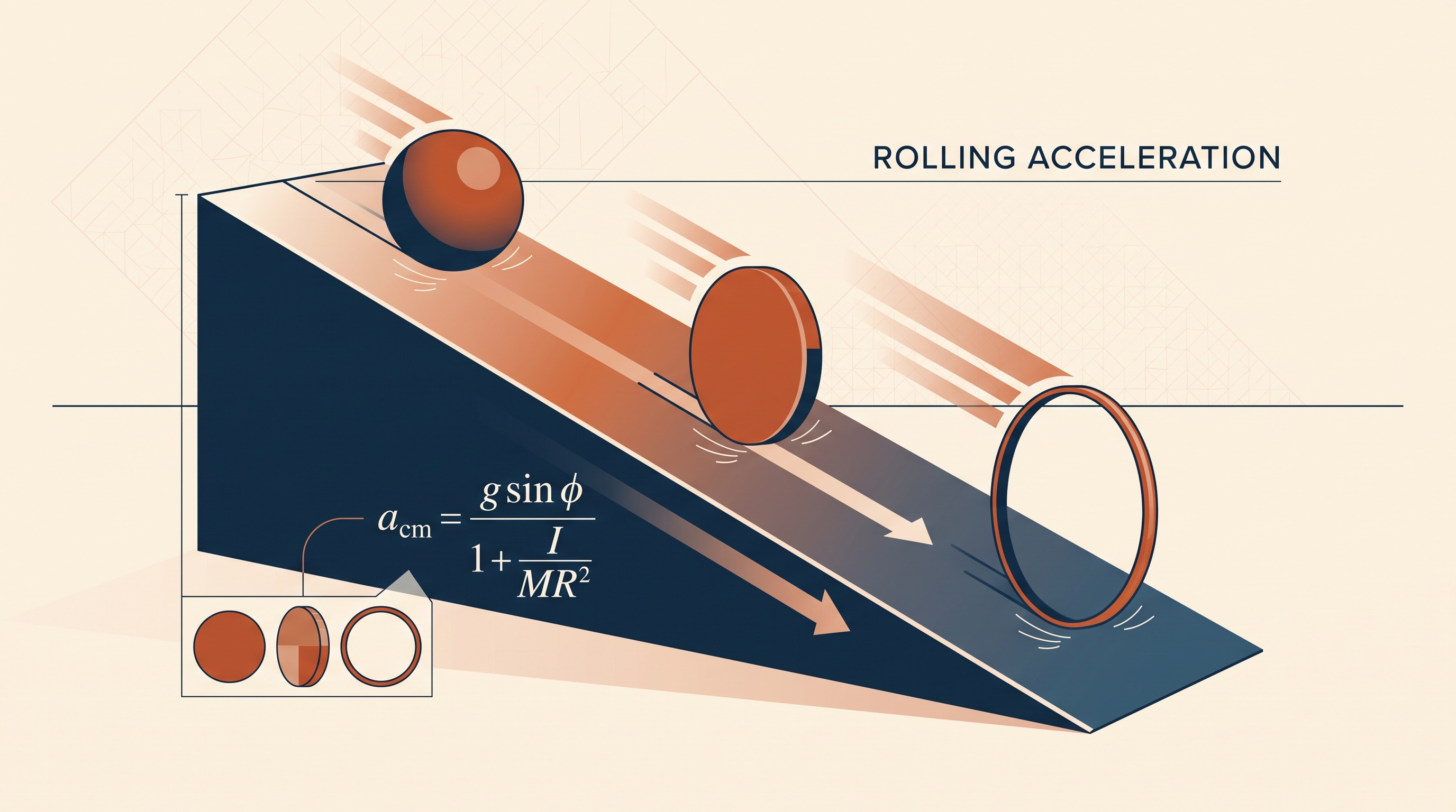
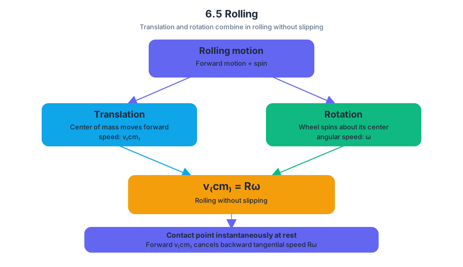
6.6 Motion of Orbiting Satellites
Key concepts: Rolling while slipping · Relative motion between the contact point and the surface · Kinetic friction · Energy dissipation due to kinetic friction · Mechanical-energy loss · Forces and torques in qualitative modeling · Motion of orbiting satellites · Gravitational force
An orbiting satellite is continuously falling toward a massive central object, but its sideways motion carries it forward so that it keeps missing the object.
6.6 Motion of Orbiting Satellites
An orbiting satellite is continuously falling toward a massive central object, but its sideways motion carries it forward so that it keeps missing the object. A different kind of motion appears when a rotating object slips against a surface: kinetic friction then acts at a contact point that moves relative to the surface, removing mechanical energy.
Orbiting satellites: gravity supplies the centripetal force
For a system containing a massive central object and a satellite whose mass is negligible compared with it, the central object’s motion can be treated as negligible. The satellite’s acceleration points toward the central object, so the inward gravitational force provides the centripetal force required for circular motion.
Essential Knowledge 6.6.A.1: In a system consisting only of a massive central object and an orbiting satellite with mass that is negligible in comparison to the central object’s mass, the motion of the central object itself is negligible.
For a circular orbit of radius $r$, the gravitational force and centripetal-force requirement describe the same inward interaction:
$$ F_g = \frac{G M m}{r^2} $$
$$ F_{\text{net,inward}} = \frac{m v^2}{r} $$
Therefore,
$$ \frac{G M m}{r^2}=\frac{m v^2}{r}. $$
The satellite’s mass cancels:
$$ v=\sqrt{\frac{G M}{r}}. $$
This result gives an important qualitative conclusion: a satellite in a larger circular orbit moves more slowly, not faster. The inward force is smaller at larger $r$, and the required orbital speed is also smaller.
The force model is compact:
- The satellite experiences a gravitational force directed toward the central object.
- The satellite’s velocity is tangent to the orbit.
- The inward acceleration changes the direction of velocity continuously.
- In an ideal circular orbit, gravity does no work because the force is perpendicular to the instantaneous displacement.
- The satellite therefore maintains constant speed while its velocity changes direction.
Worked example: comparing two circular orbits
A satellite moves from a circular orbit of radius $r$ to one of radius $4r$ around the same central object. Using $v=\sqrt{GM/r}$,
$$ \frac{v_2}{v_1}
\sqrt{\frac{GM/(4r)}{GM/r}}
\frac{1}{2}. $$
The satellite in the larger orbit has half the speed. Its gravitational force is also one-sixteenth as large because $F_g\propto r^{-2}$, while its required centripetal acceleration is one-fourth as large because $a_c=v^2/r$.
Misconception check — “A satellite needs a forward force to keep orbiting.”
It does not need a separate forward force in the ideal model. Its tangential velocity carries it forward; gravity continually bends that velocity inward. If gravity disappeared, the satellite would move in a straight line tangent to the orbit.
Rolling while slipping: where kinetic friction does work
A rotating system is rolling while slipping when it both rotates and translates, but the point of contact does not remain instantaneously at rest relative to the surface. The pure-rolling condition established earlier is therefore violated: the contact point and the surface have relative motion.
Essential Knowledge 6.5.C.2: When a rotating system is slipping relative to another surface, the point of application of the force of kinetic friction exerted on the system moves with respect to the surface, so the force of kinetic friction will dissipate energy from the system.
Because the contact point moves relative to the surface, kinetic friction does work. Friction usually points opposite the relative sliding, so the work done by friction on the mechanical system is negative:
$$ W_f<0. $$
That negative work transfers energy into thermal energy and decreases the system’s mechanical energy:
$$ \Delta E_{\text{mech}}=W_{\text{nonconservative}}<0. $$
The force can also produce a torque about the object’s center of mass. Thus slipping friction may change both the object’s translational speed and its angular speed.
Qualitative force-and-torque model
Imagine a bowling ball thrown forward with almost no spin. The bottom of the ball initially slides forward relative to the floor. Kinetic friction acts backward on the ball, reducing its linear speed, while the frictional torque increases its angular speed in the direction needed for rolling. The slipping decreases until the translational and rotational motions satisfy the pure-rolling condition.
The reverse can occur if a ball spins too rapidly for its forward speed. Friction then acts in the opposite horizontal direction, changing the linear and angular motion in the opposite senses. The exact time dependence is beyond the required qualitative model; the essential prediction is that kinetic friction opposes relative motion, produces a torque, and dissipates mechanical energy.
Boundary statement: Rolling friction—the resistance associated with an object that is already rolling without slipping—is beyond the scope of AP Physics 1. The relevant energy loss here comes from kinetic friction during slipping.
Skill connection and retrieval check
The satellite model is assessed through Science Practice 1, Skill 1.C: Create qualitative sketches of graphs that represent features of a model or physical situation. A useful sketch should show a satellite’s tangential velocity and inward gravitational force separately, or show how orbital speed varies qualitatively with orbital radius. For slipping, a force diagram plus a torque arrow communicates why linear and angular speeds change together but not identically.
Retrieval check: A satellite’s orbital radius increases while it remains in a circular orbit. Does its speed increase or decrease, and why? A disk slides to the right while rotating too slowly for rolling. Which way does kinetic friction act, and what happens qualitatively to its linear speed, angular speed, and mechanical energy?
Answers: The satellite’s speed decreases because $v\propto r^{-1/2}$. For the disk, friction acts opposite the relative sliding at the contact point; it reduces the sliding and changes the disk’s translation and rotation through force and torque. Its mechanical energy decreases because kinetic friction does negative work.
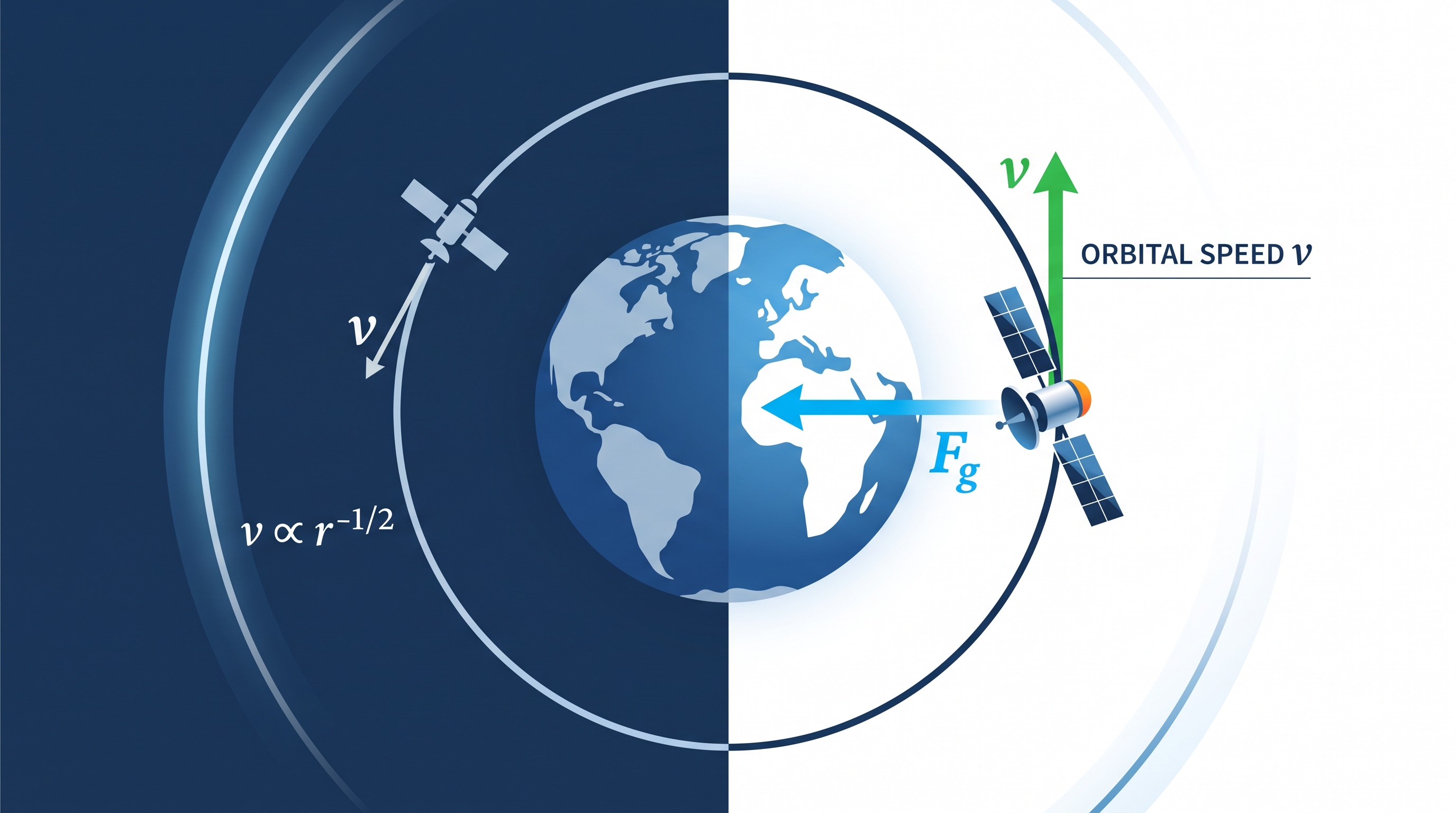
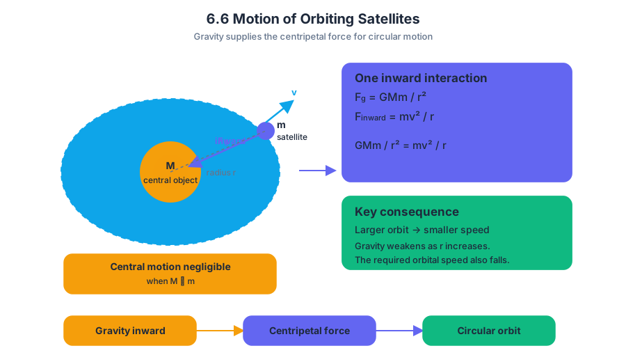
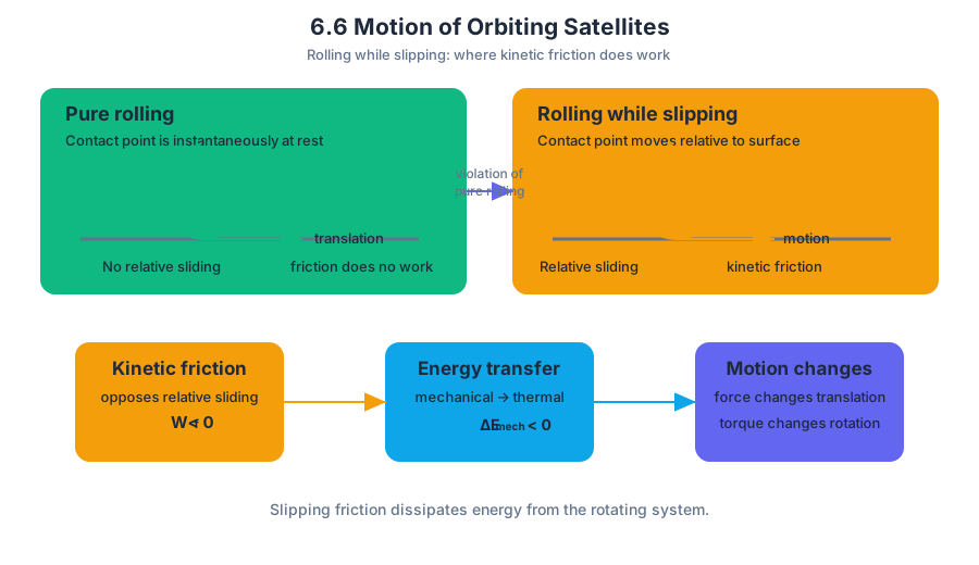
Unit 7: Oscillations — Exam-Style Practice
Exam-style free-response practice for AP Physics 1 Unit 7: simple harmonic motion, its frequency and period, representing and analyzing SHM, and the energy of simple harmonic oscillators.
Unit 7: Oscillations — Exam-Style Practice
This page collects exam-style free-response questions for AP Physics 1 Unit 7:
- 7.1 Defining Simple Harmonic Motion
- 7.2 Frequency and Period of SHM
- 7.3 Representing and Analyzing SHM
- 7.4 Energy of Simple Harmonic Oscillators
Write your answer to each part, then compare it with the model answer.
8.1 Internal Structure and Density
Key concepts: Internal structure and density · Fluids as the subject of Unit 8
A fluid can flow because its particles are not locked into a fixed shape, but the particles still occupy space and contribute mass. Density measures how much mass is packed into a given volume:
8.1 Internal Structure and Density
A fluid can flow because its particles are not locked into a fixed shape, but the particles still occupy space and contribute mass. Density measures how much mass is packed into a given volume:
$$\rho=\frac{m}{V}$$
where $\rho$ is density, $m$ is mass, and $V$ is volume. Density is therefore an intensive property: doubling the amount of a uniform material doubles both its mass and volume, leaving $\rho$ unchanged.
Internal structure: what makes a fluid a fluid?
Imagine a crowd of people in a room. In a solid, each person is constrained to a particular position relative to nearby people; the group keeps its shape. In a fluid, the particles remain close enough to interact but can rearrange and slide past one another. A liquid keeps nearly the same volume while changing shape to fit its container; a gas spreads out to occupy the available container volume.
The microscopic picture explains why density depends on both the material and its physical state. A tightly packed sample has more mass in each cubic meter than a loosely packed sample. Heating, compressing, or changing a substance’s phase can alter the spacing of its particles and therefore change its density.
Density is mass per unit volume, not simply “how heavy something feels.”
A large block and a small block made from the same uniform material have the same density, even though the larger block has greater mass. Density describes the material’s structure; mass describes the total amount of material present.
Measuring density from mass and volume
For a regular object, measure its dimensions, calculate its volume, and divide its mass by that volume. For a rectangular sample,
$$V=\ell w h$$
so its density is
$$\rho=\frac{m}{\ell w h}.$$
For an irregular object, the volume can be found from the amount of fluid displaced when the object is submerged, provided the object does not absorb the fluid and is fully covered.
Worked example: identifying a material
A solid sample has mass $540\ \text{g}$ and volume $200\ \text{cm}^3$. Its density is
$$\rho=\frac{540\ \text{g}}{200\ \text{cm}^3} =2.7\ \text{g/cm}^3.$$
To express this in SI units, use $1\ \text{g}=10^{-3}\ \text{kg}$ and $1\ \text{cm}^3=10^{-6}\ \text{m}^3$:
$$2.7\ \text{g/cm}^3=2.7\times10^3\ \text{kg/m}^3.$$
The result can be compared with known material densities. The calculation is meaningful only when the units of mass and volume are stated and handled consistently.
Density from a data graph
When several samples of the same material are measured, graph mass on the vertical axis and volume on the horizontal axis. If the material is uniform, the data should follow a line through or near the origin:
$$m=\rho V.$$
This has the form $y=mx+b$, so the slope of a mass-versus-volume graph is density:
$$\text{slope}=\frac{\Delta m}{\Delta V}=\rho.$$
Suppose measurements produce a best-fit slope of $1.18\ \text{g/cm}^3$. The density is therefore $1.18\ \text{g/cm}^3$, even if individual measurements do not lie exactly on the line. A best-fit slope uses the overall pattern rather than trusting one pair of measurements.
Science Practice 1.B — Create quantitative graphs with appropriate scales and units, including plotting data. Choose an axis scale that spreads the data across the graph, label each axis with its quantity and unit, and plot measured points carefully.
Science Practice 2.B — Calculate or estimate an unknown quantity with units from known quantities, by selecting and following a logical computational pathway. In this application, the pathway is: identify mass and volume, place mass versus volume if using a graph, determine the slope, and report density with units.
Misconception check: “heavier means denser”
A kilogram of aluminum is heavier than a gram of gold, but gold is denser because the same volume of gold contains more mass. The correct comparison keeps volume fixed: ask which sample has greater mass for equal volume, or calculate $\rho=m/V$.
Another common error is placing volume on the vertical axis and mass on the horizontal axis, then calling the slope density. That slope would be
$$\frac{\Delta V}{\Delta m}=\frac{1}{\rho},$$
not $\rho$. The graph’s axis choice determines the physical meaning of its slope.
Retrieval check
A sample has mass $150\ \text{g}$ and volume $50\ \text{cm}^3$. What is its density, and what would the slope represent if mass were graphed against volume?
Answer: $\rho=3.0\ \text{g/cm}^3$; the mass-versus-volume slope would also be $3.0\ \text{g/cm}^3$. This density becomes essential when relating a fluid’s amount of matter to later fluid relationships such as pressure.
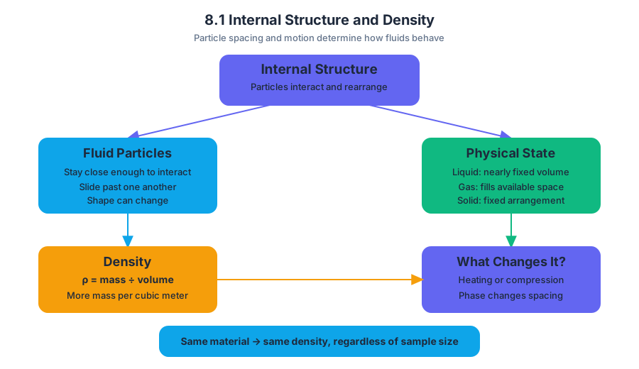
8.2 Pressure
A sharp heel can hurt more than a flat shoe even when both support the same person because pressure depends on how much area receives a force.
8.2 Pressure
A sharp heel can hurt more than a flat shoe even when both support the same person because pressure depends on how much area receives a force. Pressure is the perpendicular force distributed over an area:
$$ P=\frac{F_{\perp}}{A} $$
Here, $P$ is pressure in pascals ($\text{Pa}$), $F_{\perp}$ is the component of force perpendicular to the surface in newtons, and $A$ is the contact area in square meters.
One pascal is one newton per square meter:
$$1\ \text{Pa}=1\ \text{N},\text{m}^{-2}$$
Force and area: the pressure tradeoff
For the same perpendicular force, decreasing area increases pressure. For the same area, increasing force increases pressure. The relationship is proportional in the numerator and inverse in the denominator:
| Change | Effect on pressure |
|---|---|
| Force doubles, area unchanged | Pressure doubles |
| Area doubles, force unchanged | Pressure is halved |
| Force and area both double | Pressure is unchanged |
| Area becomes one-fourth as large | Pressure becomes four times as large |
A $600\ \text{N}$ person stands on two shoes whose combined contact area is $0.040\ \text{m}^2$. The pressure on the floor is
$$ P=\frac{600\ \text{N}}{0.040\ \text{m}^2} =1.5\times10^4\ \text{Pa}. $$
If the person balances on one shoe with area $0.020\ \text{m}^2$, the force is still approximately $600\ \text{N}$, but the pressure becomes
$$ P=\frac{600\ \text{N}}{0.020\ \text{m}^2} =3.0\times10^4\ \text{Pa}. $$
The person has not become heavier; the same force is concentrated over half the area.
Misconception check: pressure is not force
A large force does not automatically mean a large pressure. A snowshoe can support a person with substantial downward force while reducing pressure on the snow because its large area spreads that force. Also, only the force component perpendicular to the surface contributes to the pressure in $P=F_{\perp}/A$; a force directed entirely along the surface does not compress it.
Pressure inside a fluid
A fluid—a liquid or gas—cannot maintain a fixed shape, so it presses on the walls and surfaces that contain it. At rest, fluid pressure acts perpendicular to any surface. Unlike a single contact force, pressure in a fluid is a scalar quantity: at a particular point, it does not have a separate “leftward” or “rightward” value.
In a fluid at rest, pressure increases with depth because deeper fluid must support the weight of the fluid above it. For a liquid of uniform density $\rho$, the pressure at depth $h$ is
$$ P=P_0+\rho gh, $$
where $P_0$ is the pressure at the fluid’s surface, $\rho$ is fluid density, $g$ is gravitational-field strength, and $h$ is vertical depth below the surface.
The term $\rho gh$ is the pressure increase caused by the liquid column. It depends on depth and density, not on the container’s shape. A narrow tube and a wide tank can produce the same pressure at the same depth if they contain the same fluid and have the same surface pressure.
Worked example: pressure below a lake surface
A diver is $5.0\ \text{m}$ below the surface of freshwater. Take $\rho=1.0\times10^3\ \text{kg},\text{m}^{-3}$, $g=9.8\ \text{m},\text{s}^{-2}$, and atmospheric pressure $P_0=1.0\times10^5\ \text{Pa}$. The water’s contribution is
$$ \rho gh
(1.0\times10^3)(9.8)(5.0)
4.9\times10^4\ \text{Pa}. $$
Therefore the total, or absolute, pressure is
$$ P
1.0\times10^5+4.9\times10^4
1.49\times10^5\ \text{Pa}. $$
The pressure increase relative to the surface is $4.9\times10^4\ \text{Pa}$. This is called gauge pressure:
$$ P_{\text{gauge}}=\rho gh. $$
Misconception check: deeper does not mean “more force in every direction”
Greater depth means greater pressure at a point, not a one-way downward push. The fluid exerts pressure on the diver from all directions. The net force becomes upward when the pressure on the diver’s bottom surfaces exceeds the pressure on the top surfaces; that force is the subject of buoyancy in the next dynamics treatment.
A visual way to reason about pressure
When solving a pressure problem, identify three things before calculating:
- The surface: What area receives the force?
- The perpendicular force: Which component is normal to that surface?
- The pressure reference: Is the problem asking for gauge pressure, $\rho gh$, or absolute pressure, $P_0+\rho gh$?
These choices exercise Science Practice 1: Creating Representations when a situation is translated into a force-area diagram or depth model, and Science Practice 2: Mathematical Routines when proportional relationships and units are used consistently. A pressure investigation also uses Science Practice 3: Scientific Questioning and Argumentation when measurements of depth and pressure are used to support or challenge the model $P=P_0+\rho gh$.
Retrieval check
A liquid’s density doubles while the depth and surface pressure remain unchanged. Does the gauge pressure double? Yes, because $P_{\text{gauge}}=\rho gh$ and only $\rho$ changed. Does the absolute pressure necessarily double? No: absolute pressure includes the unchanged surface pressure, so it becomes $P_0+2\rho gh$, not $2(P_0+\rho gh)$.
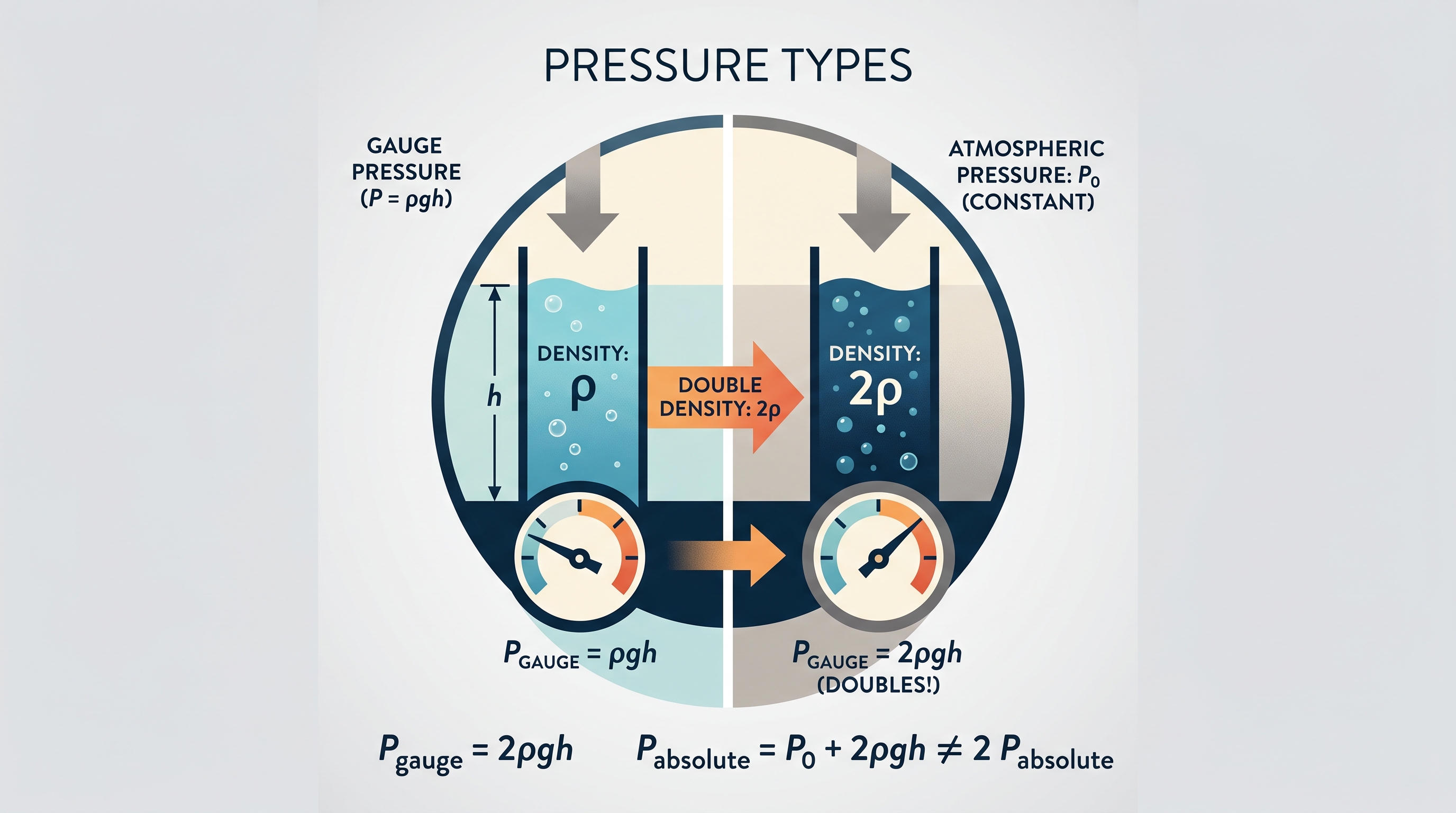
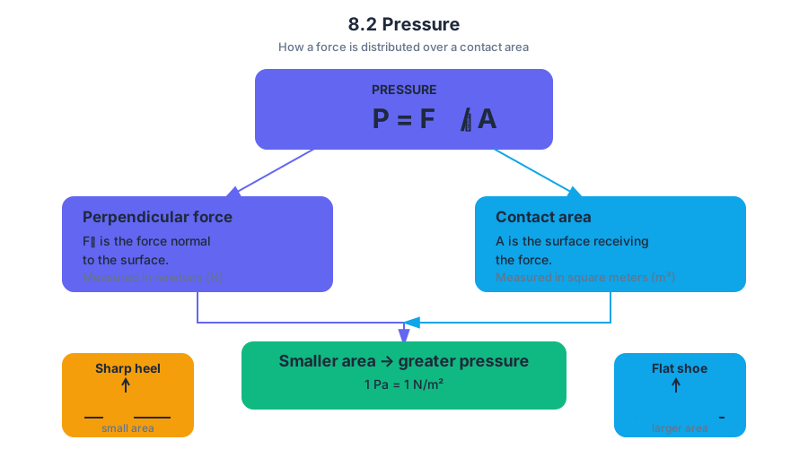
8.3 Fluids and Newton’s Laws
Key concepts: Pressure as force per unit area · Fluid pressure in a column · Dependence of fluid pressure on depth · Dependence of fluid pressure on density · Absolute (total) pressure versus pressure due to the fluid alone · Applying Newton’s laws to fluids · Using experimental data as evidence for a claim · Creating and interpreting graphs with appropriate scales and units · Deriving symbolic expressions from known quantities · Designing experimental procedures and comparing physical quantities
Pressure forces on a fluid surface can produce a net force, and that net force determines whether a fluid element accelerates, remains at rest, or pushes another object upward.
8.3 Fluids and Newton’s Laws
Pressure forces on a fluid surface can produce a net force, and that net force determines whether a fluid element accelerates, remains at rest, or pushes another object upward.
From pressure to net force
Pressure is already defined as perpendicular force per unit area, $P = F_{\perp}/A$. For a fluid element, the important question is not merely the pressure at one location, but whether pressures on opposite surfaces are equal. If the pressure force on one side is larger than the force on the other, the difference is a net force.
Consider a thin horizontal slab of fluid with top and bottom area $A$. If the pressure at the bottom is $P_{\text{bottom}}$ and the pressure at the top is $P_{\text{top}}$, the upward and downward pressure forces are
$$F_{\text{bottom}} = P_{\text{bottom}}A$$
and
$$F_{\text{top}} = P_{\text{top}}A.$$
The slab also has weight $mg$ downward. Newton’s second law gives
$$P_{\text{bottom}}A - P_{\text{top}}A - mg = ma_y.$$
For a stationary fluid element, $a_y=0$, so the pressure difference supports the element’s weight.
Why pressure increases with depth
The mass of a fluid slab with density $\rho$, area $A$, and height $h$ is $m=\rho Ah$. Substituting this into the equilibrium equation gives
$$P_{\text{bottom}}A-P_{\text{top}}A-\rho Ahg=0.$$
Dividing by $A$ produces
$$P_{\text{bottom}}-P_{\text{top}}=\rho gh.$$
Thus, the pressure increase through a vertical fluid column depends on the fluid’s density, gravitational field strength, and depth difference—not on the container’s shape.
The pressure caused by the fluid column alone is called gauge pressure:
$$P_{\text{gauge}}=\rho gh.$$
If the fluid’s upper surface is exposed to the atmosphere, the total, or absolute, pressure at depth $h$ is
$$P_{\text{abs}}=P_{\text{atm}}+\rho gh.$$
The atmospheric term is not produced by the added fluid column; it is the reference pressure already acting at the surface.
Misconception check — “More fluid means more pressure.” A wide, shallow container can hold more water than a narrow, deep container while producing less pressure at its bottom. At the same depth in the same fluid, pressure is the same because $\rho$, $g$, and $h$ are the same. The bottom force can still differ because $F=PA$ and the bottom areas differ.
Worked example: comparing fluids
A sensor is placed $0.80\ \text{m}$ below the surface in freshwater with $\rho_{\text{fresh}}=1.00\times10^3\ \text{kg},\text{m}^{-3}$ and in saltwater with $\rho_{\text{salt}}=1.10\times10^3\ \text{kg},\text{m}^{-3}$. Using $g=9.8\ \text{m},\text{s}^{-2}$,
$$P_{\text{gauge,fresh}}=(1.00\times10^3)(9.8)(0.80)=7.84\times10^3\ \text{Pa},$$
while
$$P_{\text{gauge,salt}}=(1.10\times10^3)(9.8)(0.80)=8.62\times10^3\ \text{Pa}.$$
The atmospheric pressure is added to both values when absolute pressure is requested, so the difference between the two absolute pressures is still $7.84\times10^2\ \text{Pa}$.
Newton’s laws in fluids
Pressure differences explain buoyant forces. The lower surface of a submerged object is deeper than its upper surface, so the upward pressure force is larger than the downward pressure force. The resulting net force is the buoyant force, directed upward. Newton’s second law then determines the object’s motion:
$$F_{\text{net},y}=F_B-mg=ma_y.$$
In a denser fluid, the same displaced volume produces a larger pressure difference and therefore a larger buoyant force, since $F_B=\rho_{\text{fluid}}V_{\text{displaced}}g$.
Skill connection: 1.A: Create diagrams, tables, charts, or schematics to represent physical situations is used in pressure-column and force diagrams. 2.A: Derive a symbolic expression from known quantities by selecting and following a logical mathematical pathway appears in the derivation of $\Delta P=\rho gh$. 2.D: Predict new values or factors of change of physical quantities using functional dependence between variables supports predictions such as “doubling depth doubles gauge pressure.” 1.B: Create quantitative graphs with appropriate scales and units, including plotting data applies when graphing pressure versus depth. A linear graph has slope
$$\frac{\Delta P}{\Delta h}=\rho g.$$
For an investigation, measure pressure at several known depths while keeping the fluid and sensor orientation fixed. Plot $P_{\text{gauge}}$ on the vertical axis in pascals and $h$ on the horizontal axis in meters; a best-fit line should pass near the origin, and its slope can be divided by $g$ to determine $\rho$. A strong procedure also repeats measurements, controls temperature and fluid composition, and justifies uncertainty reduction.
2.C: Compare physical quantities between two or more scenarios or at different times and locations in a single scenario asks for more than a numerical difference: identify which variable changed and use the model to explain the direction of change. 3.A: Create experimental procedures that are appropriate for a given scientific question and 3.B: Apply an appropriate law, definition, theoretical relationship, or model to make a claim connect measurements to Newton’s laws and the pressure model.
Retrieval check: At equal depth, which produces greater gauge pressure: freshwater or saltwater? If a submerged object has $F_B>mg$, what does Newton’s second law predict about its vertical acceleration?
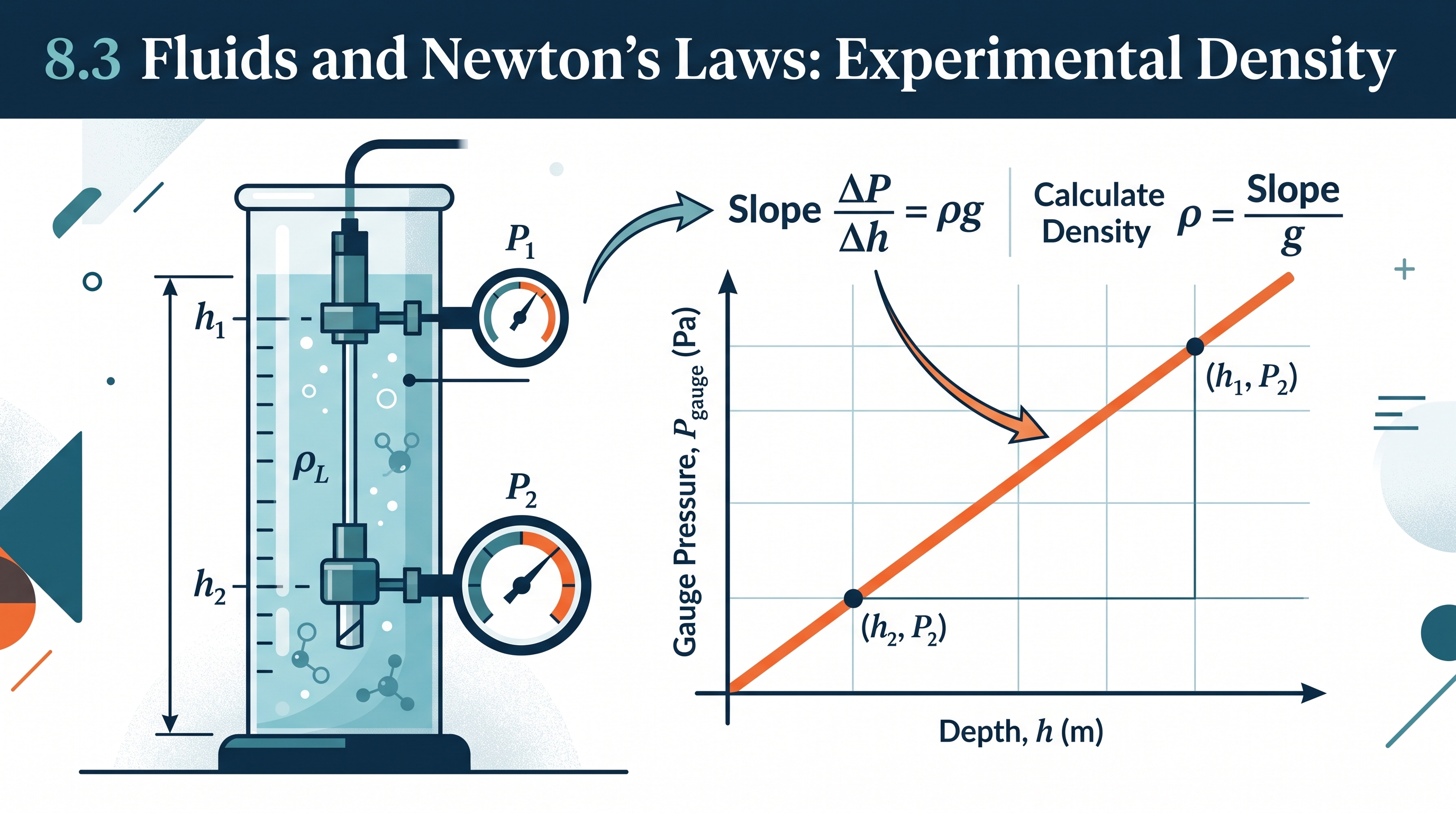
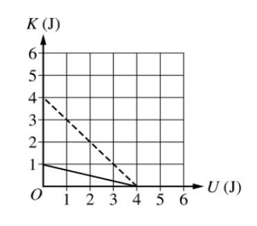
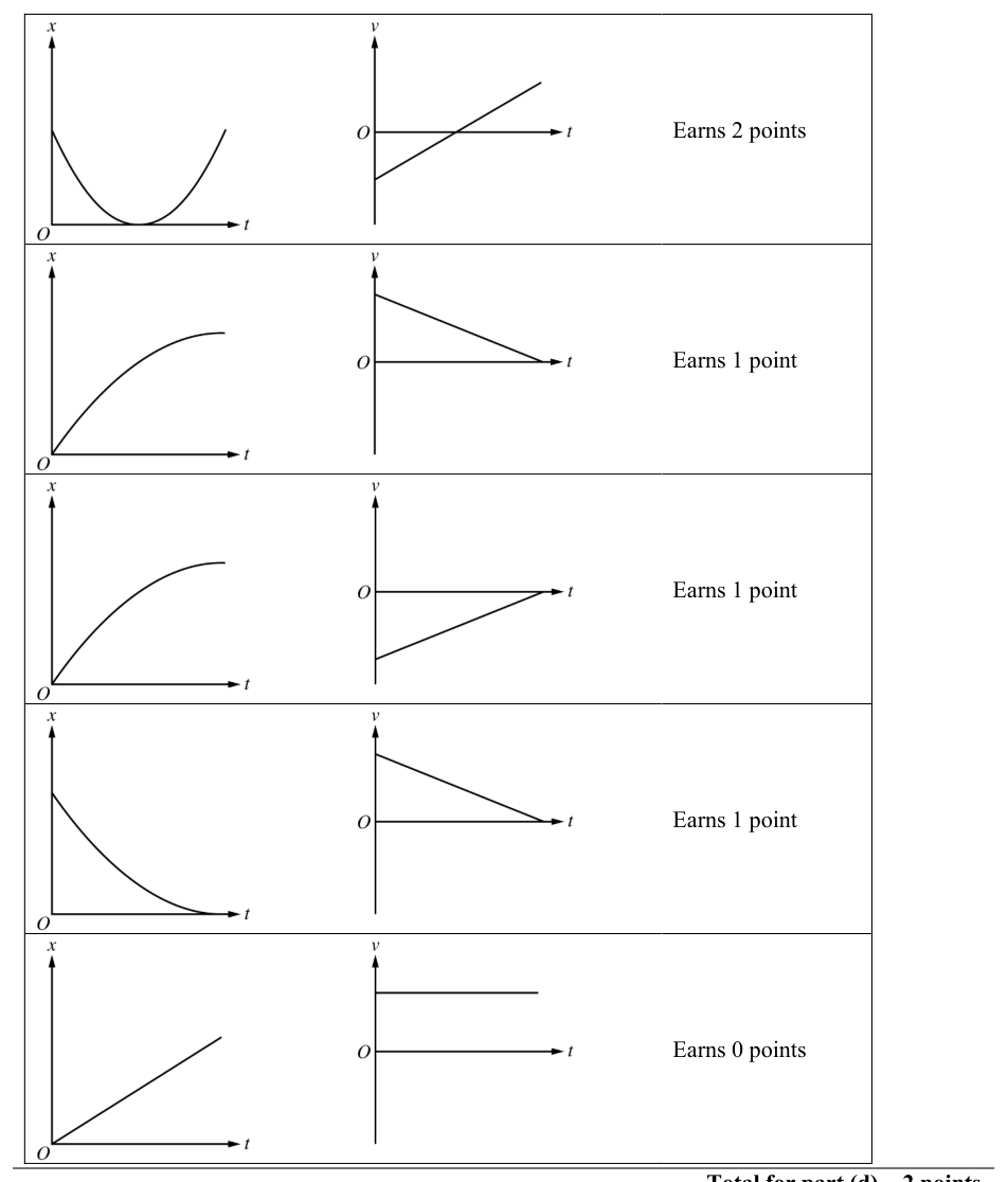
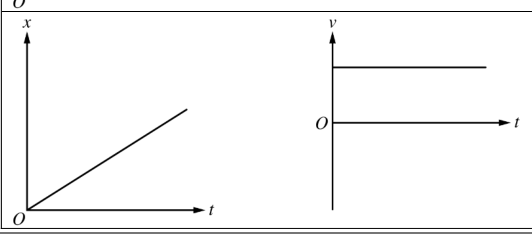
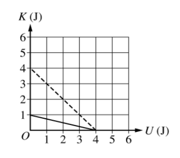
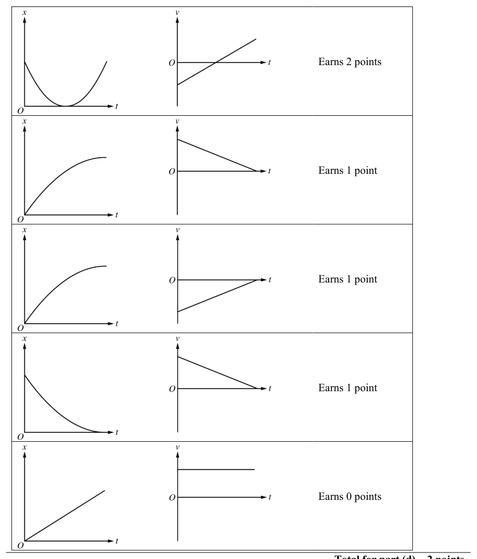
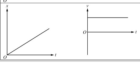
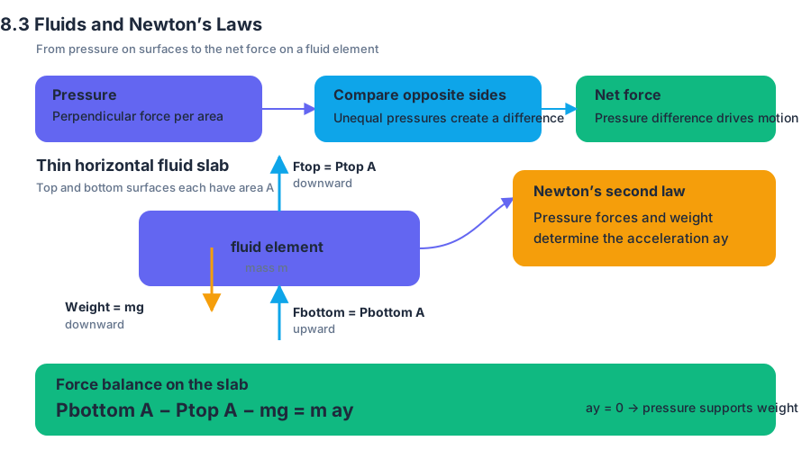
8.4 Fluids and Conservation Laws
Key concepts: Conservation of mass flow rate in incompressible fluids · Fluid–Earth system energy differences · Gravitational potential energy differences between locations · Functional dependence between physical variables · Applying laws, definitions, theoretical relationships, or models · Predicting changes in physical quantities · Representing data with appropriate scales and units · Plotting and interpreting data
A narrow section of pipe can make water move faster without creating extra water: when an incompressible fluid enters a region, the same mass flow rate must leave it.
8.4 Fluids and Conservation Laws
A narrow section of pipe can make water move faster without creating extra water: when an incompressible fluid enters a region, the same mass flow rate must leave it. Conservation laws connect that flow constraint to changes in pressure, speed, and gravitational potential energy.
Conservation of mass flow rate
Mass flow rate is the mass passing a cross section per unit time. For an incompressible fluid flowing steadily through a tube, the flow rate is conserved. The relevant continuity relationship is
$$ A_1v_1=A_2v_2 $$
where $A$ is cross-sectional area and $v$ is the fluid speed perpendicular to that area.
If a pipe narrows so that $A_2=\frac{1}{4}A_1$, then
$$ A_1v_1=\frac{1}{4}A_1v_2 \qquad\Rightarrow\qquad v_2=4v_1. $$
The fluid moves four times faster in the narrow section. The equation does not say that speed is always constant; it says that area and speed adjust so the same amount of incompressible fluid passes each location.
This is the required idea in 8.4.A.2, supported by 8.4.A.1.i: in a fluid-filled tube open at both ends, the rate at which matter enters must equal the rate at which matter exits. A pressure difference can cause the fluid to flow, as stated in 8.4.A.1, but once steady flow is established, continuity determines how speed changes from place to place.
Energy differences in the fluid–Earth system
A fluid–Earth system can store energy in several forms. For a fluid element of mass $m$, gravitational potential energy is
$$ U_g=mgy, $$
so the difference between two locations is
$$ \Delta U_g=mg(y_2-y_1). $$
A higher location has greater gravitational potential energy when $g$ is approximately constant. Per unit volume, the corresponding energy difference is $\rho g(y_2-y_1)$, where $\rho$ is fluid density.
For steady, incompressible, nonviscous flow along a streamline, conservation of mechanical energy is expressed by Bernoulli’s equation:
$$ P_1+\frac{1}{2}\rho v_1^2+\rho gy_1
P_2+\frac{1}{2}\rho v_2^2+\rho gy_2. $$
Here $P$ is pressure energy per unit volume, $\frac{1}{2}\rho v^2$ is kinetic energy per unit volume, and $\rho gy$ is gravitational potential energy per unit volume. If viscosity or turbulence converts mechanical energy into thermal energy, this ideal relationship must be modified; it should not be applied automatically.
Worked comparison: a narrowing, rising pipe
Water flows from location $1$ to location $2$. Let $\rho=1000\ \mathrm{kg/m^3}$, $v_1=1.0\ \mathrm{m/s}$, $A_2=\frac14A_1$, and $y_2=y_1+2.0\ \mathrm{m}$. Suppose $P_1=1.50\times10^5\ \mathrm{Pa}$.
First use continuity:
$$ v_2=\frac{A_1}{A_2}v_1=4(1.0)=4.0\ \mathrm{m/s}. $$
The kinetic-energy density increases by
$$ \Delta\left(\frac12\rho v^2\right)
\frac12(1000)\left(4.0^2-1.0^2\right)
7500\ \mathrm{Pa}. $$
The gravitational-potential-energy density increases by
$$ \rho g\Delta y=(1000)(9.8)(2.0)=19600\ \mathrm{Pa}. $$
Bernoulli’s equation gives
$$ P_2=P_1+\frac12\rho(v_1^2-v_2^2)+\rho g(y_1-y_2), $$
so
$$ P_2
150000-7500-19600
122900\ \mathrm{Pa}. $$
The fluid gains energy density because it rises and speeds up. That energy comes from a decrease in pressure energy: $P_2<P_1$. A narrower pipe alone would tend to lower pressure as speed increases; raising the pipe creates an additional pressure decrease because the fluid also gains gravitational potential energy.
Using functional dependence to predict changes
Skill 2.D — Predict new values or factors of change of physical quantities using functional dependence between variables is especially powerful here. From continuity, $v\propto A^{-1}$: halving area doubles speed. From gravitational potential energy, $U_g\propto m$, $U_g\propto g$, and $U_g\propto y$, so doubling the height difference doubles the gravitational-energy difference when the other quantities remain fixed.
The topic also develops 2.A — Derive a symbolic expression from known quantities by selecting and following a logical mathematical pathway, 2.C — Compare physical quantities between two or more scenarios or at different times and locations in a single scenario, and 3.B — Apply an appropriate law, definition, theoretical relationship, or model to make a claim. A strong response identifies the system, states assumptions, writes continuity or Bernoulli’s equation, and then interprets the sign and factor of change.
Data, procedures, and common traps
For an investigation, 3.A — Create experimental procedures that are appropriate for a given scientific question might require measuring tube diameter, timing a known volume of collected fluid, and repeating measurements at several locations or flow rates. Under 1.B — Create quantitative graphs with appropriate scales and units, including plotting data, graph variables that test the model: for example, plot $v$ against $1/A$ to test $v\propto1/A$, label axes with units, and use a scale that displays all measurements clearly.
Misconception check: “Faster fluid always means lower pressure.” Not by itself. Bernoulli’s equation compares all energy terms. A fluid can speed up while moving downward, gaining kinetic energy partly from gravitational potential energy; pressure need not decrease by the same amount, or may even increase depending on the height change and other conditions.
Retrieval check: A pipe’s area decreases by a factor of $3$, and the fluid is incompressible. What happens to its speed? If the pipe then rises, which two terms in Bernoulli’s equation increase, and what must happen to pressure if no other energy source or loss is present?
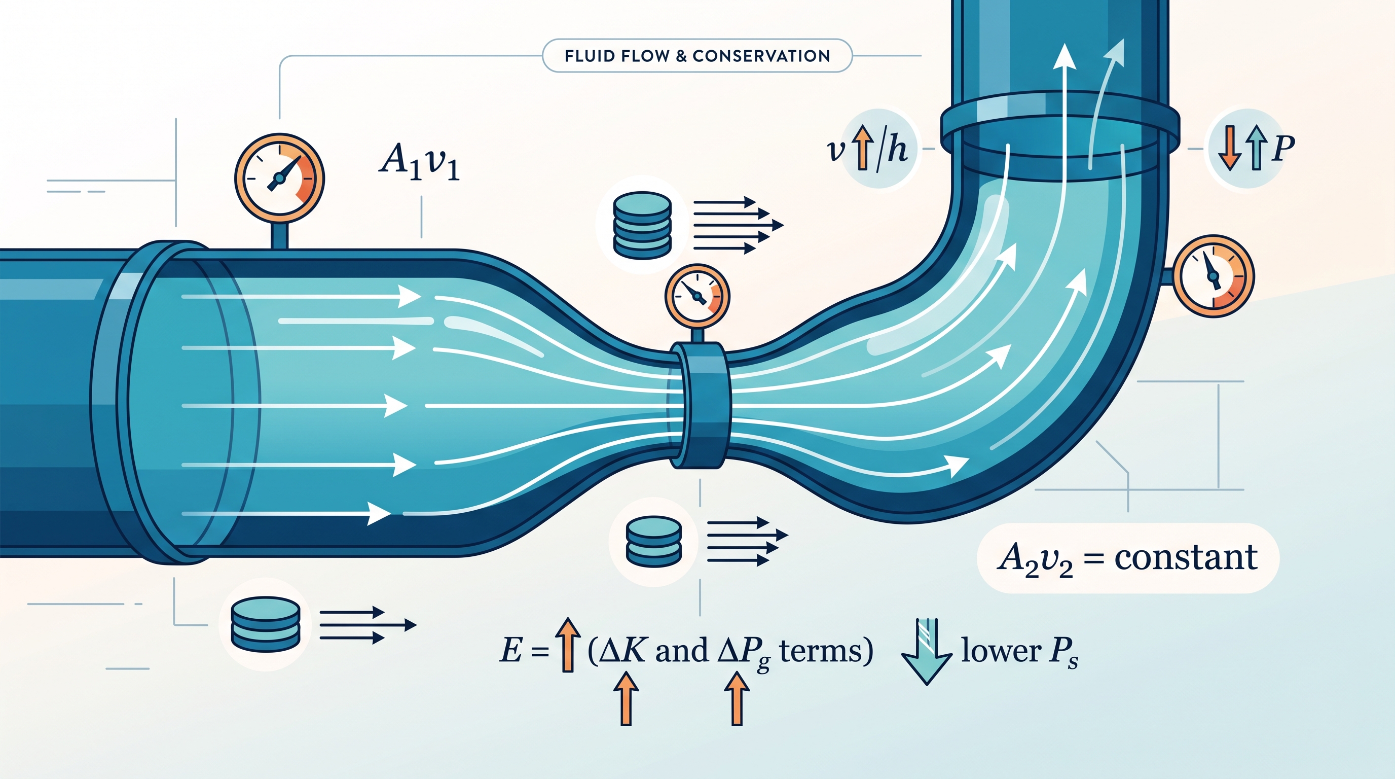
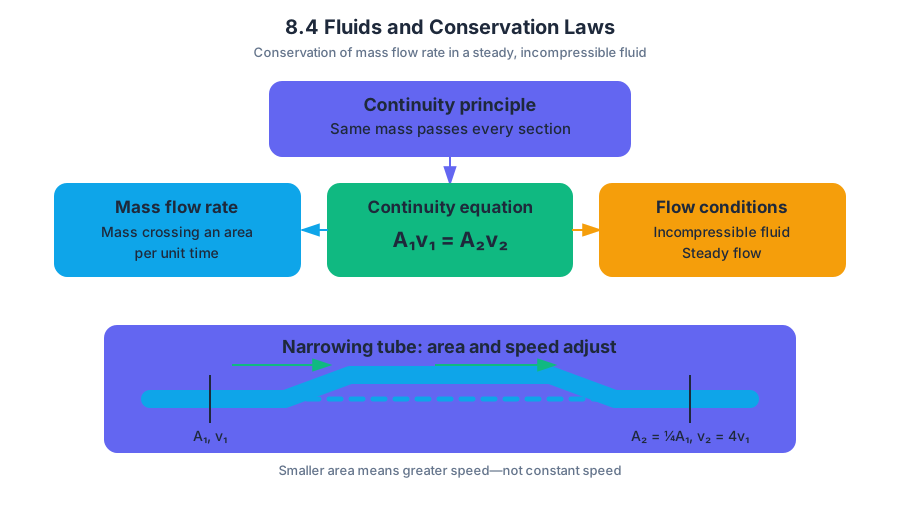
AP Practice 1
Key concepts: AP Physics 1 Algebra-Based course framework effective Fall 2024 · AP course principles: evidence-based reasoning and independent thinking · Respectful debate and inclusion of diverse perspectives in AP classrooms · Multiple-choice exam structure updates · Inquiry-based laboratory instruction · Science practices in AP Physics 1 · Hands-on laboratory work and course time allocation · The eight AP Physics 1 course units · Multiple representations in kinematics · Momentum of rotating systems, oscillations, and fluids
AP Physics 1 is an algebra-based, introductory college-level physics course whose framework is effective beginning in Fall 2024. Its central question is not merely “Which equation applies?” but How can evidence, representations, mathematics, and physical principles justify a claim about what a system does?
AP Practice 1
AP Physics 1 is an algebra-based, introductory college-level physics course whose framework is effective beginning in Fall 2024. Its central question is not merely “Which equation applies?” but How can evidence, representations, mathematics, and physical principles justify a claim about what a system does?
The course as a connected physical story
The framework contains eight units arranged from describing motion to analyzing interactions, conservation laws, rotation, oscillations, and fluids. Their multiple-choice exam weightings are:
| Unit | Multiple-choice exam weighting |
|---|---|
| Unit 1: Kinematics | $10$–$15%$ |
| Unit 2: Force and Translational Dynamics | $18$–$23%$ |
| Unit 3: Work, Energy, and Power | $18$–$23%$ |
| Unit 4: Linear Momentum | $10$–$15%$ |
| Unit 5: Torque and Rotational Dynamics | $10$–$15%$ |
| Unit 6: Energy and Momentum of Rotating Systems | $5$–$8%$ |
| Unit 7: Oscillations | $5$–$8%$ |
| Unit 8: Fluids | $10$–$15%$ |
The sequence is deliberately interconnected. A motion graph from Unit 1 can become evidence for a force model in Unit 2; the same system can then be analyzed using energy in Unit 3 or momentum in Unit 4. Physics becomes more powerful when a student can translate among a diagram, graph, equation, data table, and verbal explanation.
The complete science-practice framework
Creating Representations means building or interpreting a useful model of a physical situation: a motion map, free-body diagram, graph, energy bar chart, vector diagram, or symbolic equation. In Unit 1, for example, a position–time graph and a velocity–time graph represent the same motion differently; the slope of the first gives velocity, while the slope of the second gives acceleration.
Mathematical Routines means using algebraic, proportional, graphical, and computational reasoning to connect quantities. A strong solution does not begin with random substitution. It identifies the relationship, tracks units, rearranges symbolically when useful, and checks whether the result has a physically sensible direction and magnitude.
Scientific Questioning begins with a testable question about a system. Data Analysis then uses measurements, graphs, patterns, uncertainty, and comparisons to evaluate what happened. Theoretical Relationships connect the evidence to principles such as Newton’s laws, conservation of energy, or momentum. Argumentation completes the chain: a claim is supported by relevant evidence and justified through an appropriate physical relationship.
These practices appear both in laboratories and on the exam. A laboratory may ask students to design a procedure and defend a conclusion from data; a free-response problem may ask them to interpret a graph, derive a relationship, justify an experimental choice, or explain why a prediction agrees or disagrees with observations. Multiple-choice questions can test the same practices more briefly through a diagram, data set, graph, or claim.
Inquiry laboratory work
At least $25%$ of instructional time must involve hands-on laboratory work, and those laboratories should emphasize inquiry rather than following a recipe with predetermined results. Inquiry-based investigation gives students room to pose a question, choose measurements, identify variables, construct representations, analyze data, and defend a conclusion.
A simple motion investigation illustrates the idea. Students could measure a rock’s position with a stopwatch, or record a cart moving along a track. Tilting the track slightly provides approximately constant acceleration in either direction. Students might ask how position changes with time, collect repeated measurements, graph the results, and decide whether the data support a constant-acceleration model.
The important product is not just a numerical value for acceleration. It is an evidence-based argument: the measured pattern supports or does not support the proposed model because the graph, calculated quantities, and uncertainties show a particular relationship. Lab notebooks or portfolios preserve this reasoning.
Evidence, independence, and inclusion
AP classrooms are expected to encourage evidence-based reasoning and independent thinking. Students should evaluate arguments, not one another. Respectful disagreement is productive when it focuses on the model, evidence, assumptions, or logic rather than on a person.
Inclusion does not require students to adopt one cultural or political viewpoint. AP students are not expected to subscribe to one specific set of cultural or political values; they are expected to engage seriously with physical evidence and explain their reasoning clearly while respecting diverse perspectives.
Multiple-choice update and practice
Beginning with the May 2027 AP Physics 1 exam, the multiple-choice section changes from $40$ to $42$ questions, and its allotted time increases from the previous $80$ minutes. The practical consequence is still the same: use representations and proportional reasoning early, avoid becoming trapped in lengthy algebra, and return later to unusually time-consuming questions.
Original multiple-choice practice: A cart moves along a slightly tilted track. Its velocity changes from $+0.40\ \mathrm{m/s}$ to $+1.60\ \mathrm{m/s}$ during a $3.0\ \mathrm{s}$ interval. Which statement is necessarily supported by these measurements?
A. The cart’s acceleration is zero.
B. The cart travels in the negative direction.
C. The cart has a positive average acceleration.
D. The cart’s position remains constant.
Answer: C. Apply the definition of average acceleration:
$$ a_{\mathrm{avg}}=\frac{\Delta v}{\Delta t} =\frac{1.60-0.40}{3.0} =+0.40\ \mathrm{m/s^2}. $$
The positive sign establishes positive average acceleration. It does not by itself prove constant acceleration, and positive acceleration is not the same as positive velocity at every instant.
For a $42$-question section, a useful first-pass rhythm is roughly $2$ minutes per question, while preserving time to revisit marked items. After practice, classify each error as a representation error, mathematical-routine error, data-analysis error, theoretical-relationship error, or argumentation error; correcting the category is more valuable than merely memorizing the answer.

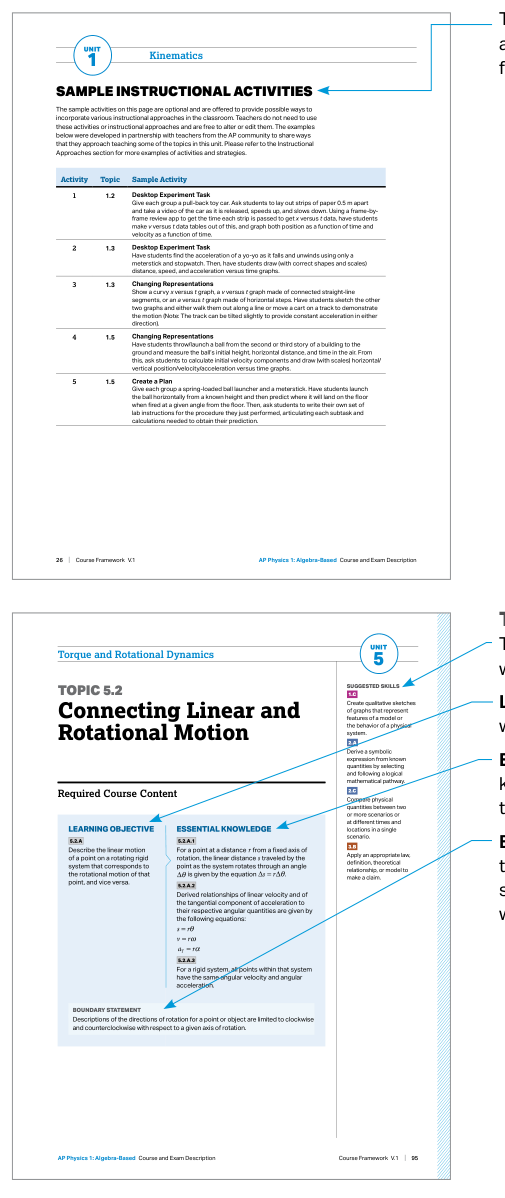
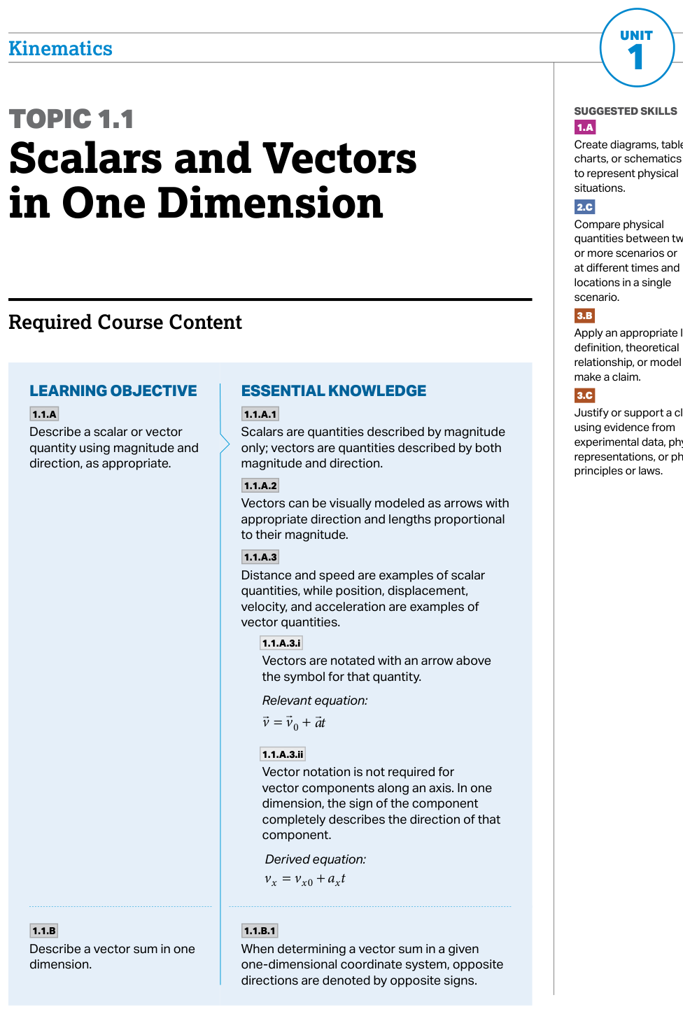
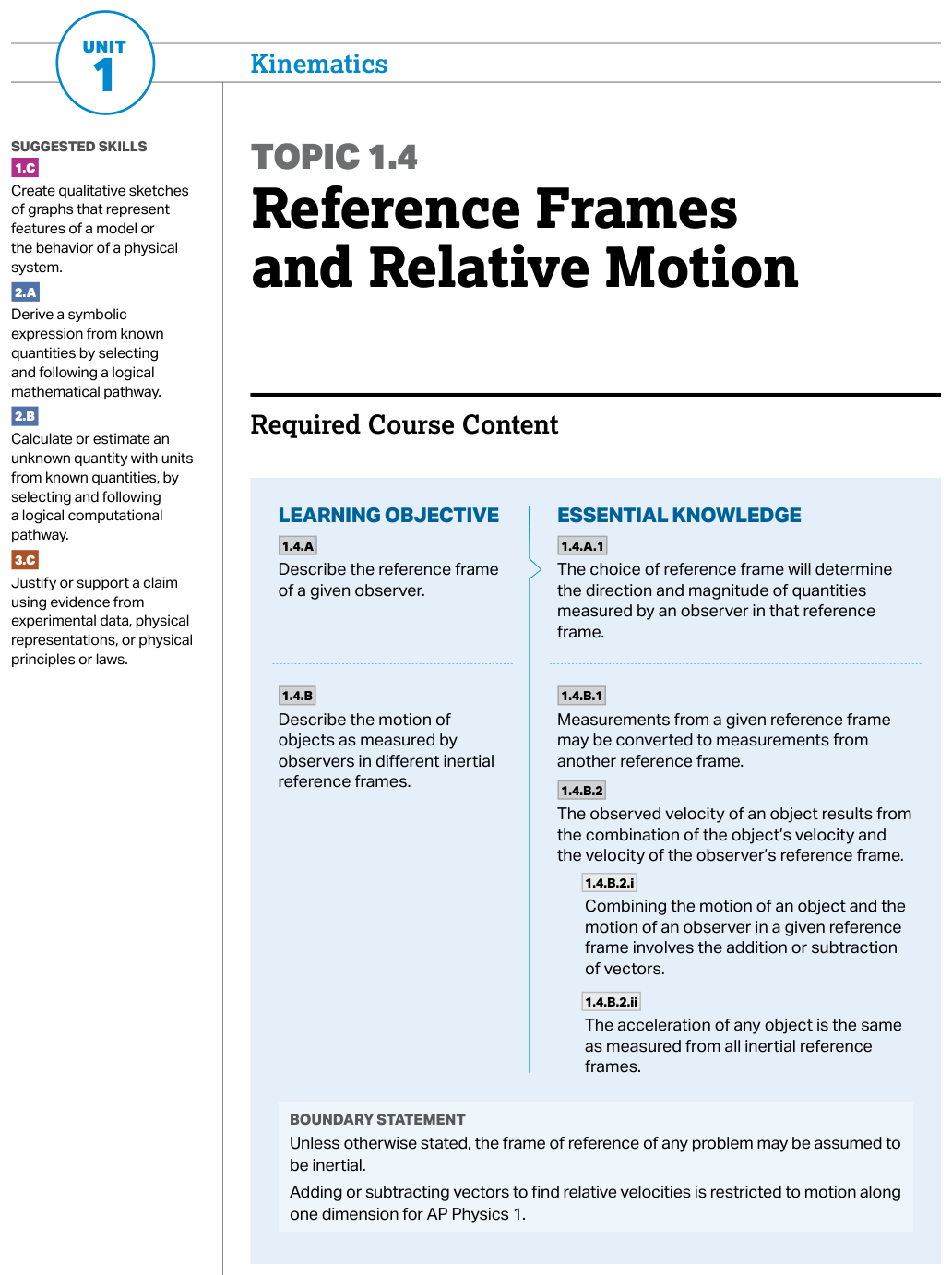
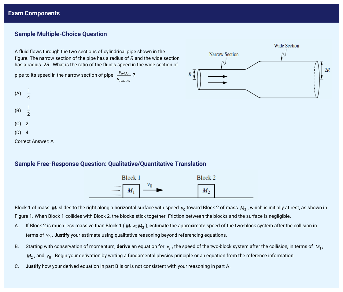


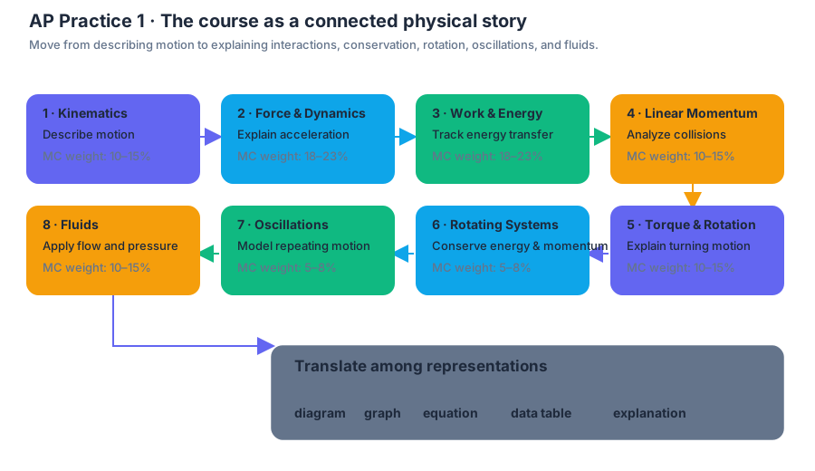
AP Practice 2
Key concepts: AP Physics exam structure and timing · Position-time and velocity-time representations · Newton’s second law and system analysis · Static friction and coefficient of friction · Kinetic (sliding) friction · Circular motion and centripetal acceleration · Tangential and net acceleration · Tension in strings with nonnegligible mass · Gravitational field near Earth’s surface · Motion and force modeling using equations and narratives
A motion graph is not merely a picture of motion: its slope, curvature, and changing direction make testable claims about velocity, acceleration, and force. A strong multiple-choice solution moves through a chain:
AP Practice 2
A motion graph is not merely a picture of motion: its slope, curvature, and changing direction make testable claims about velocity, acceleration, and force. A strong multiple-choice solution moves through a chain:
$$ \text{representation} \rightarrow \text{physical model} \rightarrow \text{equation} \rightarrow \text{claim} $$
The AP Physics 1 exam lasts $180\ \text{min}$. Beginning with the updated format, $5\ \text{min}$ are shifted from free response to multiple choice to accommodate two additional multiple-choice questions. Use this practice as a rapid mixed set: aim for about $2\ \text{min}$ per question, but reserve the final minutes to check units, signs, and whether your selected model matches the physical situation.
Question 1: Frame-by-frame motion
A camera records a cart moving along a straight track. The cart’s position is measured every $1.0\ \text{s}$:
| Time $t$ ($\text{s}$) | Position $x$ ($\text{m}$) |
|---|---|
| $0$ | $0$ |
| $1$ | $1$ |
| $2$ | $4$ |
| $3$ | $9$ |
Which description best matches the cart’s motion?
(A) Constant positive velocity
(B) Constant positive acceleration
(C) Constant negative acceleration
(D) Positive velocity that is decreasing
Answer: (B). The successive displacements are $1\ \text{m}$, $3\ \text{m}$, and $5\ \text{m}$ during equal time intervals. The displacement increases by equal amounts, so the velocity increases at a constant rate. The position-time data are consistent with
$$x=t^2,$$
which gives
$$v=\frac{dx}{dt}=2t$$
and
$$a=\frac{dv}{dt}=2\ \text{m/s}^2.$$
The crucial correction is that the displacements do not increase by equal amounts; their equal increases indicate constant acceleration. Choice (A) would require equal displacements in equal time intervals, while (D) predicts decreasing displacement.
Question 2: Newton’s second law and systems
A $4.0\ \text{kg}$ box is pulled horizontally by a rope with force $18\ \text{N}$. Kinetic friction opposes the motion with force $6.0\ \text{N}$. What is the box’s acceleration?
(A) $1.5\ \text{m/s}^2$
(B) $3.0\ \text{m/s}^2$
(C) $4.5\ \text{m/s}^2$
(D) $6.0\ \text{m/s}^2$
Answer: (B). Choose the box as the system and calculate the net horizontal force:
$$F_{\text{net}}=18\ \text{N}-6.0\ \text{N}=12\ \text{N}.$$
Newton’s second law gives
$$F_{\text{net}}=ma,$$
so
$$a=\frac{12\ \text{N}}{4.0\ \text{kg}}=3.0\ \text{m/s}^2.$$
This explicitly connects the equation to the physical situation. The unit check is decisive: $\text{N}/\text{kg}=\text{m/s}^2$.
Question 3: Static and kinetic friction
A student gradually increases the pull on a crate using a spring scale. The crate remains at rest until the scale reads $24\ \text{N}$, then begins sliding. While it slides at constant speed, the scale reads $18\ \text{N}$. The normal force is $80\ \text{N}$. Which pair gives the coefficients of friction?
(A) $\mu_s=0.23,\ \mu_k=0.30$
(B) $\mu_s=0.30,\ \mu_k=0.23$
(C) $\mu_s=0.30,\ \mu_k=0.30$
(D) $\mu_s=0.23,\ \mu_k=0.23$
Answer: (B). The largest static friction is the force just before slipping:
$$\mu_s=\frac{f_{s,\max}}{N}=\frac{24\ \text{N}}{80\ \text{N}}=0.30.$$
During sliding at constant speed, the net force is zero, so the kinetic friction equals the pulling force:
$$f_k=18\ \text{N},\qquad \mu_k=\frac{18\ \text{N}}{80\ \text{N}}=0.225\approx0.23.$$
Misconception check: static friction is not always $\mu_sN$; it adjusts up to a maximum. Slipping and sliding occur when the surfaces move relative to one another, so kinetic friction applies after motion begins.
Question 4: Circular motion
A car travels around a circular track. Its speed is increasing. Which statement correctly describes its acceleration?
(A) It points only tangent to the track.
(B) It points only toward the center.
(C) It has a centripetal component toward the center and a tangential component along the track.
(D) It is zero because the car follows a circular path.
Answer: (C). The centripetal acceleration points toward the center:
$$a_c=\frac{v^2}{r}.$$
Because the speed is increasing, the car also has tangential acceleration, directed tangent to the path. The net acceleration is the vector sum:
$$\vec a=\vec a_c+\vec a_t.$$
A changing velocity requires acceleration even if the car’s path is smooth and its speed were constant.
Examiner-reward reasoning and error review
For multiple choice, the scored result is the selected answer, but the physics behind it should still satisfy Science Practice 1: Creating Representations, Science Practice 2: Mathematical Routines, and Science Practice 3: Scientific Questioning and Argumentation. In particular, 2.A: Deriving new expressions from fundamental principles supports using $F_{\text{net}}=ma$ and friction definitions; 2.D: Making predictions using functional dependence between variables supports reading how $x$, $v$, and $a$ change; 3.B: Making claims supports selecting the motion description; and 3.C: Supporting claims using evidence supports citing slopes, force differences, and acceleration components.
After checking your answers, classify every error: representation error, model-selection error, algebra or arithmetic error, unit error, or misconception. Re-solve without looking at the answer, then write one sentence of evidence—for example, “The increasing successive displacements show increasing velocity, not constant velocity.” That sentence turns a guessed choice into a defensible physical claim.

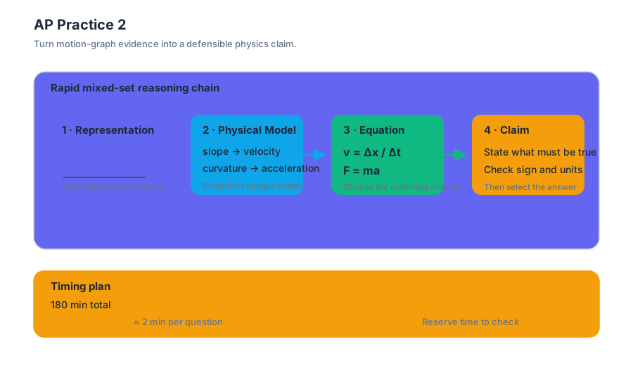
AP Practice 3
A strong physics investigation does more than produce a number: it connects a question, a controlled procedure, measured data, a mathematical model, and an evidence-based claim.
AP Practice 3
A strong physics investigation does more than produce a number: it connects a question, a controlled procedure, measured data, a mathematical model, and an evidence-based claim. This practice focuses on the free-response task type that asks you to design or analyze an experiment and defend a conclusion using representations, mathematical routines, and scientific argumentation.
Timing target: spend approximately $12$–$15$ minutes on one experimental-design or data-analysis task. Do not begin by calculating. First identify the physical relationship being tested, the variables that must be controlled, and the representation that will make the model visible.
The original investigation task
A student investigates how the period $T$ of a small-angle pendulum depends on its length $L$. The student has a pendulum, a meterstick, a stopwatch, and a digital balance. The pendulum bob is released from the same small angle for every trial.
The student measures the following values:
| $L$ (m) | $T$ (s) |
|---|---|
| $0.25$ | $1.00$ |
| $0.40$ | $1.27$ |
| $0.60$ | $1.56$ |
| $0.90$ | $1.91$ |
| $1.20$ | $2.20$ |
Task.
- Design a graph that can test whether the model $T \propto \sqrt{L}$ is supported.
- Describe one important procedure for reducing uncertainty in the period measurement.
- Use the data to determine whether the model is reasonable.
- Explain why the bob’s mass does not appear in the proposed model.
Step 1: Choose a representation that tests the model
The statement $T \propto \sqrt{L}$ is not tested most directly by plotting $T$ versus $L$. Instead, define a transformed variable:
$$ x=\sqrt{L} $$
If the model is correct, then
$$ T=k\sqrt{L} $$
where $k$ is a constant. Therefore, a graph of $T$ on the vertical axis versus $\sqrt{L}$ on the horizontal axis should be approximately linear and should pass near the origin.
This response demonstrates Science Practice 1: Creating Representations, especially 1.B. Create quantitative graphs with appropriate scales and units, including plotting data, and 1.C. Create qualitative sketches of graphs that represent features of a model or the behavior of a physical system. A complete graph needs labeled axes, units, sensible scaling, plotted points, and a line or curve that represents the trend.
For the data, the transformed values are approximately:
| $L$ (m) | $\sqrt{L}$ ($\text{m}^{1/2}$) | $T$ (s) |
|---|---|---|
| $0.25$ | $0.50$ | $1.00$ |
| $0.40$ | $0.63$ | $1.27$ |
| $0.60$ | $0.77$ | $1.56$ |
| $0.90$ | $0.95$ | $1.91$ |
| $1.20$ | $1.10$ | $2.20$ |
Step 2: Improve the measurement
A single stopwatch measurement includes the student’s reaction time when starting and stopping the timer. A better procedure is to measure the time for many complete oscillations, such as $10$ or $20$, and divide by the number of oscillations:
$$ T=\frac{t_{\text{total}}}{N} $$
Repeating this process and averaging the results further reduces the effect of random timing uncertainty. This is an example of Science Practice 3: Scientific Questioning & Argumentation, because the procedure is justified by the type of evidence needed to answer the question.
Step 3: Use the model to interpret the data
The transformed data give nearly constant values of $T/\sqrt{L}$:
$$ \frac{1.00}{0.50}=2.00\ \text{s},\text{m}^{-1/2} $$
$$ \frac{2.20}{1.10}=2.00\ \text{s},\text{m}^{-1/2} $$
The intermediate points produce values close to $2.00\ \text{s},\text{m}^{-1/2}$ as well. Thus, the graph of $T$ versus $\sqrt{L}$ would be approximately linear, supporting the model within experimental uncertainty.
This uses Science Practice 2: Mathematical Routines, specifically 2.A. Derive a symbolic expression from known quantities by selecting and following a logical mathematical pathway, 2.B. Calculate or estimate an unknown quantity with units from known quantities, by selecting and following a logical computational pathway, and 2.C. Compare physical quantities between two or more scenarios or at different times and locations in a single scenario.
Step 4: Explain the missing mass
For a small-angle pendulum, the period is modeled by
$$ T=2\pi\sqrt{\frac{L}{g}} $$
The bob’s mass does not appear because the gravitational force and the bob’s inertia both increase in proportion to mass. Their effects cancel in the equation of motion. A heavier bob may have a different air-resistance behavior, but in the ideal model its mass does not change the period.
Examiner-rewarded reasoning: identify the transformed graph, include units and scales, propose a procedure linked to uncertainty reduction, use data to support or reject the model, and justify the absence of mass from the governing relationship.
Named misconception — “More mass means a faster pendulum.” Mass can change the forces involved, but it also changes the inertia resisting acceleration by the same factor. For the ideal pendulum model, length and gravitational acceleration determine the period.
Error-review routine: after solving, check four items: Did the graph test the stated proportionality? Did the procedure control relevant variables? Did the conclusion cite data rather than merely assert agreement? Did every calculated quantity carry appropriate units?
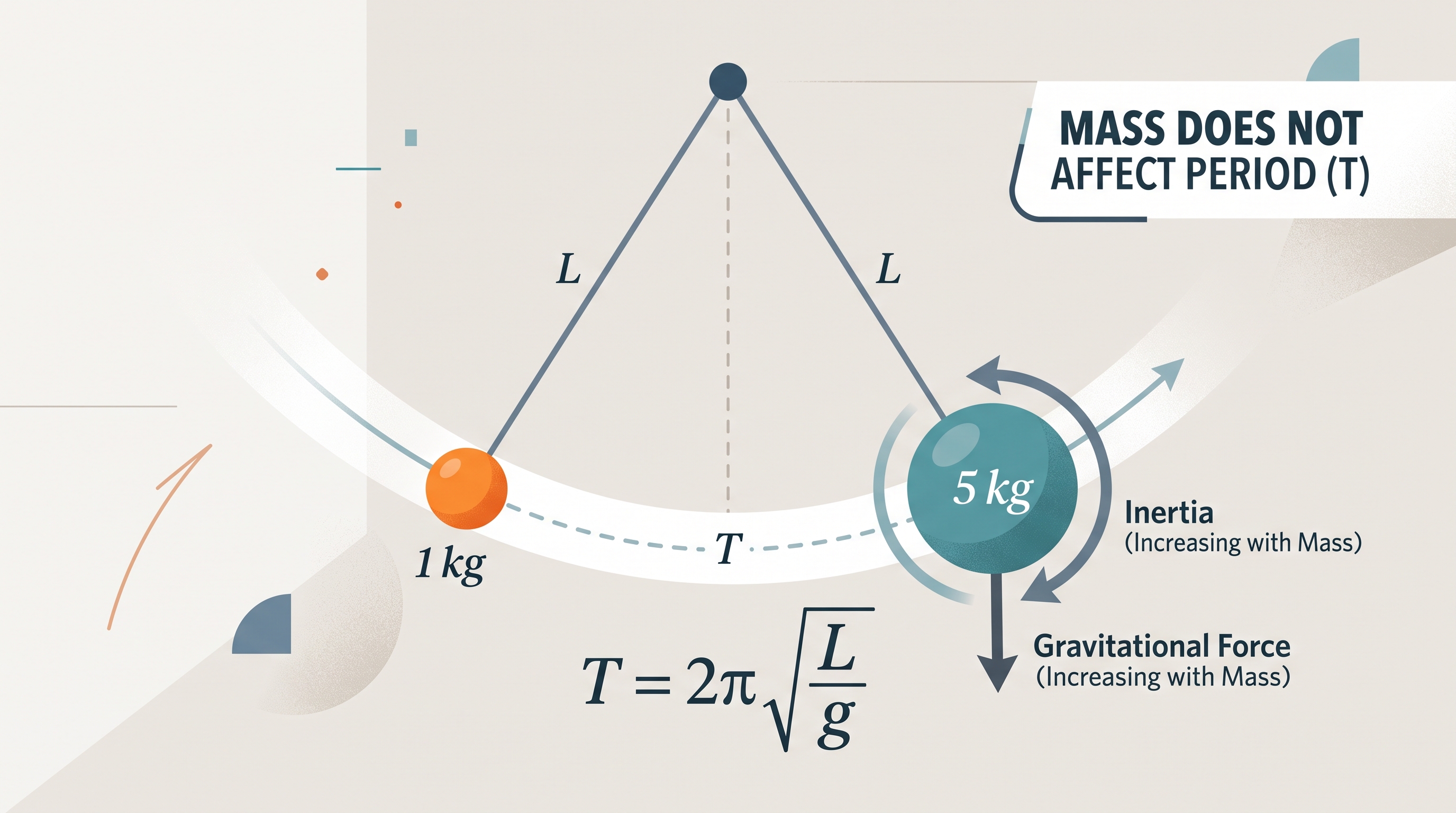
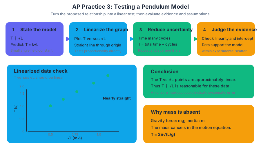
AP Practice 4
A strong experimental-design response does more than name an equation: it turns a physical question into measurable variables, a controlled procedure, evidence-based analysis, and a defensible claim.
AP Practice 4
A strong experimental-design response does more than name an equation: it turns a physical question into measurable variables, a controlled procedure, evidence-based analysis, and a defensible claim. In AP Physics 1, this task type especially exercises Science Practice 1: Creating Representations, Science Practice 2: Mathematical Routines, and Science Practice 3: Scientific Questioning & Argumentation.
The task type: experimental design and analysis
Treat the prompt as an investigation pipeline:
$$ \text{question} \longrightarrow \text{model} \longrightarrow \text{variables} \longrightarrow \text{procedure} \longrightarrow \text{data representation} \longrightarrow \text{claim} $$
The scoring opportunity is usually distributed across several kinds of reasoning: creating a useful diagram or graph, selecting measurable quantities, controlling variables, using mathematics consistently, and connecting the evidence to a physical principle. A response can lose credit even when its final equation is correct if the measurement plan cannot actually test the proposed relationship.
Original practice prompt
A student investigates how the period of a small-angle pendulum depends on its length. The student has a light string, several masses, a meterstick, a stopwatch, and a support stand. The pendulum is released from a small angle so that air resistance and the size of the angle can be treated as negligible.
Design an investigation that can be used to determine whether the period $T$ is proportional to the square root of the pendulum length $L$. Your response should include:
- a clearly identified independent variable, dependent variable, and at least two controlled variables;
- a procedure that produces repeatable measurements;
- a graph that could test the proposed relationship;
- a mathematical method for obtaining the proportionality constant;
- one source of uncertainty and one improvement.
Worked reasoning: what an examiner can reward
1. Build a physical representation
Draw the pendulum and label the length from the pivot to the center of the mass, not merely the length of exposed string. This diagram is a direct use of 1.A. Create diagrams, tables, charts, or schematics to represent physical situations.
The relevant model is
$$ T = C\sqrt{L}, $$
where $C$ is a constant for a particular location and pendulum setup. For an ideal small-angle pendulum, the model predicts $C = 2\pi/\sqrt{g}$, but the investigation should test the relationship experimentally rather than assume that the result is true.
2. Identify and control variables
The independent variable is pendulum length $L$. The dependent variable is period $T$. The student should keep the mass, release angle, string type, and pivot arrangement constant; at least two controls must be stated clearly. Keeping the release angle small matters because the model being tested applies to small oscillations.
3. Design repeatable measurements
Measure at least five different lengths. For each length, displace the mass by the same small angle, release it without pushing, and measure the time $\Delta t$ for a large number $N$ of complete oscillations. Calculate
$$ T = \frac{\Delta t}{N}. $$
Timing many oscillations reduces the fractional effect of starting and stopping the stopwatch. Repeat each trial and average the measured periods. A data table should include $L$, $N$, $\Delta t$, each calculated value of $T$, and the average $T$.
Choosing the graph that tests the claim
Because the proposed model is $T \propto \sqrt{L}$, the most direct linearizing graph is $T$ versus $\sqrt{L}$:
$$ T = C\sqrt{L}. $$
Plot $T$ on the vertical axis and $\sqrt{L}$ on the horizontal axis, with units shown on both axes. If the points form a straight line close to the origin, the data support the proposed proportionality. This uses 1.B. Create quantitative graphs with appropriate scales and units, including plotting data, and 1.C. Create qualitative sketches of graphs that represent features of a model or the behavior of a physical system.
A graph of $T$ versus $L$ would be curved if the square-root model is correct. A curved graph is not automatically evidence against the model; it may simply mean the axes do not display the predicted relationship linearly.
Extracting the proportionality constant
Use two well-separated points on the best-fit line, not two arbitrary raw data points:
$$ C = \frac{\Delta T}{\Delta\sqrt{L}}. $$
The units of $C$ are
$$ \frac{\text{s}}{\sqrt{\text{m}}}
\text{s},\text{m}^{-1/2}. $$
This symbolic derivation demonstrates 2.A. Derive a symbolic expression from known quantities by selecting and following a logical mathematical pathway. Substituting measured values with units demonstrates 2.B. Calculate or estimate an unknown quantity with units from known quantities, by selecting and following a logical computational pathway. Comparing the measured slope with $2\pi/\sqrt{g}$ demonstrates 2.C. Compare physical quantities between two or more scenarios or at different times and locations in a single scenario.
Uncertainty, improvement, and claim
A reasonable uncertainty is human reaction time when starting and stopping the stopwatch. An improvement is to measure more oscillations, repeat trials, and use video analysis or an electronic timer to identify successive passages through the same position.
A complete conclusion must connect evidence to the model: The $T$ versus $\sqrt{L}$ graph is approximately linear and has a near-zero intercept, so the measurements support the prediction that $T$ is proportional to $\sqrt{L}$ within experimental uncertainty. This evidence-to-claim connection is the core of Science Practice 3: Scientific Questioning & Argumentation.
Timing and error review
For an unofficial timed drill, allow about $12$ minutes: spend $2$ minutes identifying the model and variables, $5$ minutes designing measurements and the graph, $3$ minutes writing the mathematical analysis, and $2$ minutes checking units, controls, and uncertainty.
Afterward, classify each missed point as one of four errors: representation—the diagram or graph was incomplete; measurement design—a variable was not controlled; mathematical routine—the slope or units were wrong; or argumentation—the conclusion did not cite the graph or data. Then rewrite only the weakest part, preserving the parts that already establish a valid physical chain of reasoning.
Retrieval check
If the model were instead $T \propto L$, what graph would test it directly? What visual feature would support the claim?
The answer is a graph of $T$ versus $L$. Approximate linearity through the origin would support direct proportionality; a curved pattern or a substantial nonzero intercept would require further investigation.

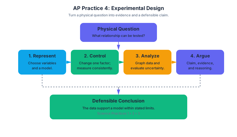
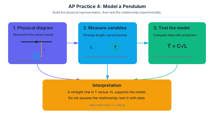
AP Practice 5
A strong physics response can begin with a picture or a sentence and end with an equation. The crucial skill is moving accurately between those forms: this practice focuses on qualitative-to-quantitative translation, especially turning a physical description and diagram into a symbolic model, then using that model…
AP Practice 5
A strong physics response can begin with a picture or a sentence and end with an equation. The crucial skill is moving accurately between those forms: this practice focuses on qualitative-to-quantitative translation, especially turning a physical description and diagram into a symbolic model, then using that model to compare outcomes.
Task focus: Translate a physical situation into representations, derive a symbolic relationship, and use that relationship to calculate or compare quantities.
This task combines Science Practice 1: Creating Representations and Science Practice 2: Mathematical Routines. It may also require 1.A. Create diagrams, tables, charts, or schematics to represent physical situations, 1.C. Create qualitative sketches of graphs that represent features of a model or the behavior of a physical system, 2.A. Derive a symbolic expression from known quantities by selecting and following a logical mathematical pathway, 2.B. Calculate or estimate an unknown quantity with units from known quantities, by selecting and following a logical computational pathway, and 2.C. Compare physical quantities between two or more scenarios or at different times and locations in a single scenario.
An original translation task: launching a cart
A laboratory cart of mass $m$ starts from rest at the top of a frictionless ramp. The cart descends through a vertical height $h$ and leaves the ramp with speed $v$. A second cart has mass $2m$ and descends through the same vertical height on the same frictionless ramp.
(a) Derive an expression for the speed $v$ of the first cart in terms of $g$ and $h$.
(b) Determine the speed of the second cart as it leaves the ramp.
(c) The ramp is changed so that the first cart descends through vertical height $4h$. Compare its new exit speed with the original speed.
Step 1: Build the physical representation
The important information is not the ramp’s length or angle. The cart’s vertical drop determines the change in gravitational potential energy. Because the ramp is frictionless, no mechanical energy is transformed into thermal energy.
A useful representation labels the initial and final states:
- Initial: $v_i = 0$, gravitational potential energy $U_i = mgh$
- Final: $v_f = v$, gravitational potential energy chosen as $U_f = 0$
- System: cart plus Earth
- External work that changes mechanical energy: none
This is 1.A. Create diagrams, tables, charts, or schematics to represent physical situations in action. The system boundary matters: including Earth allows gravitational potential energy to appear in the energy model.
Step 2: Derive before substituting
For the cart–Earth system, conservation of mechanical energy gives
$$ K_i + U_i = K_f + U_f. $$
Substitute the conditions at the two locations:
$$ 0 + mgh = \frac{1}{2}mv^2 + 0. $$
Cancel the mass $m$ and solve symbolically:
$$ gh = \frac{1}{2}v^2 $$
$$ v^2 = 2gh $$
$$ \boxed{v = \sqrt{2gh}}. $$
This earns the reasoning associated with 2.A. Derive a symbolic expression from known quantities by selecting and following a logical mathematical pathway. Notice why a symbolic derivation is more powerful than immediately inserting numbers: it exposes which variables matter and which cancel.
Step 3: Translate the comparison
For the second cart, the mass is $2m$, but the vertical drop remains $h$:
$$ 2mgh = \frac{1}{2}(2m)v_2^2. $$
The factor $2m$ appears on both sides and cancels:
$$ v_2 = \sqrt{2gh}. $$
Therefore,
$$ \boxed{v_2 = v}. $$
The heavier cart exits with the same speed, provided the ramp is frictionless and both carts start from rest at the same height. This is 2.C. Compare physical quantities between two or more scenarios or at different times and locations in a single scenario.
For a drop of $4h$,
$$ v_3 = \sqrt{2g(4h)} = \sqrt{8gh} = 2\sqrt{2gh}. $$
Since $v = \sqrt{2gh}$,
$$ \boxed{v_3 = 2v}. $$
The height is multiplied by $4$, but the speed is multiplied by only $2$ because speed depends on the square root of height. That proportional reasoning is often more important than the arithmetic.
Misconception check: “More mass means more speed”
Misconception: A heavier cart must reach the bottom faster because gravity pulls on it more strongly.
Correction: The heavier cart does experience a larger gravitational force, $F_g = mg$, but it also has proportionally greater inertia. In the energy equation, the same mass multiplies both the available gravitational energy and the kinetic-energy term, so mass cancels.
Examiner-rewarded reasoning would include the correct system, a valid conservation equation, a symbolic derivation, and a comparison justified by that expression. A bare answer such as “the speeds are equal” does not show the physical pathway.
Timing and error review
Spend about $2$ minutes identifying the system and representations, $4$ minutes deriving the expression, and $2$ minutes checking units and proportionality. Afterward, classify any error: representation error, principle-selection error, algebra error, comparison error, or unit error.
Quick retrieval check: If the ramp were rough and the cart lost mechanical energy to friction, would the exit speed be greater than, equal to, or less than $\sqrt{2gh}$? Explain using the system’s energy accounting.
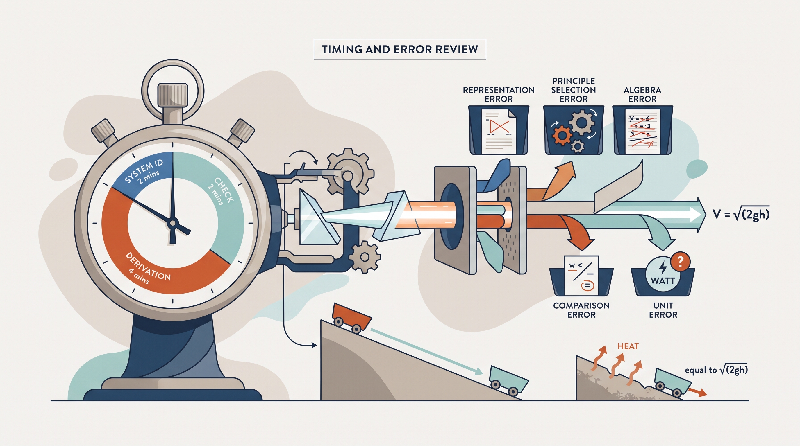
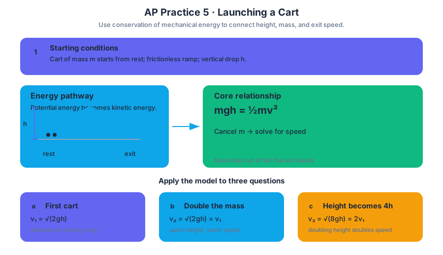
AP Practice 6
A successful physics investigation turns a physical question into measurable evidence: identify the variables, design a procedure, represent the data, and use a physical model to justify a conclusion.
AP Practice 6
A successful physics investigation turns a physical question into measurable evidence: identify the variables, design a procedure, represent the data, and use a physical model to justify a conclusion.
This practice targets an experimental design and analysis task, an exam task type that connects laboratory reasoning with the course’s three science practices: Science Practice 1: Creating Representations, Science Practice 2: Mathematical Routines, and Science Practice 3: Scientific Questioning and Argumentation.
Task: How does ramp angle affect the acceleration of a cart?
A student has a dynamics cart, a low-friction track, a motion sensor, a protractor, and a balance. The student wants to test the model that the cart’s acceleration down an inclined track depends on the component of gravitational force parallel to the track.
The student plans to vary the track angle $\theta$ and measure the cart’s acceleration $a$. For a simplified model with negligible friction,
$$ a = g\sin\theta $$
where $g$ is the local gravitational field strength.
Original practice prompt. Design an investigation that tests the model $a = g\sin\theta$. Your response should:
- identify the independent and dependent variables;
- describe how the data should be collected;
- specify a graph that could test the model;
- explain how the graph would support or challenge the model;
- identify one important source of uncertainty or systematic error;
- state how repeated trials improve the investigation.
Step 1: Build the experimental representation
The first move is not to write an equation. It is to represent the physical situation clearly. Draw the inclined track, label the angle $\theta$, show the cart’s direction of motion, and identify the measured quantities.
The independent variable is the quantity deliberately changed: the angle $\theta$. The dependent variable is the quantity that responds and is measured: the cart’s acceleration $a$.
Useful controlled variables include the same cart, the same track surface, the same release location, and the same motion sensor. Keeping these features fixed helps ensure that changes in measured acceleration are associated with $\theta$, rather than with a different cart or altered friction.
Step 2: Design a reproducible procedure
A strong procedure might be:
- Measure the track angle with a protractor and record $\theta$.
- Place the cart at the same release position for every trial.
- Release the cart without pushing it.
- Use the motion sensor to obtain a velocity-versus-time graph.
- Determine the slope of the best-fit line; this slope is the acceleration $a$.
- Repeat the measurement several times for the same angle.
- Repeat the entire process for several different values of $\theta$.
This procedure earns its strength from operational definitions. “Acceleration” does not mean merely that the cart is speeding up; here it is quantitatively defined as the slope of the velocity-versus-time graph:
$$ a = \frac{\Delta v}{\Delta t} $$
Science Practice 3: Scientific Questioning and Argumentation is visible in the testable question, the controlled procedure, and the planned evidence. A claim such as “steeper ramps produce greater acceleration” becomes scientific only when linked to measurements and a model.
Step 3: Choose the graph that tests the model
Because the model predicts $a = g\sin\theta$, the most direct graph is $a$ on the vertical axis versus $\sin\theta$ on the horizontal axis.
If the model is correct, the data should approximately form a straight line through the origin:
$$ a = g(\sin\theta) $$
The slope should be approximately $g$, with units of $\mathrm{m,s^{-2}}$.
This graph demonstrates Science Practice 1.B. Create quantitative graphs with appropriate scales and units, including plotting data. The horizontal axis must be labeled $\sin\theta$, which is dimensionless, and the vertical axis must be labeled $a$ in $\mathrm{m,s^{-2}}$. Plotting $a$ against $\theta$ directly may produce a curved relationship, so the transformed variable $\sin\theta$ is essential.
Step 4: Interpret evidence and uncertainty
Suppose the best-fit line has slope $8.7\ \mathrm{m,s^{-2}}$ and a small positive intercept. The slope is reasonably close to $g \approx 9.8\ \mathrm{m,s^{-2}}$, which supports the model, although friction may explain why the measured slope is smaller.
A positive intercept could indicate a systematic error, such as the motion sensor’s acceleration calibration or an incorrect estimate of the angle. A random release variation would instead cause trial-to-trial scatter without necessarily shifting every measurement in the same direction.
Repeating trials allows the student to estimate the spread in measured accelerations and identify anomalous results. Repetition does not automatically remove systematic error: measuring every angle incorrectly will produce consistently biased data.
What the examiner rewards
For this original, unofficial task, a high-scoring response would provide evidence aligned with the official practices and mathematical routines:
- 1.A. Create diagrams, tables, charts, or schematics to represent physical situations: a labeled ramp-and-cart diagram or organized data table.
- 1.B. Create quantitative graphs with appropriate scales and units, including plotting data: a graph of $a$ versus $\sin\theta$ with labels and units.
- 2.A. Derive a symbolic expression from known quantities by selecting and following a logical mathematical pathway: connect the predicted relation $a = g\sin\theta$ to the graph’s slope.
- 2.B. Calculate or estimate an unknown quantity with units from known quantities, by selecting and following a logical computational pathway: determine $g$ from the slope or calculate $a$ for a chosen angle.
- 3. Scientific Questioning and Argumentation: state a claim, cite the graph or measured values as evidence, and explain whether the evidence supports the model.
Timing and error review
Use approximately $12$–$15$ minutes for a first attempt: $2$ minutes to identify variables, $5$ minutes to design the procedure, $3$ minutes to select and explain the graph, and the remaining time to address uncertainty and repeated trials.
Afterward, classify each missed point as one of four errors: representation—the physical setup was unclear; mathematical—the model or slope was mishandled; experimental—a variable or uncertainty was overlooked; or argumentation—the claim was not connected to evidence. Then rewrite only the weakest response using a diagram, equation, or evidence statement.
Retrieval check
Why is $a$ plotted against $\sin\theta$ rather than directly against $\theta$? What physical meaning does the slope have if the model is correct?
Answer: The model predicts $a = g\sin\theta$, so $a$ versus $\sin\theta$ should be linear. The slope represents $g$, with units of $\mathrm{m,s^{-2}}$.
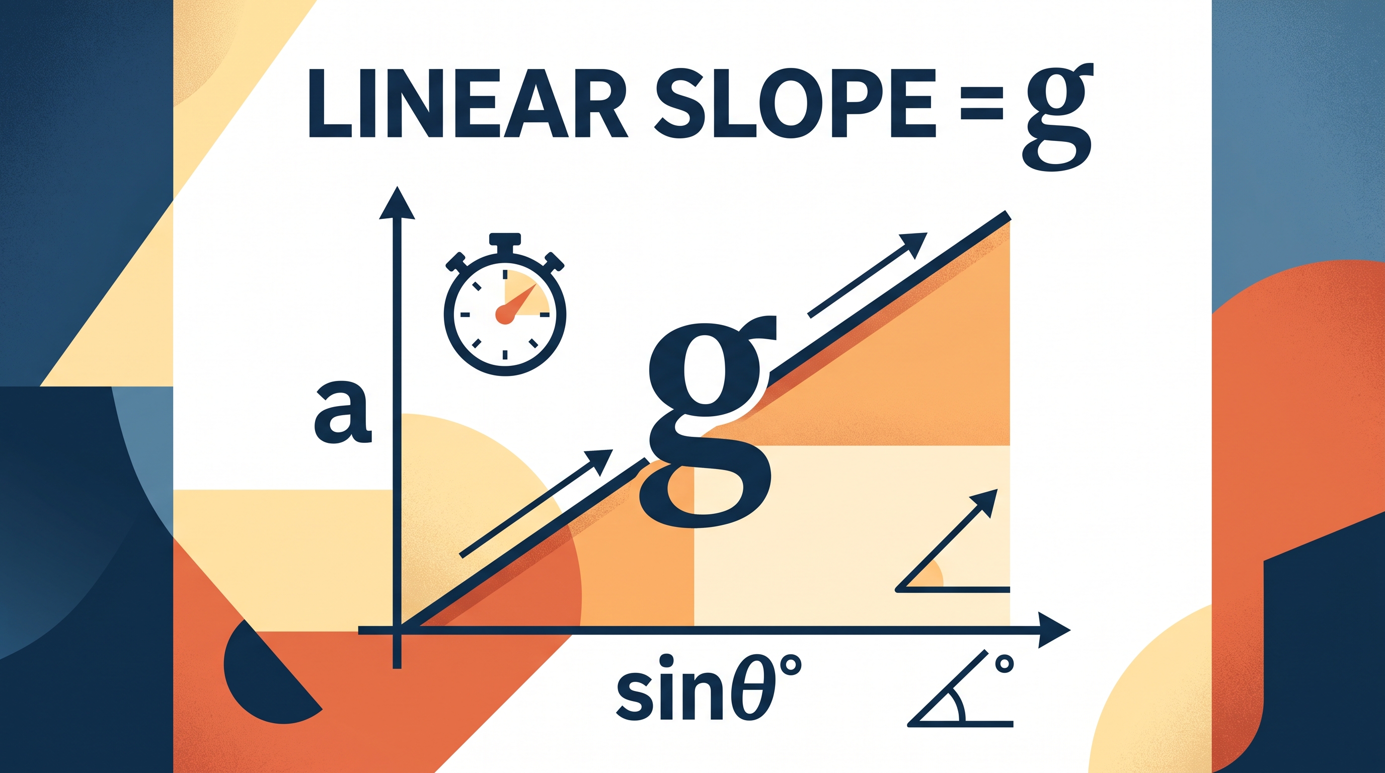
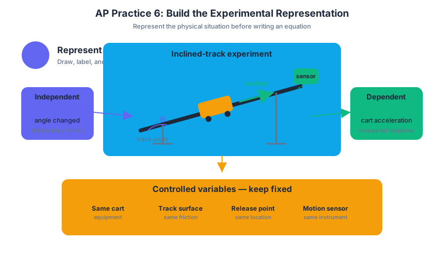
Source Materials
- Review the Exam Updates (.pdf)
- AP Physics 1: Algebra-Based Course and Exam Description
- AP Physics 1 Course Overview
- AP Physics 1 Course at a Glance
- AP Physics 1 Course at a Glance Poster
- Adopt AP Physics 1: Algebra-Based
- AP Physics 1: Algebra-Based
- AP Physics 1: Algebra-Based
- Figure — AP Physics 1: Algebra-Based Course and Exam Description (p. 1)
- Figure — AP Physics 1: Algebra-Based Course and Exam Description (p. 14)
- TOPICS
- Framework V.1 | 13 13
Study AP Physics 1 with AI — Free on Lykke
Sign up for free to generate personalized flashcards, quizzes, and study guides from this course. Chat with an AI tutor that knows the material.
Get Started FreeView this course wiki on Lykke · Browse all public course wikis