AP Microeconomics
Institution: MIT
111 study materials · 43 sections
AP Microeconomics students working the current College Board Course and Exam Description, including first-time students with no prior background, plus teachers reviewing the page for CED alignment.; Teach every official CED unit and every numbered topic at topic granularity.; Develop every AP skill / science-practice code explicitly and by name.; Replace description with teaching: worked contextual examples, named misconceptions, and in-flow retrieval checks.; Build an exam-practice unit covering every task type on the current exam.
Course Sections
Course Framework, Skills and Reasoning Processes
Key concepts: AP course framework · College-level microeconomics · Individual economic decision-makers · Big ideas and cross-cutting concepts · Conceptual understandings · Course skills and skill categories · Skill transfer and repetition · Unit sequencing and pacing · Instructional scaffolding · Student assessment and actionable feedback
AP Microeconomics studies how individual economic decision-makers—consumers, workers, and firms—make choices when resources are scarce. Its central move is to use economic principles and models to describe a situation, predict an outcome, and explain that outcome with words, graphs, charts, or data.
Course Framework, Skills and Reasoning Processes
AP Microeconomics studies how individual economic decision-makers—consumers, workers, and firms—make choices when resources are scarce. Its central move is to use economic principles and models to describe a situation, predict an outcome, and explain that outcome with words, graphs, charts, or data.
Course framework: The organized statement of the content, conceptual understandings, and skills students are expected to know and use.
The framework is designed for an introductory college-level course. It identifies required knowledge and reasoning without prescribing one fixed curriculum: teachers may sequence the six units differently, but students must encounter the required content and develop the associated skills.
The framework’s three layers
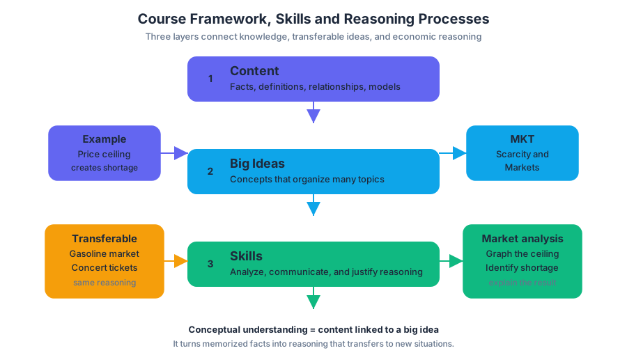
The framework connects three layers of understanding:
| Layer | What it contributes | Microeconomics example |
|---|---|---|
| Content | The facts, definitions, relationships, and models | A binding price ceiling creates a shortage |
| Big ideas | Cross-cutting concepts that organize many topics | MKT: Scarcity and Markets |
| Skills | The actions used to analyze and communicate economic reasoning | Graph the ceiling, identify the shortage, and explain the result |
A conceptual understanding is the durable relationship that links content to a big idea and makes the content usable in a new situation. It is more powerful than memorizing an isolated fact. For example, “a tax creates a wedge between the price buyers pay and the price sellers receive” is content; the conceptual understanding is that government intervention changes incentives and therefore alters market outcomes, surplus, and efficiency. That understanding can transfer from a market for gasoline to a market for concert tickets.
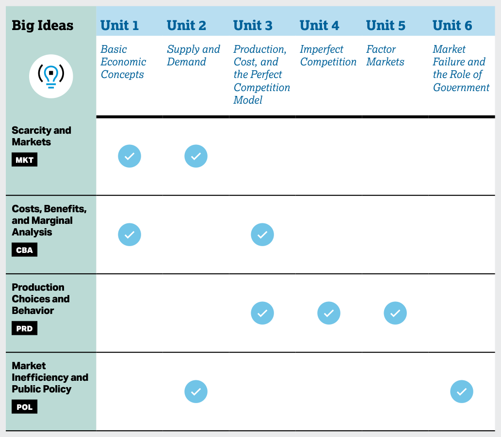
The four course-wide Big Ideas are:
- MKT: Scarcity and Markets — choices arise because resources are limited, and markets coordinate many individual decisions.
- CBA: Costs, Benefits, and Marginal Analysis — rational decision-makers compare additional benefits with additional costs.
- PRD: Production Choices and Behavior — firms choose inputs, output, and market strategies in pursuit of economic goals.
- POL: Market Inefficiency and Public Policy — markets can produce inefficient or inequitable outcomes, creating questions about intervention.
These ideas recur across units rather than belonging to only one topic. For instance, a pollution externality is POL, but analyzing it also uses CBA because the socially efficient quantity balances marginal social benefit and marginal social cost.
The four course skill categories
Skill Category 1: Principles and Models requires students to identify and explain economic concepts, principles, and models. A student might define opportunity cost, state the profit-maximization rule, or explain why a perfectly competitive firm is a price taker.
Skill Category 2: Interpretation requires students to explain an economic outcome in a specific context. The task is not merely to name “shortage,” but to connect a binding price ceiling to excess quantity demanded and explain what that means for buyers and sellers.
Skill Category 3: Manipulation requires students to determine how a change affects an economic situation. Examples include tracing a demand shift, calculating a new equilibrium, determining the effect of a wage change on labor demand, or identifying how a tariff changes domestic market outcomes.
Skill Category 4: Graphing and Visuals requires students to represent and analyze economic relationships with correctly labeled graphs, charts, and other visual tools. A complete graph communicates variables, curves, equilibrium points, shifts, and relevant areas such as consumer or producer surplus.
These skills work together. On a free-response question, a student may identify a negative externality using Principles and Models, explain the inefficient outcome through Interpretation, determine the effect of a corrective policy through Manipulation, and show the result on a graph through Graphing and Visuals. Multiple-choice questions can test any one skill or combine several; free-response questions especially reward visible reasoning, accurate calculations, labeled graphs, and contextual explanations.
Units, pacing, and instructional planning
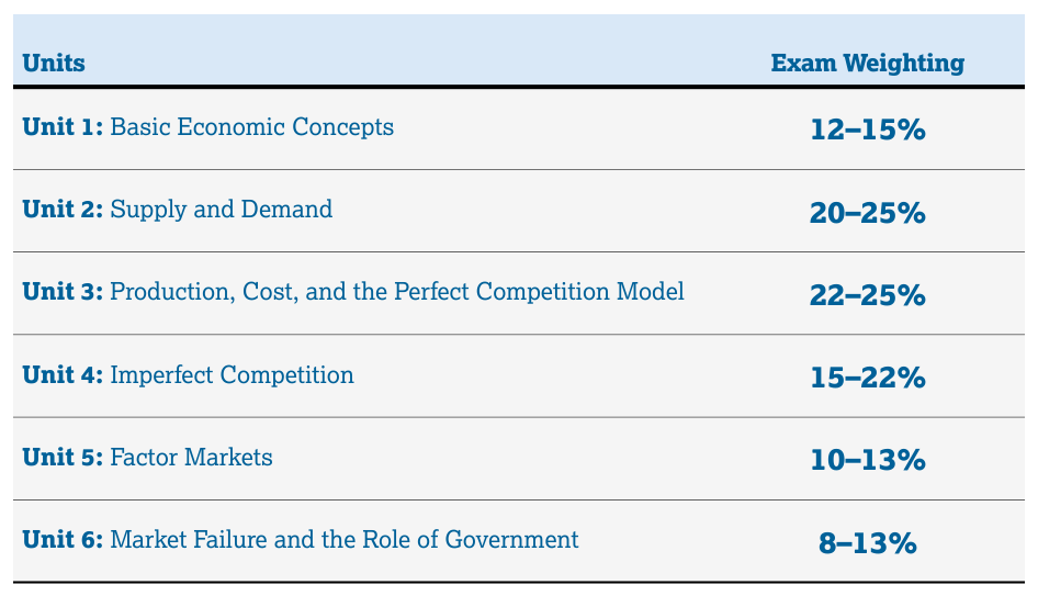
The six-unit sequence moves from individual choice and market foundations toward firms, factor markets, and public policy. The published multiple-choice weighting gives teachers a useful planning signal:
| Unit | Focus | Multiple-choice weighting | Approximate instructional guidance* |
|---|---|---|---|
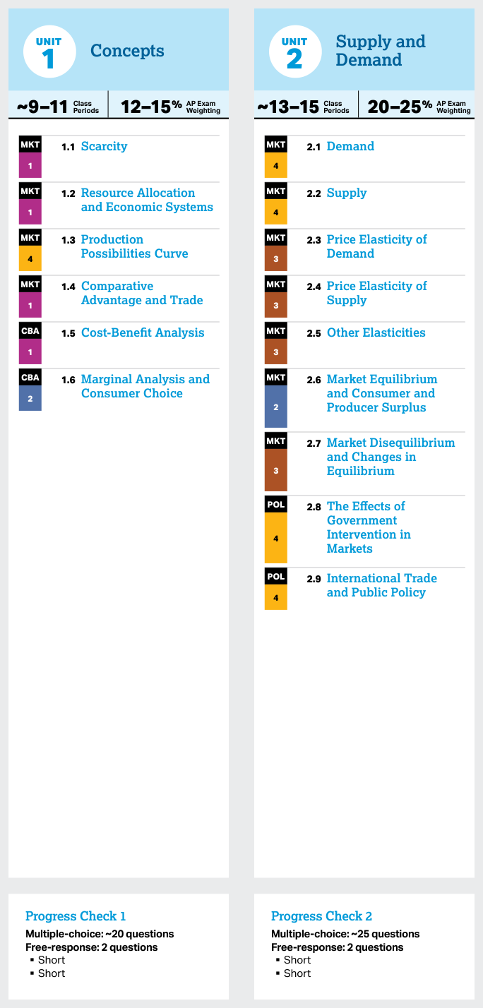
| 1 | Basic Economic Concepts | 12%–15% | 9–11 class periods |
| 2 | Supply and Demand | 20%–25% | 20–22 class periods |
| 3 | Production, Cost, and Perfect Competition | 17%–20% | 18–20 class periods |
| 4 | Imperfect Competition | 15%–18% | 15–17 class periods |
| 5 | Factor Markets | 10%–13% | 10–12 class periods |
| 6 | Market Failure and the Role of Government | 13%–16% | 13–15 class periods |
*These are planning estimates, not required outcomes.
Unit 2 commonly needs extra time because supply, demand, elasticity, equilibrium, intervention, and trade become the graphical and analytical vocabulary used later. Units 3 and 4 also deserve substantial time because students must connect production tables, cost curves, revenue, market structure, and firm behavior. A teacher may shorten a unit when diagnostic evidence shows mastery, or extend it when students need more graphing, calculation, or explanation practice.
A practical pacing cycle is introduce, scaffold, practice, transfer, and assess. Early practice can supply partially labeled graphs or structured calculation steps. Later practice should remove those supports and present unfamiliar contexts so students transfer the same reasoning to a new market. Reserve recurring time for retrieval, cumulative review, and feedback rather than placing all exam preparation at the end.
Planning, teaching, and assessment
The Unit at a Glance table helps teachers locate topics that build toward a common understanding, estimate pacing, and see how Big Ideas and skills spiral across the course. Unit overviews provide essential questions, conceptual understandings, and associated skills; topic pages specify the required content. Teachers should use those relationships to identify where scaffolding is needed—for example, reviewing marginal analysis before asking students to maximize profit.
Assessment should measure both what students know and what they can do with it. AP Classroom Progress Checks, original practice, graph analysis, numerical work, and written explanations can reveal whether an error is conceptual, graphical, computational, or interpretive. Useful feedback names the precise repair: “Your demand shift is correct, but you moved price along the old supply curve incorrectly,” rather than simply marking the response wrong.
The goal is economist-like reasoning: use a model, state the relevant assumption, trace the mechanism, represent the result accurately, and explain its meaning in context. Repeated practice across multiple-choice and free-response formats builds the flexibility needed to apply the same principles to unfamiliar economic situations.




1.1 Scarcity** `[MKT]`
Key concepts: Scarcity · Incentives and constraints · Mutually beneficial terms of trade · Utility · Profit-maximizing strategy · Strategic decision-making
A community can want unlimited clean water, leisure, food, shelter, and entertainment, but it cannot command unlimited time, money, labor, or materials. Scarcity exists because human wants exceed the resources available to satisfy them.
1.1 Scarcity** [MKT]
A community can want unlimited clean water, leisure, food, shelter, and entertainment, but it cannot command unlimited time, money, labor, or materials. Scarcity exists because human wants exceed the resources available to satisfy them. Every choice therefore has a cost: selecting one use of a resource means giving up another.
Investigative question: When resources are limited, how do incentives, constraints, and trade help people and firms make choices?
Scarcity forces choices
A student with two free hours might work at a café, study for an exam, exercise, or meet friends. The student cannot fully choose all four uses of the same two hours. A constraint is a limitation on available choices, such as time, income, technology, information, or productive capacity. An incentive is something that encourages or discourages an action, such as a wage, a price, a reward, a penalty, or an expected profit.
The important point in MKT-3: Individuals and firms respond to incentives and face constraints is that choices arise from the interaction of both forces. A higher wage may encourage a person to work more, but a demanding school schedule may limit how many hours are actually available. A firm may want to produce more, but limited machinery, workers, or materials constrain its output.
A useful decision chain is:
$$ \text{Scarcity} \longrightarrow \text{Constraints} \longrightarrow \text{Trade-offs} \longrightarrow \text{Choices shaped by incentives} $$
Misconception check — “Scarcity means a good is rare.” Scarcity does not require physical rarity. Even abundant goods can be scarce if obtaining, storing, or distributing them requires limited resources. Air is generally not scarce for breathing, but clean air in a polluted city may be scarce because its quality is limited relative to demand.
Mutually beneficial terms of trade
Scarcity does not mean every person must produce everything independently. Trade allows people or firms to exchange goods, services, or resources. Mutually beneficial terms of trade are exchange conditions under which both parties become better off than they would have been without the exchange.
Suppose Maya can bake bread efficiently but dislikes repairing bicycles, while Luis repairs bicycles efficiently but has little time for baking. Maya gives Luis bread, and Luis repairs Maya’s bicycle. If each person values what they receive more than what they give up, both gain—even though no new physical resources appeared. Trade improves the allocation of existing scarce resources by allowing specialization and exchange.
The exchange must be voluntary and acceptable to both sides. If Maya would accept at least one bicycle repair for two loaves of bread, while Luis would provide that repair for no more than three loaves, any agreed exchange between those amounts can benefit both participants.
Utility: measuring benefit from consumption
Utility is the benefit or satisfaction a consumer receives from consuming a good or service. Utility is not necessarily measured in dollars; economists use it as a way to represent how strongly a consumer values different options.
For example, a hungry customer may receive high utility from the first sandwich but less additional utility from a second sandwich. The customer still faces an income constraint, so the choice depends on both the satisfaction available from each purchase and the prices of the goods. Utility explains the benefit side of a consumer decision; scarcity explains why the consumer cannot simply purchase every desirable option.
Worked example: Field Cruiser
Field Cruiser is deciding how to improve its vehicle. Its scarce development budget can be directed toward greater Power or another feature. The firm compares the expected additional revenue or cost savings from each strategy with the resources required to implement it.
When the available incentives, expected benefits, and production constraints are evaluated together, Field Cruiser’s most profitable strategy is to improve Power. The conclusion is not that Power is universally the best feature. It is the best strategy under Field Cruiser’s particular constraints and expected returns.
This is a simple example of strategic decision-making: choosing an action after considering how scarce resources, expected payoffs, and constraints interact. A profit-maximizing firm selects the strategy expected to produce the greatest economic profit, not necessarily the strategy with the greatest sales, popularity, or physical output.
AP skill connection
This topic most directly uses Skill Category 1: Principles and Models, especially 1.A Define economic principles and models and 1.B Explain economic principles and models; Skill Category 2: Interpretation, including 2.A Identify economic concepts, principles, and models and 2.B Explain economic outcomes; and Skill Category 3: Manipulation, including 3.A Determine outcomes of specific economic situations. On an exam, these skills may appear through a short scenario, a comparison of incentives and constraints, or a request to identify the firm’s most profitable strategy.
Retrieval check: A worker receives a higher wage but cannot work additional hours because of a fixed school schedule. Which force limits the worker’s response: an incentive or a constraint? Why can a voluntary exchange make both parties better off?
![1.1 Scarcity** `[MKT]` - AP Microeconomics - image 1](https://getlykke-assets.s3.amazonaws.com/wiki-images/1cc499d1-b83b-410f-98ef-13739a940956_1_1_Scarcity_____MKT__.jpeg)
![1.1 Scarcity** `[MKT]` - AP Microeconomics - image 2](https://getlykke-assets.s3.amazonaws.com/wiki-figures/aeb7daea6ee11b01_ap25_frq_microeconomics_set_2_pdf_p4_0.png)
![1.1 Scarcity** `[MKT]` - AP Microeconomics - diagram 1](https://www.getlykke.com/explore/public/ap-microeconomics/media/topic-1-1/svg/1)
1.2 Resource Allocation and Economic Systems** `[MKT]`
Key concepts: Scarcity · Resource allocation · Economic systems · Factors of production · Non-rival resources · Incentives and constraints · Market prices · Market demand curves
A society must answer three linked questions whenever it directs inputs toward production: what goods and services to produce, how to produce them, and who consumes them.
1.2 Resource Allocation and Economic Systems** [MKT]
A society must answer three linked questions whenever it directs inputs toward production: what goods and services to produce, how to produce them, and who consumes them. The answers determine whether a city uses a valuable waterfront for apartments, a public park, a factory, or some combination—and whether those decisions are made through prices, government direction, custom, or a mixture of systems.
The allocation problem
Resource allocation is the process of deciding how available resources are assigned among competing uses. The relevant resources include the factors of production: land (natural resources and physical space), labor (human effort), and capital (produced tools, equipment, and structures used to make other goods and services).
| Allocation question | Example for a city |
|---|---|
| What to produce? | More housing, restaurants, schools, or parks? |
| How to produce it? | With labor-intensive construction or automated equipment? |
| Who consumes it? | Whoever can pay, whoever is selected by public rules, or everyone through shared access? |
Allocation depends especially on whether an input is rival: one person’s use prevents, or reduces, another person’s use of that same unit. A construction site, delivery truck, nurse’s working time, and parcel of land are rival inputs. Assigning them to one project means they cannot simultaneously serve competing projects, so decision-makers must compare uses and respond to constraints.
Some resources are non-rival, meaning one person’s use does not substantially reduce another person’s ability to use them. Established knowledge—such as a production technique or a mathematical formula—can often be used by many firms at once. A firm may still need scarce labor, computers, or legal access to apply that knowledge, but the knowledge itself does not become unavailable merely because another firm uses it.
Economic systems shape allocation
An economic system is the set of rules and institutions a society uses to organize production and consumption. Because systems assign decision-making authority differently, they produce different answers to the three allocation questions.
- A market economy relies primarily on decentralized decisions by households and firms. Prices communicate information about relative scarcity and guide resources toward uses for which buyers are willing to pay.
- A command economy relies primarily on government decisions. Public authorities determine production targets, methods, and distribution rules.
- A mixed economy combines markets with government action. Prices allocate many resources, while laws, taxes, subsidies, public production, or regulation alter particular outcomes.
No system eliminates constraints. A market economy may allocate housing toward high-income buyers rather than toward families with the greatest need. A command system may direct resources toward a public priority but lack accurate information about consumers’ changing preferences. The important economic question is not whether choices occur—they must—but who makes them and what incentives guide them.
Incentives and constraints
An incentive is a reward or penalty that changes the benefit or cost of an action. A higher wage can encourage workers to enter an occupation; a profit opportunity can encourage firms to produce a good; a tax can discourage an activity; and a subsidy can encourage it. A constraint is a limit on the actions available, such as income, time, technology, laws, or the quantity of land and labor.
Worked example — a neighborhood bakery: A bakery has one oven, a fixed number of workers, and limited flour. It must decide whether to produce bread, pastries, or both (what); whether to use more workers or specialized equipment (how); and which customers receive the output if demand exceeds production capacity (who). If the price of pastries rises, the potential profit creates an incentive to shift resources toward pastries—but the oven and staff remain constraints.
The bakery’s decision is also connected to consumers. The market demand curve is derived by adding the quantities demanded by all individual buyers at each possible price. If one buyer demands $2$ loaves at a price of $4$, a second demands $3$, and a third demands $1$, market quantity demanded at $4 is:
$$ Q_D^{market}=2+3+1=6\text{ loaves} $$
As prices change, the summed quantities show how the market communicates collective willingness to purchase. Sellers then use the resulting price signals, together with production costs and available inputs, to help allocate scarce resources.
Misconception check
Misconception: “A market economy means the government has no role.” A market economy uses prices and private decisions as its primary allocation mechanism, but a mixed economy may also use taxes, regulations, public goods, and other policies. Misconception: “Knowledge is always scarce because resources are scarce.” Knowledge can be non-rival even when the labor, equipment, and time required to create or apply it are rival and scarce.
Retrieval check
A town can use a vacant lot for a clinic or a shopping center. Identify the allocation question involved, name one rival factor of production that constrains the choice, and explain how a higher expected profit from shopping-center construction could change the town’s allocation decision. Then state why the town’s market demand curve cannot be found by looking at only one buyer’s demand.
![1.2 Resource Allocation and Economic Systems** `[MKT]` - AP Microeconomics - image 1](https://getlykke-assets.s3.amazonaws.com/wiki-images/9fcc5a7c-4f00-4894-8244-fa0902050ae1_1_2_Resource_Allocation_and_Economic_Systems_____MKT__.jpeg)
![1.2 Resource Allocation and Economic Systems** `[MKT]` - AP Microeconomics - diagram 1](https://www.getlykke.com/explore/public/ap-microeconomics/media/topic-1-2/svg/1)
1.3 Production Possibilities Curve** `[MKT]`
Key concepts: Production Possibilities Curve (PPC) · Scarcity · Trade-offs · Resource allocation · Opportunity cost · Efficiency · Underutilized resources · Economic growth and contraction · PPC shape and opportunity costs · Factors of production and productivity
A society cannot produce unlimited amounts of everything because its resources are scarce. The production possibilities curve (PPC) is a model that makes the resulting trade-offs visible: it shows the maximum combinations of two goods or services that can be produced with available resources, technology, and…
1.3 Production Possibilities Curve** [MKT]
A society cannot produce unlimited amounts of everything because its resources are scarce. The production possibilities curve (PPC) is a model that makes the resulting trade-offs visible: it shows the maximum combinations of two goods or services that can be produced with available resources, technology, and productive knowledge.
MKT-1.C.1: The PPC is a model used to show the trade-offs associated with allocating resources.
Reading the PPC
Imagine an economy producing only solar panels and electric bicycles. Every point on the curve represents a possible allocation of labor, capital, land, and entrepreneurship between those two products. Moving along the curve toward more solar panels requires producing fewer electric bicycles.
The three regions of the graph answer two questions: Is the combination feasible? and Is it using resources efficiently?
| Location | Feasible with current resources? | Economic meaning |
|---|---|---|
| On the PPC | Yes | Productively efficient: available resources are fully and appropriately used |
| Inside the PPC | Yes | Inefficient: resources are underutilized or misallocated |
| Outside the PPC | No | Currently unattainable without more resources or better productivity |
A point inside the curve might represent unemployed workers, idle factories, or production organized poorly. It is feasible, but the economy could produce more of at least one good without sacrificing the other. A point outside the curve is desirable perhaps, but unattainable under current conditions.
MKT-1.C.2: The PPC can be used to illustrate scarcity, opportunity cost, efficiency, underutilized resources, and economic growth or contraction.
Trade-offs and opportunity cost
A trade-off is what must be given up to obtain something else. Opportunity cost is the specific next-best alternative forgone. On a PPC, the opportunity cost of producing additional units of one good is measured by the amount of the other good sacrificed.
Suppose the economy can produce the following combinations:
| Combination | Solar panels | Electric bicycles |
|---|---|---|
| A | $0$ | $40$ |
| B | $1$ | $36$ |
| C | $2$ | $30$ |
| D | $3$ | $20$ |
| E | $4$ | $0$ |
Moving from B to C increases solar-panel production by $1$ but reduces electric-bicycle production by $6$. Therefore, the opportunity cost of that additional solar panel is $6$ electric bicycles. Moving from C to D has an opportunity cost of $10$ electric bicycles:
$$ \text{Opportunity cost of one additional solar panel}
\frac{\text{electric bicycles forgone}}{\text{solar panels gained}}
\frac{10}{1}
10\text{ electric bicycles} $$
The economy faces a changing trade-off because resources are not equally productive in both uses. Workers and machines especially suited to bicycle production may be shifted first; producing still more solar panels eventually requires reallocating resources that are better suited to bicycles.
Why the curve has different shapes
The shape of the PPC depends on how opportunity cost changes as production shifts between goods.
- A constant opportunity-cost PPC is a straight line. Resources are equally adaptable between the two goods, so each additional unit costs the same amount of the other good.
- An increasing opportunity-cost PPC is bowed outward, or concave. Resources become progressively less suited to the good whose production is expanding.
- A decreasing opportunity-cost PPC is bowed inward, or convex. Specialization makes additional production increasingly efficient, so each extra unit costs less of the other good.
MKT-1.C.3: The shape of the PPC depends on whether opportunity costs are constant, increasing, or decreasing.
Movement along the curve versus a shift
A movement along a PPC changes the economy’s product mix while resources and technology remain fixed. It represents a trade-off, not economic growth: producing more of one good requires producing less of the other.
A shift of the entire PPC changes what the economy can produce. An outward shift represents economic growth; an inward shift represents economic contraction.
The PPC shifts outward when the economy gains productive resources or improves productivity—for example, through a larger labor force, more capital, additional usable land, better worker knowledge, or improved technology. A natural disaster that destroys factories, a loss of workers, or a decline in productivity can shift the PPC inward.
MKT-1.C.4: The PPC can shift due to changes in factors of production as well as changes in productivity/technology.
MKT-1.C.5: Economic growth results in an outward shift of the PPC.
When drawing a shift, use arrows to show the direction clearly. A change affecting both goods generally shifts the whole curve outward or inward. A productivity improvement affecting only solar panels rotates the PPC outward mainly along the solar-panel axis rather than moving every point equally.
Resource allocation and AP reasoning
The PPC connects scarcity to resource allocation: society must decide what goods and services to produce, how to produce them, and for whom they are produced. The chosen point reflects those decisions, while the curve shows the limits imposed by available resources and technology.
This topic uses all four AP skill categories:
- Skill Category 1: Principles and Models — define the PPC, scarcity, efficiency, and opportunity cost.
- Skill Category 2: Interpretation — explain what a point, movement, or shift means in a specific economic situation.
- Skill Category 3: Manipulation — calculate opportunity cost from a table and determine how a resource or productivity change affects feasible output.
- Skill Category 4: Graphing and Visuals — draw and label axes, plot feasible combinations, identify efficiency, and use arrows to show outward or inward shifts.
Misconception check
Misconception: “Every point inside the PPC is impossible.”
Correction: points inside the curve are feasible but inefficient. The impossible points are outside the current PPC. Also, a point on the curve is productively efficient, but that does not automatically mean it is the society’s preferred or socially fairest allocation.
Retrieval check
An economy moves from a point on its PPC to another point on the same PPC, producing more medical equipment and fewer restaurants. Is this an economic contraction? No. It is a movement along the curve, showing a trade-off and an opportunity cost. A contraction would shift the entire PPC inward.
![1.3 Production Possibilities Curve** `[MKT]` - AP Microeconomics - image 1](https://getlykke-assets.s3.amazonaws.com/wiki-images/f245c249-8db0-4a82-8b19-62d8469dfaee_1_3_Production_Possibilities_Curve_____MKT__.jpeg)
![1.3 Production Possibilities Curve** `[MKT]` - AP Microeconomics - diagram 1](https://www.getlykke.com/explore/public/ap-microeconomics/media/topic-1-3/svg/1)
![1.3 Production Possibilities Curve** `[MKT]` - AP Microeconomics - diagram 2](https://www.getlykke.com/explore/public/ap-microeconomics/media/topic-1-3/svg/2)
1.4 Comparative Advantage and Trade** `[MKT]`
Key concepts: Absolute advantage · Comparative advantage · Opportunity cost · Specialization in production · Production possibilities curve (PPC) · Gains from trade · Terms of trade · Scarcity · Consumption possibilities beyond the PPC · Mutually beneficial trade
A producer can benefit from trade even when another producer is better at making everything. The key question is not “Who can produce more?” but “Who gives up less to produce this good?”
1.4 Comparative Advantage and Trade** [MKT]
A producer can benefit from trade even when another producer is better at making everything. The key question is not “Who can produce more?” but “Who gives up less to produce this good?”
Scarcity creates the reason to specialize
Resources are scarce: time, labor, land, tools, and materials have competing uses. When a producer uses those resources to make one good, the producer gives up some amount of another good. That forgone alternative is the opportunity cost of the choice.
Specialization directs scarce resources toward the use with the lowest opportunity cost. Trade then allows producers to exchange part of their specialized output for other goods, mitigating the consequences of scarcity.
Absolute advantage versus comparative advantage
Absolute advantage means producing a greater quantity of a good or service than another producer with the same quantity of resources. It is a comparison of productivity.
MKT-2.A.1: Absolute advantage describes a situation in which an individual, business, or country can produce more of a good or service than any other producer with the same quantity of resources.
Comparative advantage means producing a good or service at a lower opportunity cost than another producer. It is a comparison of what must be sacrificed.
MKT-2.A.2: Comparative advantage describes a situation in which an individual, business, or country can produce a good or service at a lower opportunity cost than another producer.
A producer may have an absolute advantage in both goods, but cannot have a comparative advantage in both goods. If one producer has the lower opportunity cost of producing one good, the other producer must have the lower opportunity cost of producing the other good.
Worked example: finding comparative advantage
Suppose Blair and Casey each have the same resources. In one production period, Blair can produce either $16$ baskets of fruit or $6$ shirts. Casey can produce either $12$ baskets of fruit or $4$ shirts.
Blair has the absolute advantage in both goods because Blair can produce more fruit and more shirts. But opportunity costs determine comparative advantage:
$$ \text{Blair's opportunity cost of 1 shirt}
\frac{16\text{ baskets of fruit}}{6\text{ shirts}}
\frac{8}{3}\text{ baskets of fruit} $$
$$ \text{Casey's opportunity cost of 1 shirt}
\frac{12\text{ baskets of fruit}}{4\text{ shirts}}
3\text{ baskets of fruit} $$
Because Blair gives up fewer baskets of fruit per shirt, Blair has the comparative advantage in shirts. Casey therefore has the comparative advantage in fruit: Casey gives up fewer shirts per basket of fruit.
To analyze a trade problem, calculate each producer’s opportunity costs, identify comparative advantage, and test whether the proposed terms of trade fall between those costs.
Specialization and gains from trade
Specialization in production occurs when each producer concentrates resources on the good for which that producer has comparative advantage. Blair specializes in shirts, while Casey specializes in fruit. Their combined production can exceed the combined production possible when each produces both goods independently.
Terms of trade are the rate at which one good exchanges for another. For trade to benefit both parties, the exchange rate must lie between their opportunity costs.
For one shirt, Blair requires at least $\frac{8}{3}$ baskets of fruit to avoid losing from trade, while Casey will pay up to $3$ baskets of fruit because producing one shirt costs Casey $3$ baskets. Therefore, mutually beneficial terms of trade for one shirt fall in the interval
$$ \frac{8}{3} < \text{terms of trade} < 3. $$
At a rate of $1$ shirt for $\frac{17}{6}$ baskets of fruit, Blair receives more fruit than Blair’s internal opportunity cost, and Casey pays less fruit than Casey’s internal opportunity cost. Both producers gain.
Why consumption can move beyond the PPC
A production possibilities curve shows what a producer can produce using available resources and technology. Trade does not necessarily move the producer’s own PPC; instead, it allows the producer to consume a combination that would have been unattainable through isolated production.
For example, if Blair specializes in shirts, produces $6$ shirts, and trades for $\frac{16}{3}$ baskets of fruit, Blair may consume a bundle containing $2$ shirts and $\frac{16}{3}$ baskets of fruit after trading away $4$ shirts. Measured against Blair’s fruit-only maximum of $16$ baskets and shirt maximum of $6$ shirts, the bundle’s normalized resource use is
$$ \frac{16/3}{16}+\frac{2}{6}
\frac{1}{3}+\frac{1}{3}
\frac{2}{3}, $$
which is feasible. If the intended bundle instead uses Blair’s relevant trade conversion of $\frac{16}{3}$ fruit units against a six-unit fruit scale, its normalized calculation is
$$ \frac{16/3}{6}+\frac{2}{6}
\frac{8}{9}+\frac{1}{3}
\frac{11}{9}>1. $$
That second representation places Blair’s consumption bundle beyond the original PPC: Blair could not reach it without trade. The economic conclusion is the important one—specialization based on comparative advantage and mutually beneficial exchange expands consumption possibilities.
MKT-2.B.1: Production specialization according to comparative advantage, not absolute advantage, results in exchange opportunities that lead to consumption possibilities beyond the PPC.
MKT-2.B.2: Comparative advantage and opportunity costs determine the terms of trade for exchange under which mutually beneficial trade can occur.
Misconception check
Misconception: “The producer with absolute advantage should produce both goods.” Absolute advantage identifies who can produce more, but comparative advantage identifies who sacrifices less. Producing according to absolute advantage alone can waste the gains created by different opportunity costs.
Retrieval check: If one country has a lower opportunity cost of producing wheat and another has a lower opportunity cost of producing machines, which country should specialize in wheat? What must be true of the terms of trade for both countries to gain?
![1.4 Comparative Advantage and Trade** `[MKT]` - AP Microeconomics - image 1](https://getlykke-assets.s3.amazonaws.com/wiki-images/2627a62d-538b-4d6c-a0ef-0d290b8be2f3_1_4_Comparative_Advantage_and_Trade_____MKT__.jpeg)
![1.4 Comparative Advantage and Trade** `[MKT]` - AP Microeconomics - image 2](https://getlykke-assets.s3.amazonaws.com/wiki-figures/56d8a6c1bbdfad15_ap23_cr_report_micro_set_1_pdf_p10_0.png)
![1.4 Comparative Advantage and Trade** `[MKT]` - AP Microeconomics - image 3](https://getlykke-assets.s3.amazonaws.com/wiki-figures/875143204c5796cb_ap23_frq_microeconomics_set_1_pdf_p4_0.png)
![1.4 Comparative Advantage and Trade** `[MKT]` - AP Microeconomics - diagram 1](https://www.getlykke.com/explore/public/ap-microeconomics/media/topic-1-4/svg/1)
1.5 Cost-Benefit Analysis** `[CBA]`
Key concepts: Cost-benefit analysis · Total benefits and total costs · Total net benefits · Marginal benefit and marginal cost · Rational economic decision-making · Profit maximization · Allocative efficiency · Market equilibrium · Deadweight loss · Per-unit subsidies and market inefficiency
A rational decision is not necessarily the decision with the greatest total benefit; it is the decision with the greatest total net benefit after every economic cost is counted.
1.5 Cost-Benefit Analysis** [CBA]
A rational decision is not necessarily the decision with the greatest total benefit; it is the decision with the greatest total net benefit after every economic cost is counted. That means including both the money paid and the opportunity cost of what must be given up.
From benefits and costs to the optimal choice
Cost-benefit analysis compares the total benefits of an action with its total economic costs. For a consumer, total benefit is commonly measured as utility; for a firm, it is commonly measured as total revenue. Economic cost includes explicit costs, such as wages or rent actually paid, and implicit costs, such as the income the owner sacrifices by using personal time or money in the business.
CBA-1.A.1: Total net benefits equal total benefits minus total economic costs, including both explicit and implicit costs.
The central calculation is:
$$ \text{Total Net Benefits}=\text{Total Benefits}-\text{Total Economic Costs} $$
Suppose a student is deciding whether to spend Saturday operating a snack stand. The stand earns $180$ in revenue. The student pays $70$ for ingredients and permits, but gives up $80$ that could have been earned at a tutoring job. Total economic cost is therefore $150$, not merely the $70$ paid out of pocket:
$$ \text{Total Economic Costs}=$70+$80=$150 $$
$$ \text{Total Net Benefits}=$180-$150=$30 $$
If the student instead attends a free concert, the decision may not be naturally divisible into one-unit increments. In that case, comparing total benefits and total costs is more useful than comparing marginal values. Under CBA-1.B.1, total net benefits are maximized at the optimal choice.
Marginal analysis: choosing the next unit
Some decisions can be separated into increments: one more hour worked, one more backpack produced, or one more unit sold. The marginal benefit is the additional benefit from one more unit; the marginal cost is the additional economic cost of that unit.
CBA-1.B.2: Rational economic agents compare marginal benefit and marginal cost when deciding whether and how much of an activity to pursue.
The decision rule is:
$$ \text{Pursue another unit if } MB \geq MC $$
Continue expanding an activity while marginal benefit exceeds marginal cost. Stop at the quantity where the next unit would add no more benefit than cost. When marginal benefit is decreasing and marginal cost is increasing, total net benefits are maximized generally where:
$$ MB=MC $$
Misconception check — “The best choice has the highest total benefit.” Not necessarily. A larger activity can generate more total benefit but also much larger total cost. The correct comparison is total benefit versus total economic cost, or—when the decision is divisible—marginal benefit versus marginal cost.
Firms: profit maximization
For a firm, the relevant benefit from selling one additional unit is marginal revenue—the change in total revenue from that unit. The firm maximizes economic profit by producing the quantity where marginal revenue equals marginal cost:
$$ MR=MC $$
In perfect competition, the firm is a price taker, so the price received for every additional unit is constant. Therefore:
$$ MR=P $$
For a firm with market power, marginal revenue is generally below the demand curve because selling additional output requires lowering the price. The firm first finds its output where $MR=MC$, then uses the demand curve to determine the price consumers will pay. This distinction matters: choosing the highest possible price does not generally maximize profit.
Cost calculations that reveal the decision
Two calculations frequently appear in cost-benefit problems:
$$ AFC=\frac{\text{Total Fixed Cost}}{\text{Quantity of Output}} $$
If total fixed cost is $$90$ and output is $30$ units:
$$ AFC=\frac{$90}{30}=$3 $$
Marginal cost measures the change in variable cost caused by a change in output:
$$ MC=\frac{\Delta TVC}{\Delta Q} $$
If total variable cost rises by $$6$ when output increases by one unit, marginal cost is $$6$. Fixed cost does not change when output changes in the short run, so it does not determine marginal cost.
Market efficiency, deadweight loss, and corrective policy
In a market graph, the demand curve can represent marginal benefit and the supply curve can represent marginal cost. The competitive equilibrium is allocatively efficient when the equilibrium quantity is where marginal benefit equals marginal cost.
If equilibrium output is $20$ backpacks but the allocatively efficient output is only $16$, the market is overproducing. The units between $16$ and $20$ cost more to produce than they are worth to buyers. The lost total surplus is deadweight loss, shown as the area between the marginal-benefit and marginal-cost curves over that excess-output range.
Misconception check — “A subsidy always fixes deadweight loss.” The correct policy depends on the direction of the inefficiency. With equilibrium quantity $20$ and efficient quantity $16$, a per-unit tax, not a subsidy, must reduce the private incentive to produce. If the marginal external cost is $$10$ per backpack at the efficient quantity, a $$10$ per-unit tax shifts private marginal cost upward by that wedge and can align private incentives with social cost.
Conversely, if equilibrium output is below the efficient quantity—for example, $16$ backpacks instead of $20$ because production creates a $$10$ marginal external benefit—a $$10$ per-unit subsidy shifts the private marginal-benefit incentive upward. It encourages the additional production whose social benefit exceeds its private benefit, eliminating the deadweight loss when the wedge is correctly measured.
Retrieval check: A firm’s total revenue is $$500$, explicit costs are $$300$, and implicit costs are $$120$. Its economic profit is $$80$. If the next unit adds $$14$ of revenue and $$11$ of cost, should the firm produce it? Yes: the additional unit raises total net benefits by $$3$, because $MB$ or $MR$ exceeds $MC$.
![1.5 Cost-Benefit Analysis** `[CBA]` - AP Microeconomics - image 1](https://getlykke-assets.s3.amazonaws.com/wiki-images/f00bce4e-34c9-4546-a1c1-4b46ee582c02_1_5_Cost-Benefit_Analysis_____CBA__.jpeg)
![1.5 Cost-Benefit Analysis** `[CBA]` - AP Microeconomics - image 2](https://getlykke-assets.s3.amazonaws.com/wiki-figures/e613842715b1726c_ap23_apc_microeconomics_q1_set_1_pdf_p4_0.png)
![1.5 Cost-Benefit Analysis** `[CBA]` - AP Microeconomics - image 3](https://getlykke-assets.s3.amazonaws.com/wiki-figures/1370dcee5028acbd_ap23_apc_microeconomics_q1_set_2_pdf_p3_1.png)
![1.5 Cost-Benefit Analysis** `[CBA]` - AP Microeconomics - image 4](https://getlykke-assets.s3.amazonaws.com/wiki-figures/8feb06fd59b827bf_ap23_apc_microeconomics_q1_set_2_pdf_p4_1.png)
![1.5 Cost-Benefit Analysis** `[CBA]` - AP Microeconomics - image 5](https://getlykke-assets.s3.amazonaws.com/wiki-figures/e613842715b1726c_ap23_sg_microeconomics_set_1_pdf_p4_0.png)
![1.5 Cost-Benefit Analysis** `[CBA]` - AP Microeconomics - image 6](https://getlykke-assets.s3.amazonaws.com/wiki-figures/1370dcee5028acbd_ap23_sg_microeconomics_set_2_pdf_p3_1.png)
![1.5 Cost-Benefit Analysis** `[CBA]` - AP Microeconomics - image 7](https://getlykke-assets.s3.amazonaws.com/wiki-figures/8feb06fd59b827bf_ap23_sg_microeconomics_set_2_pdf_p4_1.png)
![1.5 Cost-Benefit Analysis** `[CBA]` - AP Microeconomics - diagram 1](https://www.getlykke.com/explore/public/ap-microeconomics/media/topic-1-5/svg/1)
1.6 Marginal Analysis and Consumer Choice** `[CBA]`
Key concepts: Consumer constraints and choice · Marginal analysis · Marginal benefit · Marginal cost · Marginal utility · Rational consumer decision-making · Optimal decisions under constraints · Allocation of consumption across goods and services · Fixed costs and sunk costs · Fixed benefits from past choices
Every consumer has more wants than available income, time, or resources can satisfy, so consumer choice is the problem of selecting the combination of goods and services that provides the greatest benefit within a constraint.
1.6 Marginal Analysis and Consumer Choice** [CBA]
Every consumer has more wants than available income, time, or resources can satisfy, so consumer choice is the problem of selecting the combination of goods and services that provides the greatest benefit within a constraint.
Consumer choice is the allocation of limited resources among goods and services to maximize total utility.
Utility means the satisfaction or benefit a consumer receives from consumption. In the rational-consumer model, people are assumed to choose the affordable combination that maximizes their total utility, as required by CBA-2.A.1, CBA-2.A.2, and CBA-2.A.3.
Consumer constraints and marginal utility
A budget constraint limits the bundles a consumer can purchase. If a student has income of $$8$, apples cost $$1$ each, and sandwiches cost $$2$ each, then every affordable bundle must satisfy
$$ 1A+2S\leq 8. $$
The consumer cannot simply choose the bundle with the highest possible utility; the bundle must also be affordable.
Marginal utility is the additional utility obtained from consuming one more unit of a good or service. Consumers commonly experience diminishing marginal utility: as more units are consumed, each additional unit usually adds less satisfaction than the preceding unit.
| Unit consumed | Marginal utility of sandwiches | Marginal utility per dollar | Marginal utility of apples | Marginal utility per dollar |
|---|---|---|---|---|
| $1$ | $14$ | $14/2=7$ | $9$ | $9/1=9$ |
| $2$ | $10$ | $10/2=5$ | $7$ | $7/1=7$ |
| $3$ | $6$ | $6/2=3$ | $5$ | $5/1=5$ |
| $4$ | $2$ | $2/2=1$ | $3$ | $3/1=3$ |
The relevant comparison is not marginal utility alone but marginal utility per dollar:
$$ \frac{MU_S}{P_S} \qquad\text{and}\qquad \frac{MU_A}{P_A}. $$
With $$8$, the consumer selects the highest available marginal utility per dollar while respecting the budget. The resulting bundle is $2$ sandwiches and $4$ apples, costing
$$ 2($2)+4($1)=$8. $$
Its total utility is
$$ (14+10)+(9+7+5+3)=48\text{ utils}. $$
The consumer does not buy the third sandwich because its marginal utility per dollar is only $3$, while the fourth apple provides the same ratio for just $$1$ and allows the budget to be used fully. In a continuous-choice model, utility is maximized when the marginal utility per dollar is equal across goods:
$$ \frac{MU_S}{P_S}=\frac{MU_A}{P_A}. $$
For indivisible units, the practical rule is to compare the available ratios and choose the best affordable sequence; exact equality need not occur.
Marginal analysis: the next unit
Marginal analysis compares the additional benefit of increasing an activity with the additional cost of that increase. It focuses on changes at the margin—the next unit—not on total or average values.
Suppose an additional hour of concert streaming costs $$6$, while the marginal benefits of successive hours are $$11$, $$8$, $$5$, and $$2$.
The consumer should purchase the first hour because $$11\geq$6$, the second because $$8\geq$6$, and stop before the fourth because $$2<$6$. The optimal discrete choice is therefore $3$ hours. The rule is:
Consume each unit whose marginal benefit is at least marginal cost; stop when the next unit’s marginal benefit is less than marginal cost.
The statement $MB=MC$ describes an exact equality or a continuous-choice optimum. It should not be forced onto a discrete table when no unit has exactly equal marginal benefit and marginal cost. At the optimum, total net benefits are maximized, consistent with CBA-1.B.1, while CBA-1.B.2 reminds us that some decisions require total benefits and total costs rather than unit-by-unit comparisons.
What marginal analysis ignores
The current decision depends on the additional benefit and additional cost of the next unit. A fixed cost—including a sunk cost, a cost already paid and unrecoverable—does not change the current marginal comparison. Likewise, a fixed benefit already determined by past choices does not affect whether the next unit should be consumed. The consumer should not let “I already paid for it” substitute for comparing the benefit of consuming one more unit with its current cost.
Misconception check
Misconception: “A consumer should choose the good with the greatest marginal utility.”
Correction: The consumer should compare marginal utility per dollar, because prices differ. A good with lower marginal utility can be the better choice if it delivers more utility for each dollar spent.
Retrieval check: If the next sandwich provides $6$ units of utility and costs $$2$, while the next apple provides $4$ units and costs $$1$, which has the greater marginal utility per dollar, and what constraint must still be checked before choosing it?
![1.6 Marginal Analysis and Consumer Choice** `[CBA]` - AP Microeconomics - image 1](https://getlykke-assets.s3.amazonaws.com/wiki-images/d3443c1c-861f-4845-91aa-a3a1c8b07ecc_1_6_Marginal_Analysis_and_Consumer_Choice_____CBA__.jpeg)
![1.6 Marginal Analysis and Consumer Choice** `[CBA]` - AP Microeconomics - image 2](https://getlykke-assets.s3.amazonaws.com/wiki-figures/0f705dc3898edd85_ap23_apc_microeconomics_q1_set_1_pdf_p2_0.png)
![1.6 Marginal Analysis and Consumer Choice** `[CBA]` - AP Microeconomics - image 3](https://getlykke-assets.s3.amazonaws.com/wiki-figures/c07f2e14d69ff12d_ap23_apc_microeconomics_q1_set_1_pdf_p2_2.png)
![1.6 Marginal Analysis and Consumer Choice** `[CBA]` - AP Microeconomics - image 4](https://getlykke-assets.s3.amazonaws.com/wiki-figures/ade43cd9bf178437_ap23_apc_microeconomics_q1_set_1_pdf_p3_0.png)
![1.6 Marginal Analysis and Consumer Choice** `[CBA]` - AP Microeconomics - image 5](https://getlykke-assets.s3.amazonaws.com/wiki-figures/9180e42cd310a87e_ap23_apc_microeconomics_q1_set_1_pdf_p4_1.png)
![1.6 Marginal Analysis and Consumer Choice** `[CBA]` - AP Microeconomics - image 6](https://getlykke-assets.s3.amazonaws.com/wiki-figures/fec41201958ea4e6_ap23_apc_microeconomics_q1_set_1_pdf_p6_0.png)
![1.6 Marginal Analysis and Consumer Choice** `[CBA]` - AP Microeconomics - image 7](https://getlykke-assets.s3.amazonaws.com/wiki-figures/25d48b9a19f610e5_ap23_apc_microeconomics_q1_set_1_pdf_p6_1.png)
![1.6 Marginal Analysis and Consumer Choice** `[CBA]` - AP Microeconomics - diagram 1](https://www.getlykke.com/explore/public/ap-microeconomics/media/topic-1-6/svg/1)
2.1 Demand** `[MKT]`
Key concepts: Consumer demand · Determinants of demand · Graphical representation of demand · Willingness to pay · Changes in consumer demand
A consumer’s demand is the quantity of a good or service the consumer is both willing and able to buy at each possible price during a given time period.
2.1 Demand** [MKT]
A consumer’s demand is the quantity of a good or service the consumer is both willing and able to buy at each possible price during a given time period. The key question is not merely “How much does someone want?” but “How much would that person actually choose to buy at this price?”
Willingness to pay: the foundation of demand
Willingness to pay is the highest price a consumer is prepared to pay for one unit of a good. If Maya would pay up to $12 for a concert ticket, her willingness to pay for that ticket is $12. At a price of $9, she buys it because the price is below her willingness to pay; at $14, she does not.
Suppose four students value a smoothie as follows:
| Consumer | Willingness to pay |
|---|---|
| Ana | $10 |
| Ben | $8 |
| Chen | $6 |
| Dev | $4 |
At a price of $9, only Ana buys, so quantity demanded is $1. At a price of $6, Ana, Ben, and Chen buy, so quantity demanded is $3. At a price of $4, all four buy, so quantity demanded is $4. A lower price makes more purchases worthwhile, producing the law of demand: holding other determinants constant, price and quantity demanded move in opposite directions.
From a demand schedule to a demand curve
A demand schedule lists the quantity consumers will buy at different prices. A demand curve displays the same relationship graphically: price is placed on the vertical axis, and quantity demanded is placed on the horizontal axis. The downward slope represents the inverse relationship between price and quantity demanded.
A movement from one point to another on the same demand curve is a change in quantity demanded. It is caused only by a change in the good’s own price. For example, if the price of smoothies falls from $9 to $6, the market moves down along the existing demand curve from quantity demanded $1$ to quantity demanded $3$.
Demand is the entire relationship between possible prices and the quantities consumers are willing and able to buy. Quantity demanded is one specific amount at one specific price.
Determinants that shift demand
A change in demand occurs when a determinant other than the good’s own price changes. The entire demand curve shifts because consumers now want to buy a different quantity at every price.
Important determinants include:
- Income: For a normal good, higher income increases demand and shifts the curve right. For an inferior good, higher income decreases demand and shifts the curve left.
- Tastes and preferences: A successful health report praising smoothies can increase demand for smoothies.
- Prices of related goods: If tea and coffee are substitutes, a higher coffee price can increase demand for tea. If smoothies and protein powder are complements, a higher protein-powder price can decrease demand for smoothies.
- Expectations: If consumers expect concert-ticket prices to rise next month, current demand may increase.
- Number of buyers: More consumers in the market increase market demand.
Worked application: A city announces that its popular smoothie ingredient has major health benefits. At every smoothie price, more consumers now want smoothies. This is a change in a determinant—tastes—not a change in the smoothie’s own price. Therefore, demand increases and the demand curve shifts right, from $D_1$ to $D_2$.
By contrast, if the smoothie price itself rises, consumers move upward along the same curve. Calling that a “rightward shift in demand” is the price-versus-demand-shift misconception: a price change changes quantity demanded, while a nonprice determinant changes demand.
AP reasoning in action
The learning objective MKT-3.B asks you to explain, using graphs when appropriate, how buyers respond to changes in incentives and constraints. Essential knowledge MKT-3.B.1 specifies that changes in the determinants of consumer demand can cause the demand curve to shift.
To apply this reasoning, use a three-step chain:
- Identify the determinant that changed.
- Decide whether buyers want more or less at every price.
- Shift the entire demand curve right for an increase or left for a decrease.
This combines Skill Category 1: Principles and Models, especially applying an economic model; Skill Category 2: Interpretation, especially interpreting a graph or scenario; and Skill Category 4: Graphing and Visuals, especially showing a correctly labeled demand shift. The graph is evidence of the explanation, not a substitute for naming the determinant and its effect.
Misconception check and retrieval
Misconception check: “If consumers buy fewer movie tickets, demand decreased.” Not necessarily. If ticket prices increased, quantity demanded decreased—a movement along the demand curve. Demand decreased only if a determinant such as income, preferences, expectations, or the price of a related good changed.
Retrieval check: The price of streaming subscriptions falls, and consumers buy more subscriptions. Is this a change in demand or quantity demanded? Now suppose a new competitor makes consumers prefer a different service at every price. What happens to the original service’s demand curve? The answers are: quantity demanded increases in the first case; demand decreases and the curve shifts left in the second.
![2.1 Demand** `[MKT]` - AP Microeconomics - image 1](https://getlykke-assets.s3.amazonaws.com/wiki-images/c0949db3-d465-4832-bf48-73b0289fc0c0_2_1_Demand_____MKT__.jpeg)
![2.1 Demand** `[MKT]` - AP Microeconomics - diagram 1](https://www.getlykke.com/explore/public/ap-microeconomics/media/topic-2-1/svg/1)
2.2 Supply** `[MKT]`
A bakery will not automatically produce more bread just because customers want more of it. It produces more when the price it can receive makes the additional production worthwhile.
2.2 Supply** [MKT]
A bakery will not automatically produce more bread just because customers want more of it. It produces more when the price it can receive makes the additional production worthwhile. Supply is the relationship between a good’s price and the quantity producers are willing and able to sell during a given period, holding other relevant factors constant.
Investigative question: Why does a higher selling price usually lead firms to offer more output?
The supply curve: a firm’s selling decision
The law of supply states that, all else equal, a higher price causes a larger quantity supplied, while a lower price causes a smaller quantity supplied. Producers compare the additional revenue from selling one more unit with the additional cost of producing it. As output expands, the next units often become more expensive to produce, so a higher market price is needed to justify them.
A quantity supplied is a point-specific amount: for example, a bakery may supply $300$ loaves per day at a price of $$4$ per loaf. Supply is the entire schedule or curve showing quantities supplied at different prices. This distinction is as important as the distinction between one point on a map and the map itself.
Reading a supply schedule
Suppose a food truck has the following daily supply schedule:
| Price per meal | Quantity supplied per day |
|---|---|
| $$5$ | $40$ |
| $$7$ | $60$ |
| $$9$ | $80$ |
| $$11$ | $100$ |
The upward pattern illustrates the law of supply. On a standard graph, price appears on the vertical axis and quantity on the horizontal axis. Moving along the same supply curve from a lower price to a higher price increases quantity supplied; it does not shift the curve.
Worked example: moving along supply
A meal price rises from $$7$ to $$9$. The food truck moves from supplying $60$ meals to supplying $80$ meals per day. The correct explanation is:
$$ \text{higher price} \rightarrow \text{greater quantity supplied} $$
Nothing else in the example changes, so this is a change in quantity supplied, represented by a movement along the supply curve. The change is not called an “increase in supply,” because the entire supply relationship has not changed.
What shifts supply?
A change in supply occurs when a determinant other than the good’s own price changes. The entire supply curve shifts. A rightward shift means producers are willing and able to sell more at every possible price; a leftward shift means they are willing and able to sell less at every possible price.
Important supply shifters include:
- Input prices: Higher prices for flour, fuel, wages, or machinery raise production costs and shift supply left. Lower input prices shift supply right.
- Technology: Better technology can reduce the resources required per unit, shifting supply right.
- Taxes and subsidies: A per-unit tax raises the cost of selling each unit and shifts supply left. A subsidy lowers effective production cost and shifts supply right.
- Prices of related goods: A producer may switch resources toward a more profitable alternative. If a farm can grow either strawberries or lettuce, a higher strawberry price may reduce the supply of lettuce.
- Expectations: If firms expect a higher future price, they may hold inventory now, reducing current supply.
- Number of sellers: More firms in the market increase market supply; fewer firms decrease it.
- Natural conditions: Weather, disease, and other conditions can change production costs, especially in agriculture.
Worked example: a supply shift
A sudden increase in the price of cooking oil raises the cost of producing fried meals. At every meal price, food trucks now earn less profit from supplying the same quantity. Market supply shifts left.
$$ \text{higher input price} \rightarrow \text{higher production cost} \rightarrow \text{decrease in supply} $$
Notice the careful wording: the higher oil price does not directly cause a movement along the supply curve for meals. Oil is an input, so it changes supply itself.
AP skill connection: [MKT] and Skill 4 — Graphing and Visuals
Topic 2.2 Supply [MKT] is assessed especially through Skill 4: Graphing and Visuals. You must be able to draw, label, interpret, and manipulate a supply curve or supply-and-demand diagram. A strong graph identifies the axes, labels the original curve as $S_1$, labels the new curve as $S_2$, and shows whether the curve shifts left or right.
The key visual test is:
- Own price changes $\rightarrow$ movement along supply.
- Any other supply determinant changes $\rightarrow$ shift of supply.
For traceability, the topic belongs to Topic 2.2 Supply [MKT], with the topic-level content identifier MKT-2.B. The reasoning process is not merely naming a curve: it is connecting a real-world change to production cost, then representing the result accurately on a graph.
Misconception check: “Higher price always increases supply”
This statement confuses supply with quantity supplied. A higher price increases quantity supplied along a given supply curve. Supply increases only when a nonprice determinant makes producers willing and able to sell more at every price.
Retrieval check
A new machine lowers the cost of producing solar panels. Does the market experience a movement along the supply curve or a shift? Which direction? Explain the causal chain in one sentence.
Answer: Supply shifts right: lower production costs make firms willing and able to sell a greater quantity at every possible price.
![2.2 Supply** `[MKT]` - AP Microeconomics - image 1](https://getlykke-assets.s3.amazonaws.com/wiki-images/86834d33-1136-42e2-acb5-ffaa28179eee_2_2_Supply_____MKT__.jpeg)
![2.2 Supply** `[MKT]` - AP Microeconomics - diagram 1](https://www.getlykke.com/explore/public/ap-microeconomics/media/topic-2-2/svg/1)
2.3 Price Elasticity of Demand** `[MKT]`
Key concepts: Law of demand · Price elasticity of demand · Percentage changes in quantity demanded and own-price · Elastic, inelastic, and unit elastic demand · Elasticity benchmark of 1 · Factors affecting price elasticity of demand · Availability of substitutes · Total revenue · Incentives and constraints
When the price of movie tickets rises, some people still attend, while others switch to streaming, wait for a discount, or skip the movie entirely.
2.3 Price Elasticity of Demand** [MKT]
When the price of movie tickets rises, some people still attend, while others switch to streaming, wait for a discount, or skip the movie entirely. Price elasticity of demand measures how strongly quantity demanded responds to a change in a good’s own price.
From the law of demand to elasticity
The law of demand states that, holding other influences constant, a change in a good’s own price causes an opposite-direction change in quantity demanded. A higher price causes a movement upward along the existing demand curve and a lower quantity demanded; a lower price causes a movement downward along that curve and a higher quantity demanded. This is a movement along the demand curve, not a shift of the curve.
MKT-3.E.1: Elasticity measures the magnitude of percentage changes in quantity resulting from changes in own-price, income, or prices of related goods.
Price elasticity of demand, abbreviated PED, focuses specifically on responsiveness to the good’s own price:
$$ PED=\frac{%\Delta Q_d}{%\Delta P} $$
Here, $%\Delta Q_d$ is the percentage change in quantity demanded, and $%\Delta P$ is the percentage change in the good’s own price. Because price and quantity demanded generally move in opposite directions, PED is usually negative. Economists classify demand using the magnitude—the absolute value—of PED, so the negative sign does not determine whether demand is elastic or inelastic.
The benchmark of $1$
The number $1$ is the dividing line because it represents proportional responsiveness: a $1%$ change in price produces a $1%$ change in quantity demanded.
| Demand classification | Magnitude of PED | Interpretation |
|---|---|---|
| Elastic | $ | PED |
| Inelastic | $ | PED |
| Unit elastic | $ | PED |
Worked example. A concert venue raises its ticket price from $$10$ to $$12$, while quantity demanded falls from $100$ tickets to $70$ tickets.
$$ %\Delta P=\frac{12-10}{10}=20% $$
$$ %\Delta Q_d=\frac{70-100}{100}=-30% $$
$$ PED=\frac{-30%}{20%}=-1.5 $$
Because $|PED|=1.5>1$, demand is elastic over this particular price change. Quantity demanded falls proportionally more than price rises.
A crucial graphing distinction is that slope is not elasticity. Slope compares changes in levels—such as dollars per ticket divided by tickets—whereas elasticity compares percentage changes. Elasticity can vary along a straight-line demand curve even though that curve has a constant slope.
What determines responsiveness?
The most important factor emphasized in MKT-3.E.4 is the availability of substitutes—alternative goods that satisfy a similar want. Demand for one brand of bottled water is often relatively elastic because consumers can switch to another brand. Demand for water itself may be more inelastic when no close alternative is available.
Consumers respond to price incentives, but their responses are constrained by income, time, and legal or regulatory frameworks. A small price increase may strongly affect a low-income household’s purchase decision. Given more time, consumers may find substitutes, change habits, or purchase durable equipment instead; immediately, they may have fewer options. Regulations can also limit which alternatives are legally available.
Total revenue: the practical payoff
Total revenue, or total expenditure from the consumer’s perspective, is:
$$ TR=P\times Q $$
The effect of a price change depends on elasticity because price and quantity move in opposite directions.
| Demand is… | If price rises | If price falls |
|---|---|---|
| Elastic | Total revenue falls | Total revenue rises |
| Inelastic | Total revenue rises | Total revenue falls |
| Unit elastic | Total revenue is unchanged | Total revenue is unchanged |
For the concert venue, revenue initially equals $$10\times100=$1{,}000$. After the price increase, revenue is $$12\times70=$840$. The price rose, but the elastic demand response caused quantity—and therefore total revenue—to fall enough to outweigh the higher price.
Misconception check and retrieval
Named misconception: “A negative PED means demand is inelastic.” False. The negative sign reflects the law of demand. Classification uses magnitude: $PED=-1.5$ is elastic, while $PED=-0.5$ is inelastic.
Retrieval check: If price rises by $10%$ and quantity demanded falls by $4%$, calculate PED, classify demand, and predict total revenue. The answer is $PED=-0.4$, so demand is inelastic; total revenue rises because the percentage increase in price exceeds the percentage decrease in quantity demanded. These calculations apply MKT-3.E.2, MKT-3.E.3, and MKT-3.E.5: define, calculate, classify, and connect elasticity to revenue.
![2.3 Price Elasticity of Demand** `[MKT]` - AP Microeconomics - image 1](https://getlykke-assets.s3.amazonaws.com/wiki-images/68955145-81a1-4f3b-ad9b-4ae83cd34c94_2_3_Price_Elasticity_of_Demand_____MKT__.jpeg)
![2.3 Price Elasticity of Demand** `[MKT]` - AP Microeconomics - image 2](https://getlykke-assets.s3.amazonaws.com/wiki-figures/eae900a35c4dfbb7_ap24_apc_microeconomics_q1_set_1_pdf_p6_0.png)
![2.3 Price Elasticity of Demand** `[MKT]` - AP Microeconomics - image 3](https://getlykke-assets.s3.amazonaws.com/wiki-figures/adcf133fcd4ec573_ap24_apc_microeconomics_q1_set_1_pdf_p6_1.png)
![2.3 Price Elasticity of Demand** `[MKT]` - AP Microeconomics - image 4](https://getlykke-assets.s3.amazonaws.com/wiki-figures/a362af948acbd72e_ap24_apc_microeconomics_q1_set_1_pdf_p6_2.png)
![2.3 Price Elasticity of Demand** `[MKT]` - AP Microeconomics - image 5](https://getlykke-assets.s3.amazonaws.com/wiki-figures/9e526d5cd54974fe_ap24_apc_microeconomics_q1_set_1_pdf_p6_3.png)
![2.3 Price Elasticity of Demand** `[MKT]` - AP Microeconomics - image 6](https://getlykke-assets.s3.amazonaws.com/wiki-figures/09a072eb154367c8_ap24_apc_microeconomics_q1_set_1_pdf_p7_0.png)
![2.3 Price Elasticity of Demand** `[MKT]` - AP Microeconomics - image 7](https://getlykke-assets.s3.amazonaws.com/wiki-figures/8c9de80ef2f37111_ap24_apc_microeconomics_q1_set_1_pdf_p7_1.png)
![2.3 Price Elasticity of Demand** `[MKT]` - AP Microeconomics - diagram 1](https://www.getlykke.com/explore/public/ap-microeconomics/media/topic-2-3/svg/1)
2.4 Price Elasticity of Supply** `[MKT]`
Key concepts: Price elasticity of supply · Responsiveness of quantity supplied to changes in price · Percentage changes in quantity supplied and price · Elastic supply · Inelastic supply · Unit elastic supply · Movement along a supply curve · Supply-curve shifts · Determinants of supply · Market supply as the summation of individual supply curves
Price elasticity of supply (PES) measures how strongly producers respond to a change in the good’s own price. If a small price increase causes sellers to expand production substantially, supply is elastic; if production changes only slightly, supply is inelastic.
2.4 Price Elasticity of Supply** [MKT]
Price elasticity of supply (PES) measures how strongly producers respond to a change in the good’s own price. If a small price increase causes sellers to expand production substantially, supply is elastic; if production changes only slightly, supply is inelastic.
MKT-3.D — Price elasticity of supply: PES is the percentage change in quantity supplied divided by the percentage change in price.
The formula is
$$ \text{PES}=\frac{%\Delta Q_s}{%\Delta P} $$
where $%\Delta Q_s$ is the percentage change in quantity supplied and $%\Delta P$ is the percentage change in price. Because price and quantity supplied usually move in the same direction, PES is normally positive. Classification depends on its magnitude.
| PES value | Type of supply | Meaning |
|---|---|---|
| $\text{PES}>1$ | Elastic supply | Quantity supplied changes by a larger percentage than price. |
| $\text{PES}<1$ | Inelastic supply | Quantity supplied changes by a smaller percentage than price. |
| $\text{PES}=1$ | Unit elastic supply | Quantity supplied and price change by the same percentage. |
Own-price changes: movement along supply
A change in a good’s own price does not shift the supply curve. Instead, it causes a movement along the existing supply curve and changes quantity supplied. For example, if the price of fresh strawberries rises, farmers move upward along their supply curve and offer more strawberries for sale.
The distinction is visual and causal:
A supply-curve shift has a different cause. Changes in determinants of supply—such as input availability or input prices—shift the entire curve. A cheaper fertilizer input can increase supply, shifting the supply curve rightward; a fertilizer shortage can decrease supply, shifting it leftward. These changes alter supply at every possible price rather than merely changing the quantity supplied at one price.
Worked example: classifying supply responsiveness
A bakery sells $100$ loaves per day when the price is $$2$ per loaf. When the price rises to $$2.20$, it increases daily production to $120$ loaves. Suppose the percentage changes are calculated relative to the original values:
$$ %\Delta Q_s=\frac{120-100}{100}=0.20=20% $$
$$ %\Delta P=\frac{2.20-2.00}{2.00}=0.10=10% $$
Therefore,
$$ \text{PES}=\frac{20%}{10%}=2 $$
Because $\text{PES}=2>1$, the bakery’s supply is elastic with respect to price. The bakery can respond strongly because it has available ovens, workers, and ingredients. If those inputs were difficult to obtain quickly, the same price increase might produce only a small increase in output, creating an inelastic supply response.
What determines PES?
Price elasticity of supply depends especially on the availability and price of inputs. Producers can respond more easily when labor, raw materials, equipment, or other inputs are readily available. Supply tends to be less responsive when inputs are scarce, expensive, or difficult to adjust in the relevant time period.
For example, a restaurant may expand meal production fairly quickly if it has unused kitchen capacity and can hire additional workers. A farmer cannot immediately create more mature crops after a sudden price increase, so agricultural supply may be relatively inelastic in the short run. The market’s PES reflects the combined responsiveness of all sellers in that market.
Misconception check
Misconception: “A higher price shifts supply to the right.”
Correction: A higher own price causes an upward movement along the supply curve and an increase in quantity supplied. A rightward shift in supply requires a change in a determinant such as input availability or input prices.
Another common error is treating “elastic” as synonymous with “large.” Elasticity is not the absolute amount produced; it is a ratio of percentage changes. A large producer can have inelastic supply, while a small producer can have elastic supply.
Retrieval check
A price rises by $5%$, and quantity supplied rises by $3%$. Calculate and classify PES.
$$ \text{PES}=\frac{3%}{5%}=0.6 $$
Supply is inelastic because $\text{PES}<1$. Ask one final diagnostic question: did the price change move the producer along the supply curve, or did an input-related change shift the entire curve?
![2.4 Price Elasticity of Supply** `[MKT]` - AP Microeconomics - image 1](https://getlykke-assets.s3.amazonaws.com/wiki-images/55ad5fb9-a62c-4497-96cd-062993127493_2_4_Price_Elasticity_of_Supply_____MKT__.jpeg)
![2.4 Price Elasticity of Supply** `[MKT]` - AP Microeconomics - image 2](https://getlykke-assets.s3.amazonaws.com/wiki-figures/d619a751174d59d9_ap23_apc_microeconomics_q1_set_1_pdf_p5_1.png)
![2.4 Price Elasticity of Supply** `[MKT]` - AP Microeconomics - image 3](https://getlykke-assets.s3.amazonaws.com/wiki-figures/d619a751174d59d9_ap23_sg_microeconomics_set_1_pdf_p5_1.png)
![2.4 Price Elasticity of Supply** `[MKT]` - AP Microeconomics - image 4](https://getlykke-assets.s3.amazonaws.com/wiki-figures/801049e79cbe832f_ap24_frq_microeconomics_set_1_pdf_p4_0.png)
![2.4 Price Elasticity of Supply** `[MKT]` - AP Microeconomics - diagram 1](https://www.getlykke.com/explore/public/ap-microeconomics/media/topic-2-4/svg/1)
2.5 Other Elasticities** `[MKT]`
Key concepts: Confusing a player’s best response with a Nash equilibrium · Failing to compare a firm’s profits conditional on the other firm’s strategy · Failing to identify both Nash equilibria in a payoff matrix · Misreading payoff inequalities when determining the preferred strategy · Confusing the strategy labels Unique, Typical, Gold, and Silver · Failing to distinguish each firm’s profit from the other firm’s profit · Misinterpreting reported changes in fuel prices or fuel-related amounts for Nice Ride and Field Cruiser
A firm’s best strategy can change when its rival changes strategy, so a payoff matrix must be read conditionally, not by searching for the largest number.
2.5 Other Elasticities** [MKT]
A firm’s best strategy can change when its rival changes strategy, so a payoff matrix must be read conditionally, not by searching for the largest number. The central question is: given what the other firm does, which action gives this firm the higher payoff?
Best responses: compare within the rival’s choice
A best response is the strategy that produces the greatest payoff given the other firm’s strategy. It is not necessarily the strategy with the largest payoff anywhere in the matrix.
For Tony’s Trinkets and Bitaly’s Bracelets, write each cell as $(\text{Tony payoff},\text{Bitaly payoff})$:
| Bitaly: Gold | Bitaly: Silver | |
|---|---|---|
| Tony: Unique | $(18,21)$ | $(20,19)$ |
| Tony: Typical | $(17,7)$ | $(21,16)$ |
Suppose Bitaly chooses Silver. Tony compares only the Silver column: Unique gives Tony $20$, while Typical gives Tony $21$. Because $21>20$, Tony’s best response is Typical, not Unique.
Now hold Tony’s choice fixed and analyze Bitaly. If Tony chooses Unique, Bitaly compares $21$ from Gold with $19$ from Silver. Since $21>19$, Bitaly prefers Gold. If Tony chooses Typical, Bitaly compares $7$ from Gold with $16$ from Silver. Since $16>7$, Bitaly prefers Silver.
Reading rule: Tony compares the first number in each relevant row or column; Bitaly compares the second number. Never compare a firm’s payoff with the other firm’s payoff.
Dominant strategies are stronger than best responses
A dominant strategy gives a firm a higher payoff regardless of what the other firm chooses. Bitaly does not have a dominant strategy: Gold is better when Tony chooses Unique, but Silver is better when Tony chooses Typical.
The conditional logic is:
$$ \begin{array}{c} \text{Tony chooses Unique} \Rightarrow \text{Bitaly chooses Gold because }21>19\[4pt] \text{Tony chooses Typical} \Rightarrow \text{Bitaly chooses Silver because }16>7 \end{array} $$
The labels Unique, Typical, Gold, and Silver are strategy names, not payoff categories. “Unique” and “Typical” belong to Tony’s Trinkets; “Gold” and “Silver” belong to Bitaly’s Bracelets. A common mistake is to treat “Gold” as automatically better than “Silver” or to choose “Unique” because it sounds more valuable. The numbers, conditional on the rival’s action, determine the best response.
Nash equilibrium requires mutual best responses
A Nash equilibrium is an outcome in which both firms are choosing best responses to each other. Neither firm would increase its own payoff by changing strategies alone.
The first equilibrium is:
$$ (\text{Tony: Unique},\text{Bitaly: Gold}) $$
At $(\text{Unique},\text{Gold})$, Tony receives $18$. If Bitaly remains with Gold, Tony compares $18$ from Unique with $17$ from Typical, so Tony stays with Unique. Bitaly receives $21$; if Tony remains with Unique, Bitaly compares $21$ from Gold with $19$ from Silver, so Bitaly stays with Gold. Both choices are mutual best responses.
The second equilibrium is:
$$ (\text{Tony: Typical},\text{Bitaly: Silver}) $$
At $(\text{Typical},\text{Silver})$, Tony receives $21$ and would receive only $20$ by switching to Unique. Bitaly receives $16$ and would receive only $7$ by switching to Gold. Therefore, both firms again prefer to remain where they are.
Examiner’s warning: Naming only one equilibrium is incomplete. Part C requires identifying both Nash equilibria: $(\text{Unique},\text{Gold})$ and $(\text{Typical},\text{Silver})$.
Why fuel-related dollar amounts cannot be compared mechanically
The Nice Ride and Field Cruiser example reports fuel-price-related dollar amounts of $30$ million for Nice Ride and $40$ million for Field Cruiser. These figures are changes associated with fuel prices; they are not automatically the firms’ prices, profits, or total costs. Their effect depends on whether the change raises or lowers each firm’s fuel cost and therefore its payoff.
If a fuel-price increase raises Nice Ride’s operating cost by $30$ million, Nice Ride’s relevant payoff falls by $30$ million, holding other factors constant. If the same kind of increase raises Field Cruiser’s cost by $40$ million, Field Cruiser’s payoff falls by $40$ million. A fuel-price decrease would reverse those directions by lowering cost and raising payoff.
The correct procedure is therefore:
- Identify whether the amount is a change in cost, a change in profit, or another stated quantity.
- Determine the direction: does the fuel change increase or decrease the firm’s payoff?
- Insert the adjusted payoff into the appropriate cell.
- Compare each firm’s payoffs conditional on the other firm’s strategy.
- Mark an outcome as a Nash equilibrium only when both firms are best responding.
Retrieval check
If Tony chooses Typical, which strategy does Bitaly prefer, and why? If Bitaly chooses Gold, which Tony strategy is best using the matrix above? Finally, name both Nash equilibria.
Answer: Bitaly prefers Silver because $16>7$. Given Gold, Tony prefers Unique because $18>17$. The two Nash equilibria are $(\text{Unique},\text{Gold})$ and $(\text{Typical},\text{Silver})$.
![2.5 Other Elasticities** `[MKT]` - AP Microeconomics - image 1](https://getlykke-assets.s3.amazonaws.com/wiki-images/a9f1049c-52e1-4dad-a18f-3a5bcc33e03f_2_5_Other_Elasticities_____MKT__.jpeg)
![2.5 Other Elasticities** `[MKT]` - AP Microeconomics - image 2](https://getlykke-assets.s3.amazonaws.com/wiki-figures/6ccc0d33bc2e9d9d_ap_microeconomics_course_overview_pdf_p2_0.png)
![2.5 Other Elasticities** `[MKT]` - AP Microeconomics - image 3](https://getlykke-assets.s3.amazonaws.com/wiki-figures/8fc63069c2ac465a_ap23_apc_microeconomics_q1_set_2_pdf_p3_0.png)
![2.5 Other Elasticities** `[MKT]` - AP Microeconomics - image 4](https://getlykke-assets.s3.amazonaws.com/wiki-figures/fb08cb4cbe290ad9_ap23_apc_microeconomics_q1_set_2_pdf_p4_0.png)
![2.5 Other Elasticities** `[MKT]` - AP Microeconomics - image 5](https://getlykke-assets.s3.amazonaws.com/wiki-figures/8fc63069c2ac465a_ap23_sg_microeconomics_set_2_pdf_p3_0.png)
![2.5 Other Elasticities** `[MKT]` - AP Microeconomics - image 6](https://getlykke-assets.s3.amazonaws.com/wiki-figures/fb08cb4cbe290ad9_ap23_sg_microeconomics_set_2_pdf_p4_0.png)
![2.5 Other Elasticities** `[MKT]` - AP Microeconomics - image 7](https://getlykke-assets.s3.amazonaws.com/wiki-figures/aeb3d8bfb702a116_ap24_apc_microeconomics_q1_set_1_pdf_p2_0.png)
![2.5 Other Elasticities** `[MKT]` - AP Microeconomics - diagram 1](https://www.getlykke.com/explore/public/ap-microeconomics/media/topic-2-5/svg/1)
2.6 Market Equilibrium and Consumer and Producer Surplus** `[MKT]`
Key concepts: Market equilibrium · Equilibrium price and quantity · Shortages and surpluses · Consumer surplus · Producer surplus · Total surplus and market efficiency · Deadweight loss · Shifts in market demand and supply · Perfectly competitive markets · Graphical and tabular surplus calculations
A competitive market reaches equilibrium when the quantity buyers want to purchase equals the quantity sellers want to provide. At that price, the market clears: neither an unsold excess nor an unmet excess remains.
2.6 Market Equilibrium and Consumer and Producer Surplus** [MKT]
A competitive market reaches equilibrium when the quantity buyers want to purchase equals the quantity sellers want to provide. At that price, the market clears: neither an unsold excess nor an unmet excess remains.
Investigative question: Why does the equilibrium price do more than balance buyers and sellers—it also determine how much benefit the market creates?
CED alignment: equilibrium and market efficiency
This topic belongs to Enduring Understanding MKT-4. Its required identifiers are:
- Learning Objective MKT-4.A: Explain how equilibrium prices and quantities are determined in competitive markets and how consumer surplus, producer surplus, and total economic surplus measure market outcomes.
- Learning Objective MKT-4.B.a: Define a surplus and shortage.
- Learning Objective MKT-4.B.b: Explain, using graphs where appropriate, how changes in underlying conditions and shocks to a competitive market can alter price, quantity, consumer surplus, and producer surplus.
- Learning Objective MKT-4.B.c: Calculate, using data from a graph or table as appropriate, changes in price, quantity, consumer surplus, and producer surplus in response to changes in market conditions or market disequilibrium.
The essential knowledge is MKT-4.A.1, MKT-4.A.2, MKT-4.A.3, MKT-4.A.4, MKT-4.A.5, MKT-4.B.1, and MKT-4.B.2. Together, these identifiers connect the supply-and-demand model to price signals, resource allocation, surplus measures, efficiency, and the movement from disequilibrium toward equilibrium.
Finding the market equilibrium
On a standard graph, price appears on the vertical axis and quantity on the horizontal axis. The downward-sloping demand curve shows the quantities buyers are willing and able to purchase at different prices; the upward-sloping supply curve shows the quantities sellers are willing and able to provide.
The intersection of demand and supply determines the equilibrium price, written as $P^$, and the equilibrium quantity, written as $Q^$. At this point,
$$Q_D = Q_S$$
For example, suppose a market has the following equilibrium data:
| Price | Quantity demanded | Quantity supplied |
|---|---|---|
| $$4$ | $80$ | $40$ |
| $$6$ | $60$ | $60$ |
| $$8$ | $40$ | $80$ |
The equilibrium is therefore $P^=$6$ and $Q^=60$. At $$4$, buyers want $80$ units but sellers offer only $40$, creating a shortage of $40$ units. At $$8$, sellers offer $80$ units but buyers purchase only $40$, creating a surplus of $40$ units. The equilibrium price eliminates both gaps.
Consumer surplus: value captured by buyers
Consumer surplus is the difference between a buyer’s willingness to pay and the price actually paid. A buyer willing to pay $$10$ for a concert ticket but able to purchase it for $$6$ receives $$4$ of consumer surplus.
Consumer surplus $=$ willingness to pay $-$ actual price.
On a graph, consumer surplus is the area above the market price and below the demand curve, from zero to the equilibrium quantity. If the region is a triangle,
$$CS=\frac{1}{2}\times \text{base}\times \text{height}$$
Suppose the demand curve intercepts the price axis at $$12$, while equilibrium price is $$6$ and equilibrium quantity is $60$. Then
$$CS=\frac{1}{2}\times 60\times ($12-$6)=$180$$
The result does not mean buyers receive $$180$ in cash. It measures the total benefit buyers obtain beyond what they pay.
Producer surplus: value captured by sellers
Producer surplus is the difference between the price sellers receive and their willingness to sell, represented by the minimum price at which they would provide a unit.
Producer surplus $=$ price received $-$ willingness to sell.
On a graph, producer surplus is the area below the market price and above the supply curve, from zero to the equilibrium quantity. If the supply curve begins at a price of $$2$, equilibrium price is $$6$, and equilibrium quantity is $60$,
$$PS=\frac{1}{2}\times 60\times ($6-$2)=$120$$
The market’s total surplus is the combined benefit received by buyers and sellers:
$$TS=CS+PS$$
In this example,
$$TS=$180+$120=$300$$
Why competitive equilibrium is efficient
In the absence of market failures, perfectly competitive equilibrium maximizes total economic surplus. Every unit for which buyers’ willingness to pay is at least as large as sellers’ willingness to sell is produced and exchanged. Units that would cost more to produce than buyers value are not produced.
MKT-4.A.3 emphasizes that the equilibrium price communicates information. A high price can signal strong demand or scarce supply, encouraging producers to supply more and consumers to economize. A low price can signal weaker demand or abundant supply.
An inefficient outcome leaves mutually beneficial transactions unrealized. The resulting deadweight loss is the surplus lost because the market produces either too little or too much relative to the efficient quantity.
Skills, misconceptions, and retrieval
This topic directly exercises Skill 1.A: Define economic principles and models, when defining equilibrium, shortage, surplus, consumer surplus, producer surplus, total surplus, and deadweight loss; Skill 2.A: Determine outcomes of specific economic situations, when reading equilibrium price and quantity from a graph or table; Skill 3.A: Determine the effects of economic policies and changes in economic conditions, when calculating how a shift changes price, quantity, and surplus; and Skill 4.A: Draw graphs and visual representations, when labeling demand, supply, equilibrium, and surplus areas.
Misconception check: Consumer surplus is not total spending. Total spending is $P^\times Q^$; consumer surplus is the area above $P^*$ and below demand. Similarly, producer surplus is not total revenue: it is the area above supply and below the market price.
Retrieval check: If equilibrium price is $$8$, equilibrium quantity is $40$, demand’s price intercept is $$14$, and supply’s price intercept is $$2$, calculate $CS$, $PS$, and $TS$.
The answers are
$$CS=\frac{1}{2}\times40\times($14-$8)=$120$$
$$PS=\frac{1}{2}\times40\times($8-$2)=$120$$
$$TS=$120+$120=$240$$
![2.6 Market Equilibrium and Consumer and Producer Surplus** `[MKT]` - AP Microeconomics - image 1](https://getlykke-assets.s3.amazonaws.com/wiki-images/99036206-a043-439f-a9c3-e959bf2450e8_2_6_Market_Equilibrium_and_Consumer_and_Producer_Surplus____.jpeg)
![2.6 Market Equilibrium and Consumer and Producer Surplus** `[MKT]` - AP Microeconomics - image 2](https://getlykke-assets.s3.amazonaws.com/wiki-figures/7e01cc352b302ae2_ap23_apc_microeconomics_q1_set_2_pdf_p2_0.png)
![2.6 Market Equilibrium and Consumer and Producer Surplus** `[MKT]` - AP Microeconomics - image 3](https://getlykke-assets.s3.amazonaws.com/wiki-figures/86963d3a4acb23d0_ap23_apc_microeconomics_q1_set_2_pdf_p5_0.png)
![2.6 Market Equilibrium and Consumer and Producer Surplus** `[MKT]` - AP Microeconomics - image 4](https://getlykke-assets.s3.amazonaws.com/wiki-figures/745e0c98cab08edd_ap23_apc_microeconomics_q1_set_2_pdf_p6_0.png)
![2.6 Market Equilibrium and Consumer and Producer Surplus** `[MKT]` - AP Microeconomics - image 5](https://getlykke-assets.s3.amazonaws.com/wiki-figures/7b3d01122099f555_ap23_apc_microeconomics_q1_set_2_pdf_p7_0.png)
![2.6 Market Equilibrium and Consumer and Producer Surplus** `[MKT]` - AP Microeconomics - image 6](https://getlykke-assets.s3.amazonaws.com/wiki-figures/7e01cc352b302ae2_ap23_sg_microeconomics_set_2_pdf_p2_0.png)
![2.6 Market Equilibrium and Consumer and Producer Surplus** `[MKT]` - AP Microeconomics - image 7](https://getlykke-assets.s3.amazonaws.com/wiki-figures/3516c59c3140324f_ap24_apc_microeconomics_q1_set_2_pdf_p2_1.png)
![2.6 Market Equilibrium and Consumer and Producer Surplus** `[MKT]` - AP Microeconomics - diagram 1](https://www.getlykke.com/explore/public/ap-microeconomics/media/topic-2-6/svg/1)
![2.6 Market Equilibrium and Consumer and Producer Surplus** `[MKT]` - AP Microeconomics - diagram 2](https://www.getlykke.com/explore/public/ap-microeconomics/media/topic-2-6/svg/2)
2.7 Market Disequilibrium and Changes in Equilibrium** `[MKT]`
Key concepts: Market equilibrium · Market disequilibrium · Shortage · Surplus · Shifts in supply and demand · Changes in equilibrium price and quantity · Consumer surplus · Producer surplus · Price elasticity of demand and supply · Marginal benefit and marginal cost
A market does not remain stuck when buyers and sellers disagree: price signals push quantity demanded and quantity supplied toward equality. If oranges are priced below the market-clearing level, for example, shoppers want more oranges than sellers offer.
2.7 Market Disequilibrium and Changes in Equilibrium** [MKT]
A market does not remain stuck when buyers and sellers disagree: price signals push quantity demanded and quantity supplied toward equality. If oranges are priced below the market-clearing level, for example, shoppers want more oranges than sellers offer. The result is a shortage, not a mysterious disappearance of oranges.
Equilibrium versus disequilibrium
Market equilibrium occurs where quantity demanded equals quantity supplied, written as $Q_d = Q_s$. The corresponding price and quantity are the equilibrium price $P^$ and equilibrium quantity $Q^$.
Market equilibrium: the price and quantity at which the amount buyers want to purchase exactly equals the amount sellers want to sell.
At a price below $P^$, $Q_d > Q_s$: a shortage exists. At a price above $P^$, $Q_s > Q_d$: a surplus exists. Competitive market forces tend to remove these imbalances because shortages create upward pressure on price, while surpluses create downward pressure.
| Price condition | Buyer–seller relationship | Disequilibrium | Pressure on price |
|---|---|---|---|
| Below $P^*$ | $Q_d > Q_s$ | Shortage | Upward |
| At $P^*$ | $Q_d = Q_s$ | Equilibrium | No disequilibrium pressure |
| Above $P^*$ | $Q_s > Q_d$ | Surplus | Downward |
Worked example: oranges below equilibrium
Suppose the equilibrium price of oranges is $$2$ per bag. At that price, consumers demand and producers supply $500$ bags. If the price is held at $$1$, consumers may demand $700$ bags while producers supply only $300$ bags:
$$\text{Shortage} = Q_d - Q_s = 700 - 300 = 400\text{ bags}.$$
The precise statement is the quantity demanded of oranges is greater than the quantity supplied. It is not necessarily correct to say that the quantity purchased is greater than the quantity sold: in an actual shortage, the quantity successfully purchased and sold is limited by the smaller available amount, $300$ bags.
Misconception check — “A low price means everyone gets more.”
A lower price increases the quantity demanded, but it can reduce the quantity supplied. Without enough units available, some willing buyers cannot complete a purchase.
Changes in equilibrium: shifts, not movements
A change in an underlying market condition shifts an entire curve and creates a new equilibrium. A change in the good’s own price causes movement along a curve; it does not shift the curve. After a shift, compare the original and new equilibrium points to determine the changes in price, quantity, consumer surplus, and producer surplus.
For example, an increase in labor supply shifts the labor-supply curve rightward from $S_L$ to $S_L'$. Holding labor demand constant, the new equilibrium has a lower equilibrium wage and greater equilibrium employment:
$$ S_L \rightarrow S_L' \quad \Longrightarrow \quad w^* \downarrow,\quad L^* \uparrow. $$
This might occur when more workers become qualified for a job or when immigration expands the available workforce. The graph must show a vertical axis labeled wage, a horizontal axis labeled quantity of labor or employment, both supply curves, the demand curve, and the old and new equilibrium points.
Surplus after a market change
Consumer surplus is the area below the demand curve and above the market price for units purchased. Producer surplus is the area above the supply curve and below the market price for units sold. When a shock changes equilibrium, calculate the new areas from the appropriately labeled graph or table, then compare them with the original areas.
For a linear demand or supply curve, a triangular surplus is calculated as
$$\text{Triangle area}=\frac{1}{2}(\text{base})(\text{height}).$$
Suppose a market initially has price $$10$ and quantity $100$. If demand and supply shift so that the new equilibrium is price $$12$ and quantity $80$, consumers generally face a higher price and fewer purchases, so consumer surplus falls. Producers may gain or lose depending on the particular shift: the higher price helps sellers, but the reduction in units sold hurts them. The graph—not the price change alone—determines the exact change in producer surplus.
Elasticity matters: the direction of a change may be predictable, but its size depends partly on the price elasticities of demand and supply. A relatively inelastic curve produces a larger price response and a smaller quantity response than a relatively elastic curve when the same market shock occurs.
Efficient activity and marginal analysis
Market equilibrium is not the only setting in which marginal reasoning identifies an optimum. For any activity, the optimal level occurs where marginal benefit equals marginal cost:
$$MB = MC.$$
If a person evaluates study time, pollution reduction, or another activity, choosing $S_1$ hours when $MB > MC$ means under-investing: another hour creates more benefit than cost. Choosing $S_3$ hours when $MC > MB$ means over-investing. The optimal choice is $S_2$, where the two curves intersect.
AP reasoning and retrieval check
This topic activates Skill Category 1: Principles and Models, by identifying equilibrium, shortage, surplus, and surplus areas; Skill Category 2: Interpretation, by explaining what a graph or table implies in a specific market; Skill Category 3: Manipulation, by predicting the effects of curve shifts and calculating changed outcomes; and Skill Category 4: Graphing and Visuals, by drawing labeled axes, curves, equilibrium points, and directional changes. These skills connect directly to MKT-4.B.1, which emphasizes market forces correcting shortages and surpluses, and MKT-4.B.2, which links curve shifts to changes in price, quantity, and economic surplus.
Retrieval check: If a market price is above equilibrium, which relationship must be true—$Q_d > Q_s$ or $Q_s > Q_d$—and what direction will market pressure push the price? Explain in one sentence.
![2.7 Market Disequilibrium and Changes in Equilibrium** `[MKT]` - AP Microeconomics - image 1](https://getlykke-assets.s3.amazonaws.com/wiki-images/9b1e879b-cbeb-4787-b0ca-8ecf5fe35512_2_7_Market_Disequilibrium_and_Changes_in_Equilibrium_____MKT.jpeg)
![2.7 Market Disequilibrium and Changes in Equilibrium** `[MKT]` - AP Microeconomics - diagram 1](https://www.getlykke.com/explore/public/ap-microeconomics/media/topic-2-7/svg/1)
2.8 The Effects of Government Intervention in Markets** `[POL]`
Key concepts: Government intervention in markets · Taxes and subsidies · Incentives and shifts in supply and demand · Effects on price and consumer surplus · Total economic surplus · Positive and negative externalities · Deadweight loss · Environmental regulation and public provision · Property rights · Monopsonistic labor markets
A government intervention changes the incentives, prices, quantities, or rules that guide buyers and sellers. A per-unit tax makes each transaction more costly; a per-unit subsidy makes each transaction more rewarding.
2.8 The Effects of Government Intervention in Markets** [POL]
A government intervention changes the incentives, prices, quantities, or rules that guide buyers and sellers. A per-unit tax makes each transaction more costly; a per-unit subsidy makes each transaction more rewarding. The central question is not merely whether a policy changes equilibrium, but whether it moves production toward the allocatively efficient quantity—the quantity that maximizes total economic surplus.
Taxes and subsidies change incentives
A per-unit tax is a payment collected for every unit bought or sold. It raises the marginal cost of supplying the product, so the supply curve shifts upward by the amount of the tax. A per-unit subsidy is a payment for every unit bought or sold; it lowers the effective marginal cost of production or raises the effective benefit of consumption, shifting supply downward or demand upward.
| Policy | Incentive effect | Typical market result |
|---|---|---|
| Per-unit tax | Raises the cost of each transaction | Buyer price rises, seller price net of tax falls, quantity falls |
| Per-unit subsidy | Lowers the cost or raises the benefit of each transaction | Buyer price falls, seller receipt rises, quantity rises |
| Lump-sum tax or subsidy | Changes fixed costs or income, not marginal cost or benefit | Does not directly shift supply or demand |
The tax creates a wedge between the price paid by consumers, $P_C$, and the price received by producers, $P_P$:
$$P_C-P_P=t$$
A subsidy creates the opposite wedge:
$$P_P-P_C=s$$
The size of the changes depends on the price elasticity of demand and supply. When demand is relatively inelastic, consumers bear more of a tax and their consumer surplus falls sharply; when supply is relatively inelastic, producers bear more of it.
Consumer surplus, producer surplus, and deadweight loss
Consumer surplus is the difference between what buyers are willing to pay and what they actually pay. A tax generally reduces consumer surplus in two ways: the buyer price rises, and fewer mutually beneficial trades occur. A subsidy generally increases consumer surplus because the buyer price falls and consumption expands, although the exact change depends on how the subsidy is divided between buyers and sellers.
Producer surplus is the difference between the price sellers receive and their minimum acceptable price. A tax generally reduces producer surplus because sellers receive a lower net price and sell fewer units. A subsidy generally raises producer surplus because sellers receive a higher effective price and produce more.
Total economic surplus equals consumer surplus plus producer surplus plus government revenue, minus government expenditure:
$$TES=CS+PS+\text{government revenue}-\text{government expenditure}$$
In a market that was already producing the efficient quantity, a tax or subsidy usually creates deadweight loss: the lost gains from trades that no longer occur or from resources devoted to units whose social benefit is below their social cost. This is the meaning of POL-1.A.4 and POL-1.A.5: intervention in an already efficient market can only reduce allocative efficiency.
Worked example: a subsidy for a positive externality
Suppose vaccinations create benefits for both the person vaccinated and nearby people who are less likely to become infected. The private market considers only the buyer’s private benefit, so the market quantity is too low. A per-unit subsidy to consumers shifts demand rightward, raises the quantity purchased, and can move output toward the socially efficient quantity. The policy may increase consumer surplus and producer surplus, but it also creates a government cost equal to:
$$\text{government expenditure}=s\times Q_s$$
If the subsidy exactly corrects the external benefit, the resulting quantity can maximize total economic surplus rather than create deadweight loss.
Externalities and market failure
An externality is a cost or benefit imposed on someone who is not directly involved in a transaction. A negative externality, such as pollution from electricity generation, causes the market to produce more than the socially efficient quantity because firms and consumers consider private costs but ignore external costs. A positive externality, such as education or vaccination, causes the market to produce less than the socially efficient quantity because private decision-makers ignore external benefits.
Externalities can arise from poorly defined property rights or high transaction costs, as identified by POL-3.A.2. If no one clearly owns the right to clean air, affected people may be unable to negotiate with a polluting firm. Rational agents respond to the private costs and benefits they face, not automatically to external ones, which produces market failure under POL-3.A.3.
Policy responses to externalities
For a negative externality, government can impose a corrective tax, establish environmental standards, create tradable emissions permits, or assign property rights. An emissions tax makes pollution more expensive and encourages firms to adopt cleaner production methods. Environmental regulation can directly limit emissions, while tradable permits allow firms with lower cleanup costs to reduce more pollution and sell permits to firms with higher cleanup costs.
For a positive externality, government can provide a subsidy or directly provide the good. Public provision of schools, vaccination programs, or public transportation can increase consumption when private demand understates the full social benefit. Assignment or reassignment of property rights can also help: when rights are clear and bargaining costs are low, private parties may negotiate toward an efficient outcome, consistent with the property-rights approach in POL-3.B.
Intervention in imperfect markets
Government policies must be analyzed within the market structure. In a monopoly, a subsidy that lowers marginal cost can increase the firm’s profit-maximizing output; regulation may instead impose a price or quantity rule. In a monopsony labor market, a policy affecting the firm’s cost of hiring can change employment, while a carefully designed minimum wage may increase employment rather than reduce it. The outcome depends on the relevant supply, demand, and marginal curves—not on the policy label alone.
For every policy graph, label both axes, the original and shifted curves, the initial and new equilibrium, buyer and seller prices when a wedge exists, and any surplus or deadweight-loss regions. POL-4.A requires explaining policy effects in perfectly and imperfectly competitive markets, while POL-4.A.1 emphasizes changes in price, quantity, surplus, deadweight loss, and government revenue.
Misconception check: A lower legal price does not automatically create the socially optimal quantity. A binding price ceiling may create a shortage, while a subsidy changes incentives and can expand output. Always compare the policy outcome with the efficient quantity.
Retrieval check: A city taxes gasoline to reduce pollution. State the likely effects on the buyer price, quantity consumed, consumer surplus, and pollution. Then identify one graph feature showing why the tax may improve allocative efficiency rather than create a policy-induced deadweight loss.
![2.8 The Effects of Government Intervention in Markets** `[POL]` - AP Microeconomics - image 1](https://getlykke-assets.s3.amazonaws.com/wiki-images/1147eda1-8fb2-47a4-8aa3-063ae2123f8e_2_8_The_Effects_of_Government_Intervention_in_Markets_____PO.jpeg)
![2.8 The Effects of Government Intervention in Markets** `[POL]` - AP Microeconomics - image 2](https://getlykke-assets.s3.amazonaws.com/wiki-figures/ff7c47f20c10c6da_ap24_apc_microeconomics_q1_set_2_pdf_p5_0.png)
![2.8 The Effects of Government Intervention in Markets** `[POL]` - AP Microeconomics - image 3](https://getlykke-assets.s3.amazonaws.com/wiki-figures/b6e490d954e299d5_ap24_apc_microeconomics_q3_set_1_pdf_p3_0.png)
![2.8 The Effects of Government Intervention in Markets** `[POL]` - AP Microeconomics - image 4](https://getlykke-assets.s3.amazonaws.com/wiki-figures/db2c39453b6cb48a_ap24_apc_microeconomics_q3_set_1_pdf_p4_0.png)
![2.8 The Effects of Government Intervention in Markets** `[POL]` - AP Microeconomics - image 5](https://getlykke-assets.s3.amazonaws.com/wiki-figures/2fe8f0f6a81f4d44_ap24_apc_microeconomics_q3_set_1_pdf_p5_0.png)
![2.8 The Effects of Government Intervention in Markets** `[POL]` - AP Microeconomics - image 6](https://getlykke-assets.s3.amazonaws.com/wiki-figures/ff7c47f20c10c6da_ap24_sg_microeconomics_set_2_pdf_p5_0.png)
![2.8 The Effects of Government Intervention in Markets** `[POL]` - AP Microeconomics - image 7](https://getlykke-assets.s3.amazonaws.com/wiki-figures/6fdcb0d27d24ae70_ap25_apc_microeconomics_q3_set_1_pdf_p3_0.png)
![2.8 The Effects of Government Intervention in Markets** `[POL]` - AP Microeconomics - diagram 1](https://www.getlykke.com/explore/public/ap-microeconomics/media/topic-2-8/svg/1)
![2.8 The Effects of Government Intervention in Markets** `[POL]` - AP Microeconomics - diagram 2](https://www.getlykke.com/explore/public/ap-microeconomics/media/topic-2-8/svg/2)
2.9 International Trade and Public Policy** `[POL]`
Key concepts: Government policies and market outcomes · International trade policies · Consumer and producer behavior · Domestic price and quantity effects · Government revenue · Market efficiency · Social benefits and social costs · Supply and demand graph analysis · Marginal benefit and marginal cost · Total revenue
International trade can lower a country’s domestic price by allowing consumers to buy from the world market, but a tariff or quota can reverse that benefit by restricting imports.
2.9 International Trade and Public Policy** [POL]
International trade can lower a country’s domestic price by allowing consumers to buy from the world market, but a tariff or quota can reverse that benefit by restricting imports. The central policy question is: who gains, who loses, and what happens to total economic surplus?
POL-1: Government policies influence consumer and producer behavior and therefore affect market outcomes.
Trade changes the domestic equilibrium
In a competitive domestic market, equilibrium occurs where Supply, representing marginal cost or $MC$, intersects Demand, representing marginal benefit or $MB$. The equilibrium price is labeled $P_e$, and quantity is measured on the horizontal axis.
When an economy is closed to international trade—an outcome called autarky—domestic producers supply the entire quantity consumed. Opening the economy to trade introduces the world price, $P_W$.
- If $P_W < P_e$, the country imports the product. Consumers buy more at the lower world price, domestic producers supply less, and imports fill the gap between domestic quantity demanded and domestic quantity supplied.
- If $P_W > P_e$, the country exports the product. Domestic producers supply more than domestic consumers purchase, and the surplus is exported.
The lower price created by voluntary trade is a social benefit: consumers gain access to mutually beneficial purchases that would not occur at the higher autarky price. Domestic producers may lose some surplus when imports compete with them, but the gains to consumers can exceed those losses, increasing total economic surplus.
Tariffs: a tax on imported goods
A tariff is a tax imposed on imported goods. It raises the domestic price above the world price when it is binding. The new domestic price becomes:
$$ P_D = P_W + t $$
where $t$ is the tariff per imported unit.
At the higher domestic price, consumers respond by purchasing less, while domestic producers respond by producing more. Imports therefore decrease:
$$ \text{Imports} = Q_D - Q_S $$
The tariff changes several market outcomes at once:
| Outcome | Effect of a binding tariff |
|---|---|
| Domestic price | Increases |
| Quantity demanded | Decreases |
| Quantity supplied domestically | Increases |
| Imports | Decrease |
| Consumer surplus | Decreases |
| Producer surplus | Increases |
| Government revenue | Increases |
| Total economic surplus | Usually decreases |
Government tariff revenue is not domestic price multiplied by domestic quantity. It is the tariff collected on each imported unit:
$$ \text{Government tariff revenue}
(P_D-P_W)\times \text{imports}
t\times \text{imports} $$
For example, if the tariff is $\$2$ per unit and 40 units are imported, government revenue is:
$$ $2\times 40=$80 $$
By contrast, $TR=P\times Q$ is generally a firm’s total sales revenue. If a firm sells 50 units at $\$5$ per unit:
$$ TR=$5\times 50=$250 $$
That $250 is sales revenue, not automatically government tariff revenue.
Quotas: a quantity limit on imports
A quota is a legal limit on the quantity of a good that may be imported. Like a tariff, a binding quota reduces imports, raises the domestic price, increases domestic production, and decreases domestic consumption.
A quota can create a price difference between the domestic price and the world price. Whoever receives permission to import may capture this difference as quota rent:
$$ \text{Quota rent}
(P_D-P_W)\times \text{quota quantity} $$
Unlike tariff revenue, quota rent does not necessarily go to the government. It may go to domestic import-license holders or foreign exporters, depending on how the permits are allocated.
Efficiency: gains and losses from policy
Voluntary trade can increase total economic surplus because it permits additional mutually beneficial trades at the world price. A tariff or quota blocks some of those trades. The resulting lost gains are a social cost of restricting trade and appear as deadweight loss.
The policy may redistribute surplus even while reducing total surplus:
- Consumers lose because they pay a higher price and purchase fewer units.
- Domestic producers gain because they receive a higher price and sell more.
- The government may gain tariff revenue.
- Import-license holders may gain quota rent.
- Society loses the surplus from trades that would have benefited both buyers and sellers.
Efficiency is restored when social benefits are aligned with social costs: the market produces and consumes every unit for which marginal benefit is at least marginal cost. Trade restrictions move the outcome away from that condition by preventing some lower-cost world production from serving domestic consumers.
Misconception check
A tariff does not simply “help the economy” because it helps domestic producers. It helps domestic producers and generates government revenue, but it harms consumers and creates lost mutually beneficial trades. The correct overall judgment requires comparing all changes in consumer surplus, producer surplus, government revenue, and total economic surplus.
AP skill focus: Graphing and Visuals 4.C
For 4.C: Demonstrate the effect of a change in an economic situation on an accurately labeled graph or visual, begin with a domestic demand-and-supply graph. Label the vertical axis Price, the horizontal axis Quantity, the curves $D$ and $S$, the autarky equilibrium, and the world price $P_W$. For a tariff, draw the higher domestic price $P_D$, show the increase in domestic quantity supplied, the decrease in quantity demanded, and the smaller import gap.
Retrieval check: A country imports a good at a world price below its autarky price. A binding tariff is imposed. What happens to domestic price, domestic production, domestic consumption, imports, and total economic surplus? Explain the government-revenue formula and identify the social cost created by the policy.
![2.9 International Trade and Public Policy** `[POL]` - AP Microeconomics - image 1](https://getlykke-assets.s3.amazonaws.com/wiki-images/f46b7497-83e7-4880-b4ee-b1b46adeccb3_2_9_International_Trade_and_Public_Policy_____POL__.jpeg)
![2.9 International Trade and Public Policy** `[POL]` - AP Microeconomics - image 2](https://getlykke-assets.s3.amazonaws.com/wiki-figures/1bb1444a80e8302a_ap23_apc_microeconomics_q1_set_1_pdf_p2_1.png)
![2.9 International Trade and Public Policy** `[POL]` - AP Microeconomics - image 3](https://getlykke-assets.s3.amazonaws.com/wiki-figures/eb65b59bd41bb49f_ap23_apc_microeconomics_q1_set_2_pdf_p2_1.png)
![2.9 International Trade and Public Policy** `[POL]` - AP Microeconomics - image 4](https://getlykke-assets.s3.amazonaws.com/wiki-figures/1bb1444a80e8302a_ap23_sg_microeconomics_set_1_pdf_p2_1.png)
![2.9 International Trade and Public Policy** `[POL]` - AP Microeconomics - image 5](https://getlykke-assets.s3.amazonaws.com/wiki-figures/eb65b59bd41bb49f_ap23_sg_microeconomics_set_2_pdf_p2_1.png)
![2.9 International Trade and Public Policy** `[POL]` - AP Microeconomics - image 6](https://getlykke-assets.s3.amazonaws.com/wiki-figures/8179021ed080420e_ap24_apc_microeconomics_q1_set_1_pdf_p2_2.png)
![2.9 International Trade and Public Policy** `[POL]` - AP Microeconomics - image 7](https://getlykke-assets.s3.amazonaws.com/wiki-figures/aa7e8c3e57035e78_ap24_apc_microeconomics_q1_set_2_pdf_p2_0.png)
![2.9 International Trade and Public Policy** `[POL]` - AP Microeconomics - diagram 1](https://www.getlykke.com/explore/public/ap-microeconomics/media/topic-2-9/svg/1)
3.1 The Production Function** `[PRD]`
Key concepts: Production function · Inputs and outputs · Short run · Long run · Marginal product · Average product · Factors of production · Accounting profit · Economic profit · Implicit costs
A bakery can produce more bread by hiring workers, adding ovens, or changing both—but the output depends on how those inputs are combined. The production function describes that relationship: it shows the maximum output a firm can produce from particular quantities of inputs, given its technology.
3.1 The Production Function** [PRD]
A bakery can produce more bread by hiring workers, adding ovens, or changing both—but the output depends on how those inputs are combined. The production function describes that relationship: it shows the maximum output a firm can produce from particular quantities of inputs, given its technology.
Production function: the relationship between inputs—such as labor, capital, land, and entrepreneurship—and the resulting output.
For example, a bakery’s daily output depends on workers and ovens. If the bakery adds workers while keeping the number of ovens fixed, output may initially rise quickly, then rise more slowly as the workspace becomes crowded. This connection between input use and output is the foundation for analyzing a firm’s production choices and efficiency.
Inputs, outputs, and the time horizon
An input is a resource used to produce a good or service; output is the quantity produced. Inputs may include labor, physical capital, raw materials, land, and entrepreneurial ability. The production function can be represented as:
$$Q = f(L,K)$$
Here, $Q$ is output, $L$ is labor, and $K$ is capital. The function does not merely list resources; it describes how different combinations of resources translate into output.
The distinction between the short run and the long run is based on whether inputs can be changed, not on a fixed number of calendar months.
| Time horizon | Meaning | Bakery example |
|---|---|---|
| Short run | At least one input is fixed | The bakery can hire workers but cannot immediately expand its building or install another oven |
| Long run | All inputs are variable | The bakery can change its workforce, building size, ovens, and production process |
In the short run, a firm makes production decisions around a fixed input. In the long run, the firm can alter the entire scale of operation. This distinction matters because increasing labor in a small kitchen is fundamentally different from expanding the kitchen and purchasing additional ovens.
Marginal product and average product
The marginal product of an input is the additional output produced by using one more unit of that input while holding other inputs constant:
$$MP_L = \frac{\Delta Q}{\Delta L}$$
The average product of labor is output per worker:
$$AP_L = \frac{Q}{L}$$
Consider this short-run production schedule for a bakery with one fixed oven:
| Workers, $L$ | Total output, $Q$ | Marginal product, $MP_L$ | Average product, $AP_L$ |
|---|---|---|---|
| $0$ | $0$ | — | — |
| $1$ | $12$ | $12$ | $12$ |
| $2$ | $28$ | $16$ | $14$ |
| $3$ | $40$ | $12$ | $13.33 |
| $4$ | $48$ | $8$ | $12 |
| $5$ | $52$ | $4$ | $10.4 |
For the third worker,
$$MP_L = \frac{40-28}{3-2}=12$$
The worker adds $12$ loaves. At four workers, total output is $48$ loaves, so:
$$AP_L=\frac{48}{4}=12$$
The table also illustrates diminishing marginal returns: as more workers are added to the fixed bakery and oven, marginal product eventually falls. Diminishing marginal returns do not mean total output immediately decreases. They mean output continues to increase at a decreasing rate.
Productivity and efficiency
A factor of production is more productive when it generates more output from the same amount of resources. Better worker training, improved equipment, or superior technology can raise marginal product and average product. Higher productivity allows a firm to produce more output without proportionally increasing input use, improving productive efficiency.
Misconception check: “Diminishing marginal returns means the firm should stop producing.”
Not necessarily. Diminishing marginal returns describe the pattern of additional output. A firm should continue adding an input whenever the additional revenue generated by that input exceeds its additional cost—a marginal decision developed in later production and cost analysis.
Accounting profit versus economic profit
Accounting profit subtracts explicit costs—actual monetary payments such as wages, rent, electricity, and ingredients—from total revenue:
$$\text{Accounting profit}=\text{Total revenue}-\text{Explicit costs}$$
Economic profit also subtracts implicit costs, the opportunity costs of resources owned and supplied by the firm’s decision-maker:
$$\text{Economic profit} =\text{Total revenue}-\text{Explicit costs}-\text{Implicit costs}$$
Suppose Maya leaves a job paying $36,000 per year to operate a bakery. The bakery earns $120,000 in revenue and pays $70,000 in explicit costs.
$$\text{Accounting profit}=120{,}000-70{,}000=$50{,}000$$
Maya’s forgone salary is an implicit cost of $36,000:
$$\text{Economic profit}=120{,}000-70{,}000-36{,}000=$14{,}000$$
Maya earns both accounting and economic profit because revenue exceeds explicit and implicit costs. If revenue were $95,000, accounting profit would still be $25,000, but economic profit would be negative:
$$95{,}000-70{,}000-36{,}000=-$11{,}000$$
The bakery would show an accounting profit but an economic loss. That result means Maya earns less than she could have earned in her next-best alternative.
AP reasoning in this topic
PRD-1.A.1 states that the production function explains the relationship between inputs and outputs in both the short run and the long run. PRD-1.A.2 emphasizes that marginal product and average product change as input use changes, changing total product. PRD-1.A.3 identifies diminishing marginal returns when more of one input is employed while other inputs remain constant.
The relevant skill is 1.A: Define economic concepts, principles, or models, including defining production functions, marginal product, average product, implicit costs, and economic profit. The topic also calls for 2.A: Explain economic concepts, principles, or models by connecting a changing input to output, productivity, and profit. When a prompt supplies a production table, use 3.A: Determine outcomes of specific economic situations to calculate marginal product and interpret the result; use 4.A: Draw and label graphs or visual representations when representing the production relationship.
Retrieval check: A worker increases output from $40$ units to $48$ units when the workforce rises from $3$ to $4$. What is the worker’s marginal product? If the firm earns accounting profit but has a negative economic profit, what implicit cost must be responsible?
![3.1 The Production Function** `[PRD]` - AP Microeconomics - image 1](https://getlykke-assets.s3.amazonaws.com/wiki-images/691d3bca-8720-405a-81d9-e4a9ec6a4e82_3_1_The_Production_Function_____PRD__.jpeg)
![3.1 The Production Function** `[PRD]` - AP Microeconomics - diagram 1](https://www.getlykke.com/explore/public/ap-microeconomics/media/topic-3-1/svg/1)
3.2 Short-Run Production Costs** `[PRD]`
Key concepts: Production function · Short run and long run · Total product (TP) · Marginal product (MP) · Average product (AP) · Law of Diminishing Marginal Returns · Fixed and variable inputs · Total, average, and marginal costs · Production and cost curves · Graphing and calculating productivity and costs
A bakery can add workers today, but it cannot instantly enlarge its ovens or building. That asymmetry creates the short run: at least one input is fixed, while other inputs are variable.
3.2 Short-Run Production Costs** [PRD]
A bakery can add workers today, but it cannot instantly enlarge its ovens or building. That asymmetry creates the short run: at least one input is fixed, while other inputs are variable. A fixed input cannot be changed during the relevant short period; a variable input can be adjusted, such as the number of bakery workers.
The production function already established the relationship between inputs and output. Here, the key question is how changing a variable input changes production—and how those physical changes become monetary costs. This directly supports [PRD-1.A], especially defining terms, explaining production-cost relationships, and calculating productivity and costs; it also addresses [PRD-1.A.1], [PRD-1.A.2], and [PRD-1.A.3].
From workers to output: TP, MP, and AP
Total product, or $TP$, is the total quantity of output produced. Marginal product, or $MP$, is the additional output produced by one more unit of the variable input:
$$ MP = \frac{\Delta TP}{\Delta \text{input}} $$
Average product, or $AP$, is output per unit of the variable input:
$$ AP = \frac{TP}{\text{quantity of input}} $$
Suppose the bakery’s oven is fixed and workers are the variable input. The table shows how production changes as workers are added.
| Workers | Total product, $TP$ | Marginal product, $MP$ | Average product, $AP$ |
|---|---|---|---|
| $0$ | $0$ | — | — |
| $1$ | $10$ | $10$ | $10$ |
| $2$ | $24$ | $14$ | $12$ |
| $3$ | $42$ | $18$ | $14$ |
| $4$ | $56$ | $14$ | $14$ |
| $5$ | $65$ | $9$ | $13 |
| $6$ | $70$ | $5$ | $11.67$ |
For the fourth worker,
$$ MP_4=\frac{56-42}{4-3}=14 $$
and
$$ AP_4=\frac{56}{4}=14 $$
The third worker has the highest marginal product, so the $MP$ curve reaches its peak around that point. Because total product rises increasingly rapidly before this peak and increasingly slowly afterward, the peak of the $MP$ curve corresponds to the point of inflection on the $TP$ curve—the point where the slope of $TP$ changes from increasing to decreasing.
The $AP$ curve reaches its maximum when $MP=AP$. In the table, both equal $14$ at four workers. If $MP>AP$, the next worker pulls the average upward; if $MP<AP$, the next worker pulls the average downward.
The Law of Diminishing Marginal Returns
The Law of Diminishing Marginal Returns states that when more units of one input are employed while other inputs remain constant, the marginal product of the variable input eventually declines. The fourth, fifth, and sixth workers must share the same oven and workspace, so each additional worker contributes less extra output after the bakery becomes crowded.
Diminishing returns are eventual, not necessarily immediate. Early workers may specialize—one mixes, another shapes, and another loads trays—so $MP$ can initially rise. The common misconception is that diminishing returns means total product immediately falls. Instead, $TP$ can continue increasing while $MP$ declines; it is simply increasing at a decreasing rate.
Turning production into short-run costs
Short-run total cost has two parts:
$$ TC=TFC+TVC $$
Total fixed cost, $TFC$, does not change with output, even when $Q=0$. Rent for the bakery and the cost of its oven are examples. Total variable cost, $TVC$, changes as the firm uses more variable inputs, such as labor.
The corresponding per-unit measures are:
$$ AFC=\frac{TFC}{Q} $$
$$ AVC=\frac{TVC}{Q} $$
$$ ATC=\frac{TC}{Q} $$
Marginal cost is the additional cost of producing one more unit:
$$ MC=\frac{\Delta TC}{\Delta Q} =\frac{\Delta TVC}{\Delta Q} $$
The second equality holds because $TFC$ remains constant.
Suppose the bakery pays each worker $$20$. Moving from three to four workers raises output from $42$ to $56$ loaves, an increase of $14$ loaves, while variable cost rises by $$20$. Therefore,
$$ MC=\frac{$20}{14\text{ loaves}}\approx $1.43\text{ per loaf} $$
Why the marginal-cost curve changes shape
Production and cost move in opposite directions through marginal productivity. When specialization causes $MP$ to rise, each worker produces more additional output, so the cost per additional loaf can fall. Once diminishing marginal returns make $MP$ fall, the marginal-cost curve rises: more labor cost is required to produce each additional unit of output. Thus, diminishing returns yield an upward-sloping portion of $MC$, not necessarily an upward-sloping curve from the origin.
In the long run, all inputs are adjustable; the firm is no longer trapped by a fixed oven size or building. The short-run cost curves therefore describe movement along a given production capacity, while long-run analysis compares choices among different capacities.
Skill connection: Skill Category 1: Principles and Models identifies the production-cost rules; Skill Category 2: Interpretation extracts meaning from a table or graph; Skill Category 3: Manipulation calculates $MP$, $AP$, and cost measures; and Skill Category 4: Graphing and Visuals connects the shapes and positions of $TP$, $MP$, $AP$, and cost curves. On free-response questions, label axes, show substitutions, and explain the economic link rather than reporting an unexplained number.
Retrieval check: If a bakery’s $MP$ falls from $12$ to $8$ while the wage remains constant, should its $MC$ for additional output rise or fall? Answer: rise, because each worker now contributes fewer units of output, so the same wage must be spread over fewer additional units.
![3.2 Short-Run Production Costs** `[PRD]` - AP Microeconomics - image 1](https://getlykke-assets.s3.amazonaws.com/wiki-images/95a4c5f9-1b96-4828-bd87-e73706244ea6_3_2_Short-Run_Production_Costs_____PRD__.jpeg)
![3.2 Short-Run Production Costs** `[PRD]` - AP Microeconomics - image 2](https://getlykke-assets.s3.amazonaws.com/wiki-figures/1f3a1eb1e218ad78_ap23_frq_microeconomics_set_1_pdf_p5_0.png)
![3.2 Short-Run Production Costs** `[PRD]` - AP Microeconomics - diagram 1](https://www.getlykke.com/explore/public/ap-microeconomics/media/topic-3-2/svg/1)
3.3 Long-Run Production Costs** `[PRD]`
Key concepts: Long-run production costs · Long-run average total cost (LRATC) · Economies of scale · Constant returns to scale · Diseconomies of scale · Returns to scale · Production function · Marginal cost · Average total cost · Input costs and productivity
A firm’s long run is the planning period in which every input can be changed. A bakery can expand its oven capacity, move to a larger building, hire more workers, or adopt new equipment; no input remains permanently fixed.
3.3 Long-Run Production Costs** [PRD]
A firm’s long run is the planning period in which every input can be changed. A bakery can expand its oven capacity, move to a larger building, hire more workers, or adopt new equipment; no input remains permanently fixed. Therefore, in the long run, all costs are variable. [PRD-1.A.9]
The long-run average total cost curve
Average total cost is total cost per unit of output:
$$ ATC=\frac{TC}{Q} $$
In the long run, long-run average total cost—abbreviated LRATC—shows the lowest possible average cost of producing each output level when all inputs are variable. For each quantity, the firm chooses the combination of labor, capital, technology, and facilities that produces that quantity as cheaply as possible.
The LRATC curve is often broad and U-shaped. Its slope describes how average cost changes as the firm expands its scale of production, not merely how many units it produces in an unchanged facility.
| LRATC segment | What happens as output rises? | Scale relationship |
|---|---|---|
| Downward-sloping | Average cost falls | Economies of scale |
| Flat | Average cost remains constant | Constant returns to scale |
| Upward-sloping | Average cost rises | Diseconomies of scale |
[PRD-1.A.11]
Economies of scale
Economies of scale occur on the downward-sloping portion of the LRATC curve: expanding production lowers average cost. A larger firm may spread setup or management costs across more units, use specialized machinery, or divide production into focused tasks. Specialization and division of labor can reduce marginal costs by allowing workers to become faster and more productive at particular tasks [PRD-1.A.7].
Constant returns to scale
Constant returns to scale occur on the flat portion of LRATC. When all inputs increase proportionally, output rises proportionally and average cost does not change. If doubling every input doubles output, the firm experiences constant returns to scale. This region is also called the firm’s efficient scale when it represents the lowest attainable average cost.
Diseconomies of scale
Diseconomies of scale occur on the upward-sloping portion of LRATC: expanding further raises average cost. A very large organization may face communication delays, layers of management, coordination problems, or difficulty monitoring workers. Growth is no longer producing efficiency; it is producing complexity.
Returns to scale: the input-output relationship
Returns to scale describe how output responds when all inputs change together [PRD-1.A.10]. Increasing returns to scale mean output increases by a larger percentage than inputs. Constant returns to scale mean output increases by the same percentage. Decreasing returns to scale mean output increases by a smaller percentage.
For example, suppose a furniture firm doubles its labor, factory space, and machinery:
- If output rises from $1{,}000$ desks to $2{,}400$ desks, the firm has increasing returns to scale.
- If output rises to exactly $2{,}000$ desks, it has constant returns to scale.
- If output rises only to $1{,}600$ desks, it has decreasing returns to scale.
The terms “increasing” and “decreasing” describe the response of output to proportional input changes. On the LRATC graph, they usually correspond to economies and diseconomies of scale, respectively.
Connecting productivity and costs
The production relationship explains why cost curves change shape. In the short run, diminishing marginal returns occur when an additional variable input is combined with fixed inputs. As the marginal product of that input falls, producing another unit requires more of it, so marginal cost rises [PRD-1.A.6]. This is why a production function with diminishing marginal returns leads to an upward-sloping marginal cost curve.
Cost curves can also shift when input prices or productivity change [PRD-1.A.8]. A higher wage, more expensive electricity, or costlier raw materials shifts relevant cost curves upward. Better technology, improved worker productivity, or more effective specialization shifts them downward. A change in the firm’s output causes movement along a curve; a change in input costs or productivity shifts the curve itself.
Worked example: choosing scale
A meal-delivery company compares its lowest possible average costs at different production levels:
$$ \begin{aligned} Q=100 &: \quad LRATC=$12\ Q=200 &: \quad LRATC=$9\ Q=300 &: \quad LRATC=$9\ Q=400 &: \quad LRATC=$11 \end{aligned} $$
From $Q=100$ to $Q=200$, LRATC falls, so the firm experiences economies of scale. Between $Q=200$ and $Q=300$, LRATC is constant, indicating constant returns to scale. Beyond $Q=300$, LRATC rises, indicating diseconomies of scale. The minimum efficient scale begins where the firm reaches its lowest sustainable LRATC—here, at approximately $Q=200$.
Minimum efficient scale matters beyond the individual firm: if efficient production requires a very large output, only a few firms may be able to achieve low costs. That condition can contribute to a concentrated market and influence market structure [PRD-1.A.12].
Misconception check
Misconception: “Economies of scale mean the firm is earning a profit.” Economies of scale describe a cost pattern—average cost falls as output rises. Profit requires comparing revenue with total cost. A firm can have falling LRATC and still earn a loss if its price or revenue is sufficiently low.
AP skills and retrieval check
This topic activates Skill 1.A, “Define economic principles and models,” when identifying LRATC, returns to scale, and minimum efficient scale; Skill 1.B, “Explain economic principles and models,” when connecting scale to cost; Skill 3.B, “Calculate economic outcomes,” when computing average cost; and Skill 4.A, “Create representations,” and Skill 4.B, “Represent economic situations using graphs,” when labeling the LRATC curve and its three regions. The learning objective is PRD-1.A: define, explain, and calculate production and cost relationships.
Retrieval check: If a firm doubles every input but output increases by only $50%$, what type of returns to scale does it have, and which portion of the LRATC curve normally represents that outcome? Answer: decreasing returns to scale and the upward-sloping, diseconomies-of-scale portion.
![3.3 Long-Run Production Costs** `[PRD]` - AP Microeconomics - image 1](https://getlykke-assets.s3.amazonaws.com/wiki-images/7b7e106d-5775-45b3-a412-42fe031e93de_3_3_Long-Run_Production_Costs_____PRD__.jpeg)
![3.3 Long-Run Production Costs** `[PRD]` - AP Microeconomics - image 2](https://getlykke-assets.s3.amazonaws.com/wiki-figures/dfa2e78ee1765ff2_ap24_apc_microeconomics_q2_set_2_pdf_p3_0.png)
![3.3 Long-Run Production Costs** `[PRD]` - AP Microeconomics - image 3](https://getlykke-assets.s3.amazonaws.com/wiki-figures/cdb11ccc5ea9a959_ap24_apc_microeconomics_q2_set_2_pdf_p4_0.png)
![3.3 Long-Run Production Costs** `[PRD]` - AP Microeconomics - image 4](https://getlykke-assets.s3.amazonaws.com/wiki-figures/1cecbd1a5e2135e2_ap24_apc_microeconomics_q2_set_2_pdf_p5_0.png)
![3.3 Long-Run Production Costs** `[PRD]` - AP Microeconomics - image 5](https://getlykke-assets.s3.amazonaws.com/wiki-figures/66aadb33d1abf578_ap24_apc_microeconomics_q2_set_2_pdf_p6_0.png)
![3.3 Long-Run Production Costs** `[PRD]` - AP Microeconomics - diagram 1](https://www.getlykke.com/explore/public/ap-microeconomics/media/topic-3-3/svg/1)
3.4 Types of Profit** `[CBA]`
Key concepts: Accounting profit · Economic profit · Normal profit · Total benefits and total costs · Marginal benefits and marginal costs · Rational economic agents · Profit opportunities · Opportunity costs · Principles and Models · Quantitative economic analysis
A business can report a profit and still be earning less than it could elsewhere. The difference depends on whether costs include only explicit payments or also the value of opportunities the owner gives up.
3.4 Types of Profit** [CBA]
A business can report a profit and still be earning less than it could elsewhere. The difference depends on whether costs include only explicit payments or also the value of opportunities the owner gives up.
Two meanings of profit
Accounting profit is total revenue minus explicit costs—direct money payments such as wages, rent, utilities, and purchased materials.
$$ \text{Accounting profit}=\text{Total revenue}-\text{Explicit costs} $$
Economic profit subtracts both explicit costs and implicit costs, the opportunity costs of resources already owned or supplied by the firm’s owners. These include the return the firm’s financial capital could have earned elsewhere, compensation for risk, and the entrepreneur’s forgone time.
$$ \text{Economic profit}=\text{Total revenue}-\text{Explicit costs}-\text{Implicit costs} $$
Because implicit costs are included in economic cost, accounting profit is normally greater than economic profit for the same firm.
Economic cost includes every opportunity cost of operating the firm—not merely the bills the firm pays.
Anderson Company: the same revenue, different profit
Suppose Anderson Company earns total revenue of $$200{,}000$. It pays $$120{,}000$ in explicit costs. The owner also uses $$50{,}000$ of personal savings that could have earned interest elsewhere and contributes labor worth $$20{,}000$ in the next-best opportunity.
The calculations are:
$$ \text{Accounting profit}=$200{,}000-$120{,}000=$80{,}000 $$
$$ \text{Economic profit}=$200{,}000-$120{,}000-$50{,}000-$20{,}000=$10{,}000 $$
Therefore, Anderson Company’s accounting profit must be greater than its economic profit when positive implicit costs exist. The firm appears to earn $$80{,}000$ in accounting profit, but only $$10{,}000$ remains after compensating all economic costs.
Normal profit is not zero success
Normal profit is the return that exactly compensates the firm for all explicit and implicit economic costs. Economic profit is then zero, but the owner is still receiving the opportunity-cost return necessary to remain in the business.
$$ \text{Normal profit}\Longleftrightarrow \text{Total revenue}=\text{Total economic cost} $$
For example, if Anderson’s total revenue were $$190{,}000$ while its total economic cost remained $$190{,}000$, its economic profit would be $$0$. That does not mean the owner earns nothing: the owner’s capital, risk, and time are fully compensated.
Misconception check — “Zero economic profit means the firm is failing.”
Not necessarily. Zero economic profit means the firm earns normal profit. A firm exits when it expects a better return elsewhere, which requires comparing its current economic return with its opportunity costs.
Rational decisions: compare the next benefit with the next cost
The enduring idea CBA-2 is that rational economic agents determine the optimal activity level by comparing marginal benefit—the additional benefit from one more unit—with marginal cost—the additional cost of one more unit.
$$ \text{Proceed with an additional unit if } MB>MC $$
A firm should continue expanding an activity when the additional revenue or benefit exceeds the additional economic cost. It should stop increasing the activity when the next unit’s marginal cost is greater than its marginal benefit. Total benefits must exceed total costs for the activity to be worthwhile overall, but the marginal comparison determines whether expansion should continue.
How firms respond to profit opportunities
Under CBA-2.C.1, firms respond to economic profit or loss, not accounting profit alone. A positive economic profit signals that revenue exceeds all economic costs, including the owner’s opportunity costs. Other firms have an incentive to enter or expand in that activity; existing firms may increase production, acquire resources, or remain in the market.
An economic loss means total revenue is less than total economic cost. Firms may reduce activity, redirect resources, or exit if the loss persists. A firm earning accounting profit can still face economic loss if its implicit costs are larger than its accounting profit.
AP skill connection
The learning objective CBA-2.C requires students to define profit types, explain firm responses to profit opportunities, and calculate profit or loss. Essential Knowledge CBA-2.C.1 establishes that firms respond to economic profit or loss rather than accounting profit. Essential Knowledge CBA-2.C.2 establishes that accounting profit omits implicit costs such as financial capital, risk compensation, and entrepreneurial time; fully compensating those costs produces normal profit.
This topic is assessed through Skill Category 1: Principles and Models, especially 1.C: Identify an economic concept, principle, or model using quantitative data or calculations. On a table or numerical prompt, identify the relevant costs first, classify them as explicit or implicit, and then calculate the requested profit.
Retrieval check
A café earns revenue of $$90{,}000$, pays $$55{,}000$ in explicit costs, and has $$35{,}000$ in implicit costs. What are its accounting profit and economic profit, and what does an economic profit of zero mean?
Answer: Accounting profit is $$35{,}000$; economic profit is $$0$. The café earns normal profit because all explicit and implicit economic costs are fully compensated.
![3.4 Types of Profit** `[CBA]` - AP Microeconomics - image 1](https://getlykke-assets.s3.amazonaws.com/wiki-images/bcb42c6f-8929-4b28-b0f4-be38ef2448d5_3_4_Types_of_Profit_____CBA__.jpeg)
![3.4 Types of Profit** `[CBA]` - AP Microeconomics - diagram 1](https://www.getlykke.com/explore/public/ap-microeconomics/media/topic-3-4/svg/1)
3.5 Profit Maximization** `[CBA]`
Key concepts: Profit maximization · Joint or collusive profit maximization · Marginal revenue (MR) · Marginal cost (MC) · Demand and monopoly equilibrium · Marginal revenue product (MRP) · Marginal factor cost (MFC) and labor hiring · Diminishing marginal returns · Nash equilibrium in oligopoly · Payoff matrices and best responses
A firm maximizes profit by expanding production only while the next unit adds more revenue than cost. The decisive question is not “How much can the firm produce?” but “Which quantity creates the largest gap between total revenue and total cost?”
3.5 Profit Maximization** [CBA]
A firm maximizes profit by expanding production only while the next unit adds more revenue than cost. The decisive question is not “How much can the firm produce?” but “Which quantity creates the largest gap between total revenue and total cost?”
Learning Objective 3.5: Explain how firms choose the quantity of output that maximizes profit.
Essential Knowledge 3.5.A: A firm maximizes profit by producing the quantity of output at which marginal revenue equals marginal cost.
The marginal rule: stop where the next unit stops paying
Marginal revenue ($MR$) is the additional revenue from selling one more unit. Marginal cost ($MC$) is the additional cost of producing one more unit. If $MR > MC$, producing another unit increases profit; if $MR < MC$, that unit decreases profit.
The profit-maximizing output is therefore located where:
$$ MR = MC $$
If the exact intersection is not an available whole-number quantity, the firm produces the last unit for which $MR$ is at least as large as $MC$. This is marginal analysis: compare the benefit and cost of one additional unit, rather than comparing only totals.
Perfect competition and monopoly use the same rule—but different revenue curves
A perfectly competitive firm is a price taker, so the market price is constant for that firm. Its marginal revenue equals price:
$$ P = MR $$
A monopolist faces a downward-sloping demand curve because it must lower price to sell more output. Its $MR$ curve also slopes downward but lies below demand: selling the additional unit requires lowering the price on units that could already have been sold.
The monopolist first finds the quantity where $MR = MC$, labels that quantity $Q_M$, and then moves vertically to the demand curve to find the price. It does not choose the price where demand intersects $MC$; that intersection identifies the socially efficient quantity, not the monopolist’s profit-maximizing quantity.
Price
  |
  |        D
  |       /
  |      /       ● P_M
  |     /        |
  |    /         |
  |---/----------|---------
  |  /           |
  | /            |
  |/_____MR______|________ Quantity
             Q_M
             ↑
          MC intersects MR
Misconception check — “A monopolist produces where demand meets marginal cost.”
That rule confuses efficiency with private profit maximization. A monopolist chooses $Q_M$ where $MR = MC$; the price is then read from demand at $Q_M$.
Joint or collusive profit maximization
When firms coordinate as though they were one monopoly, they seek to maximize joint profit—the total payoff earned by all participating firms. In a payoff matrix, calculate joint profit by adding the two firms’ payoffs in a single cell.
For example, if one strategy combination gives Firm A a payoff of $$20$ and Firm B a payoff of $$19$:
$$ \text{Joint profit} = $20 + $19 = $39 $$
The cell with the largest combined payoff represents the collusive outcome that maximizes total industry profit. It may not be stable: one firm could gain by secretly changing strategy. A Nash equilibrium is a stable strategy combination in which no player benefits from changing strategy alone. A game can have more than one Nash equilibrium, so “stable” does not necessarily mean “unique” or “joint-profit maximizing.”
Profit maximization in the labor market: use MRP and MFC
The same marginal logic determines how many workers a firm hires. Marginal revenue product ($MRP$) is the additional revenue created by one more worker:
$$ MRP = \text{Marginal Product} \times \text{Price} $$
If a worker adds $11$ jackets and each jacket sells for $$5$:
$$ MRP = 11 \times $5 = $55 $$
Marginal factor cost ($MFC$) is the additional cost of hiring one more unit of an input. In a competitive labor market, $MFC$ equals the wage. The firm hires labor up to the point where:
$$ MRP \geq MFC $$
The firm should not hire the next worker when $MRP < MFC$, because that worker adds less revenue than cost. In a production schedule with marginal products of $9$, $11$, $7$, $5$, $2$, and $1$, diminishing marginal returns begin with the third worker, because marginal product first falls from $11$ to $7$ at that point.
A fixed-cost change does not alter the profit-maximizing number of workers in the short run. Fixed cost changes total profit, but not the marginal comparison between $MRP$ and $MFC$.
Worked synthesis
Suppose a firm’s output price is $$4$, and the marginal products of successive workers are $6$, $8$, $5$, and $2$. The wage, and therefore $MFC$, is $$20$.
$$ MRP: \ $24,\ $32,\ $20,\ $8 $$
The firm hires the first three workers: each has $MRP \geq $20$. It rejects the fourth because $$8 < $20$. Diminishing marginal returns begin with the third worker because marginal product falls from $8$ to $5$.
Retrieval check
A bakery sells each loaf for $$6$. Its next three workers add $3$, $5$, and $4$ loaves, while the wage is $$24$. Which worker should be the last one hired, and when do diminishing marginal returns begin?
Answer: The $MRP$s are $$18$, $$30$, and $$24$. The bakery hires the second worker and is indifferent at the third because $MRP = MFC$; it does not hire a fourth worker if that worker’s $MRP$ is below $$24$. Diminishing marginal returns begin with the third worker because marginal product falls from $5$ to $4$.
![3.5 Profit Maximization** `[CBA]` - AP Microeconomics - image 1](https://getlykke-assets.s3.amazonaws.com/wiki-images/c7f4e888-b89b-4f43-af35-d287b4e90b27_3_5_Profit_Maximization_____CBA__.jpeg)
![3.5 Profit Maximization** `[CBA]` - AP Microeconomics - image 2](https://getlykke-assets.s3.amazonaws.com/wiki-figures/c768620c43e3e046_ap23_frq_microeconomics_set_2_pdf_p5_0.png)
![3.5 Profit Maximization** `[CBA]` - AP Microeconomics - diagram 1](https://www.getlykke.com/explore/public/ap-microeconomics/media/topic-3-5/svg/1)
![3.5 Profit Maximization** `[CBA]` - AP Microeconomics - diagram 2](https://www.getlykke.com/explore/public/ap-microeconomics/media/topic-3-5/svg/2)
3.6 Firms’ Short-Run Decisions to Produce and Long-Run Decisions to Enter or Exit a Market** `[PRD]`
Key concepts: Marginal analysis · Short-run production decision · Long-run entry and exit · Profitability and economic profit · Fixed versus variable inputs · Perfect competition · Price-taking behavior · Allocative efficiency · Productive efficiency · Increasing-, decreasing-, and constant-cost industries
A firm can lose money today and still keep producing—but it cannot remain in that situation forever. The key distinction is the time horizon: in the short run, some inputs are fixed; in the long run, all inputs can change, so firms may enter or leave a market.
3.6 Firms’ Short-Run Decisions to Produce and Long-Run Decisions to Enter or Exit a Market** [PRD]
A firm can lose money today and still keep producing—but it cannot remain in that situation forever. The key distinction is the time horizon: in the short run, some inputs are fixed; in the long run, all inputs can change, so firms may enter or leave a market.
Learning Objective PRD-2.A: Explain how firms make short-run decisions to produce output and long-run decisions to enter or exit a market based on profitability.
Short-run operation: produce or shut down?
In the short run, a firm must decide whether to operate and produce a positive quantity. At least one factor of production—such as a building, specialized machine, or lease—remains fixed. Because the firm must pay its fixed cost whether it produces or shuts down, the immediate decision compares revenue with variable cost, the cost that changes with output.
For a perfectly competitive firm, price is both average revenue and marginal revenue:
$$ P = AR = MR $$
The firm produces the quantity where its marginal-cost condition is satisfied, then asks whether the resulting revenue covers its variable costs.
| Short-run comparison | Firm’s decision |
|---|---|
| $TR > TVC$, or equivalently $P > AVC$ | Produce the profit-maximizing positive output |
| $TR = TVC$, or equivalently $P = AVC$ | Indifferent between producing and shutting down |
| $TR < TVC$, or equivalently $P < AVC$ | Shut down temporarily and produce zero output |
This is the shutdown rule. A shutdown is temporary: the firm remains in the industry but produces no output. It still pays fixed costs, so shutting down does not necessarily eliminate an economic loss; it prevents the firm from making an even larger loss by producing.
Worked example: why a loss-making firm may produce
Suppose a competitive bakery sells each cake for $20. At its chosen output, it earns total revenue of $2,000 and has total variable cost of $1,500. Its fixed cost is $800.
$$ TR - TVC = $2{,}000 - $1{,}500 = $500 $$
Because revenue covers variable cost, the bakery should continue operating. Its economic profit is:
$$ \pi = TR - TC = $2{,}000 - ($1{,}500+$800) = -$300 $$
The bakery loses $300, but shutting down would leave it paying the entire $800 fixed cost. Producing reduces the loss from $800 to $300. The common mistake is to say, “Any economic loss means shut down.” The correct question is whether revenue covers variable, not total, cost.
Long-run entry and exit
In the long run, inputs that were fixed in the short run become variable. A firm can expand its facility, replace equipment, change its organizational structure, or close entirely. When barriers to entry and exit are absent, firms respond to expected economic profit or loss:
- Firms enter a market when existing firms earn positive economic profit.
- Firms exit a market when they anticipate persistent economic losses.
- Entry increases market supply and tends to lower market price.
- Exit decreases market supply and tends to raise market price.
A short-run competitive equilibrium may therefore have a price above or below the long-run competitive level. Positive economic profit attracts entry; losses motivate exit. These changes move market price and quantity toward long-run equilibrium, where operating firms earn zero economic profit—a normal return that covers both explicit costs and implicit opportunity costs.
Perfect competition and long-run efficiency
A perfectly competitive firm is a price taker: it is too small relative to the market to influence price and can sell all of its output at the market price. The market supplies the price; the firm chooses its output using marginal analysis.
Two efficiency conditions emerge in long-run competitive equilibrium:
$$ P = MC $$
This is allocative efficiency. The price paid for the last unit equals the buyer’s private marginal benefit, while the firm’s marginal cost measures the private marginal cost of producing that unit. Resources therefore produce the quantity consumers value at the margin.
$$ P = MC = \min ATC $$
This is productive efficiency. Each operating firm produces at its efficient scale—the output that minimizes average total cost—and earns zero economic profit.
Specialization and the division of labor can reduce marginal cost by allowing workers and equipment to become more focused and productive. When technology, input prices, or production organization changes, the firm’s cost curves can shift, changing its short-run output decision and possibly encouraging entry or exit.
Industry cost conditions
Long-run market price depends partly on how industry expansion affects firms’ costs:
| Industry type | Effect of entry on firms’ costs | Long-run price tendency |
|---|---|---|
| Constant-cost industry | Costs remain unchanged | Price returns to the original long-run level |
| Increasing-cost industry | Input prices or operating costs rise | Long-run price increases |
| Decreasing-cost industry | Expansion lowers firms’ costs | Long-run price decreases |
Thus, perfectly competitive markets are allocatively and productively efficient in long-run equilibrium, but the adjustment path matters: firms may earn profits or losses in the short run while entry and exit reshape the market.
Misconception check and retrieval
Misconception: “Zero economic profit means the firm receives no revenue.”
Correction: Zero economic profit means total revenue exactly covers explicit costs and implicit opportunity costs. The owner receives a normal return, so there is no incentive to enter or exit.
Retrieval check: A firm faces $P=$12$, $AVC=$9$, and $ATC=$15$ at its chosen output. Should it produce in the short run? Should it remain in the industry in the long run if the loss persists? Answer: Produce now because $P>AVC$; exit in the long run if the economic loss continues because $P<ATC$.
![3.6 Firms’ Short-Run Decisions to Produce and Long-Run Decisions to Enter or Exit a Market** `[PRD]` - AP Microeconomics - image 1](https://getlykke-assets.s3.amazonaws.com/wiki-images/fe2e71c0-570d-469f-9a11-05f9acc7c81e_3_6_Firms__Short-Run_Decisions_to_Produce_and_Long-Run_Decis.jpeg)
![3.6 Firms’ Short-Run Decisions to Produce and Long-Run Decisions to Enter or Exit a Market** `[PRD]` - AP Microeconomics - image 2](https://getlykke-assets.s3.amazonaws.com/wiki-figures/2ec112ea7d7ebdba_ap23_apc_microeconomics_q3_set_1_pdf_p4_0.png)
![3.6 Firms’ Short-Run Decisions to Produce and Long-Run Decisions to Enter or Exit a Market** `[PRD]` - AP Microeconomics - image 3](https://getlykke-assets.s3.amazonaws.com/wiki-figures/29f855ae7732c88c_ap25_apc_microeconomics_q1_set_2_pdf_p2_0.png)
![3.6 Firms’ Short-Run Decisions to Produce and Long-Run Decisions to Enter or Exit a Market** `[PRD]` - AP Microeconomics - image 4](https://getlykke-assets.s3.amazonaws.com/wiki-figures/51fd481156e3854a_ap25_apc_microeconomics_q1_set_2_pdf_p2_2.png)
![3.6 Firms’ Short-Run Decisions to Produce and Long-Run Decisions to Enter or Exit a Market** `[PRD]` - AP Microeconomics - image 5](https://getlykke-assets.s3.amazonaws.com/wiki-figures/abaddd20657667a8_ap25_apc_microeconomics_q1_set_2_pdf_p3_0.png)
![3.6 Firms’ Short-Run Decisions to Produce and Long-Run Decisions to Enter or Exit a Market** `[PRD]` - AP Microeconomics - image 6](https://getlykke-assets.s3.amazonaws.com/wiki-figures/6e3652927853b8cb_ap25_apc_microeconomics_q1_set_2_pdf_p3_2.png)
![3.6 Firms’ Short-Run Decisions to Produce and Long-Run Decisions to Enter or Exit a Market** `[PRD]` - AP Microeconomics - image 7](https://getlykke-assets.s3.amazonaws.com/wiki-figures/adce94c3bc80cf94_ap25_apc_microeconomics_q1_set_2_pdf_p3_3.png)
![3.6 Firms’ Short-Run Decisions to Produce and Long-Run Decisions to Enter or Exit a Market** `[PRD]` - AP Microeconomics - diagram 1](https://www.getlykke.com/explore/public/ap-microeconomics/media/topic-3-6/svg/1)
3.7 Perfect Competition** `[PRD]`
Key concepts: Perfect competition · Nash equilibrium · Dominant strategies · Player payoffs and unilateral deviations · Strategic behavior in oligopoly and nonmarket settings · Economies of scale · Efficient scale · Long-run average total cost (LRATC) · Equilibrium behavior · Factor markets
Perfect competition is a market structure in which many firms sell an identical product, individual firms are too small to influence the market price, and entry and exit are sufficiently open that long-run economic profit is competed away.
3.7 Perfect Competition** [PRD]
Perfect competition is a market structure in which many firms sell an identical product, individual firms are too small to influence the market price, and entry and exit are sufficiently open that long-run economic profit is competed away.
A wheat farmer can sell at the market price but cannot profitably charge more: buyers can purchase identical wheat from many other farms. The market determines the price; the individual firm chooses the quantity that makes its profit as large as possible.
The perfectly competitive firm: a price taker
The market demand and supply curves determine the equilibrium price, $P_M$. For the individual firm, that price becomes a horizontal demand curve because the firm can sell any feasible quantity at $P_M$, but essentially none at a higher price. Therefore:
$$ P = MR = AR $$
The firm selects its profit-maximizing output where marginal revenue equals marginal cost:
$$ MR = MC $$
Because a perfectly competitive firm is a price taker, $MR=P$. The firm therefore produces the quantity where:
$$ P = MC $$
This connects directly to the short-run decision rule established earlier: the firm produces at the quantity where $P=MC$ only if the price covers average variable cost. If price is below $AVC$, producing would not cover the costs that vary with output, so the firm shuts down in the short run.
Worked example: market equilibrium to firm equilibrium
Suppose the market price for a bushel of soybeans is $$14$. A soybean farm faces a horizontal firm demand curve at $$14$. If the farm’s marginal cost reaches $$14$ at $500$ bushels, then:
$$ P = MR = MC = $14 $$
The farm’s profit-maximizing quantity is therefore $500$ bushels. The farm does not choose the market quantity; it takes the market price and applies marginal analysis to choose its own output.
On an exam graph, label the market graph with downward-sloping demand, upward-sloping supply, equilibrium price $P_M$, and equilibrium quantity $Q_M$. On the firm graph, draw horizontal $d=MR$ at $P_M$, then locate the output where the rising $MC$ curve crosses that line. Missing the firm’s horizontal demand curve confuses a price-taking firm with a price-setting firm.
Perfect versus imperfect competition
Under perfect competition, the firm faces a perfectly elastic demand curve at the market price. Under imperfect competition, such as monopoly or oligopoly, a firm has some price-setting power and typically faces a downward-sloping demand curve. This distinction changes the relationship between price and marginal revenue:
$$ \text{Perfect competition: } P=MR $$
$$ \text{Imperfect competition: } P>MR $$
The difference matters for market outcomes. Oligopolists may attempt to coordinate or behave strategically, but they have difficulty achieving the monopoly outcome for reasons resembling the Prisoner’s Dilemma. Consequently, prices are generally higher and quantities lower with oligopoly or duopoly than with perfect competition.
Nash equilibrium and strategic behavior
A Nash equilibrium is a set of actions in which no player can increase their payoff by unilaterally changing actions, given the other players’ actions. It describes a stable strategic outcome—not necessarily the fairest, most efficient, or highest-total-payoff outcome.
PRD-3.C.6: A Nash equilibrium is a condition describing the set of actions in which no player can increase his or her payoff by unilaterally taking another action, given the other players’ actions.
Nash equilibrium applies to theoretical behavior in various oligopoly-market and nonmarket settings: competing firms choosing prices, businesses deciding whether to advertise, or individuals choosing actions when each person’s payoff depends partly on others’ choices. The central test is always unilateral deviation: hold everyone else’s action fixed and ask whether one player would gain by switching.
Consider this original two-firm payoff table. Each firm chooses High price or Low price; each ordered pair lists Firm A’s payoff first.
| Firm B: High price | Firm B: Low price | |
|---|---|---|
| Firm A: High price | $(8,8)$ | $(2,10)$ |
| Firm A: Low price | $(10,2)$ | $(4,4)$ |
For Firm A, Low price is a dominant strategy because it produces a higher payoff regardless of Firm B’s action: $10>8$ when B chooses High, and $4>2$ when B chooses Low. Firm B has the same dominant strategy. The Nash equilibrium is therefore $(\text{Low},\text{Low})$, with payoffs $(4,4)$: neither firm can improve by changing alone.
To calculate the incentive sufficient to alter a player’s dominant strategy, compare the payoff from following the dominant strategy with the best payoff from deviating, holding the other player’s action constant. If Firm B chooses Low, Firm A receives $4$ from Low and only $2$ from High. The deviation penalty is:
$$ $4-$2=$2 $$
Firm A would need at least a $$2$ additional incentive attached to High price to make deviation worthwhile.
PRD-3.C: Define key terms, strategies, and concepts relating to oligopolies and simple games; explain strategies and equilibria in theoretical oligopoly-market and nonmarket settings; and calculate the incentive sufficient to alter a player’s dominant strategy.
The course scope excludes games with more than two players or more than two actions per player, mixed-strategy equilibria, extensive-form games, and normal-form games exceeding two players or two actions per player.
Economies of scale and efficient scale
Economies of scale occur when long-run average total cost, $LRATC$, falls as output increases. The efficient scale is the output level that minimizes $LRATC$. At outputs beyond that point, $LRATC$ rises, indicating diseconomies of scale.
Suppose a furniture producer has total cost of $$80{,}000$ at $500$ chairs:
$$ LRATC=\frac{$80{,}000}{500}=$160\text{ per chair} $$
If producing $600$ chairs raises $LRATC$ to $$180$ per chair, the firm experiences diseconomies of scale over that range. Do not calculate the increase as $$280$ by adding the two per-unit costs; the correct comparison is:
$$ $180-$160=$20\text{ per chair} $$
In perfect competition, equilibrium analysis links firm decisions, market supply, and long-run entry or exit. In factor markets, the same marginal logic reappears: firms compare the additional revenue generated by an input with the additional cost of using it. Across both product and factor markets, equilibrium is a condition in which no decision-maker can improve by making a feasible unilateral adjustment.
Misconception check: A Nash equilibrium is not automatically a socially efficient outcome, and perfect competition is not the same as “every firm earns positive profit.” In long-run competitive equilibrium, entry and exit tend to eliminate economic profit, while the efficient scale concerns minimum $LRATC$, not maximum total output.
Retrieval check: A competitive firm faces $P=$12$ and chooses output where $MC=$12$. If another firm enters and market supply increases, what happens first to the market price, the firm’s horizontal demand curve, and the firm’s profit? Explain each change using price-taking and entry logic.
![3.7 Perfect Competition** `[PRD]` - AP Microeconomics - image 1](https://getlykke-assets.s3.amazonaws.com/wiki-images/30353a1c-8cf6-4eb6-ba4f-08e578e2ad0c_3_7_Perfect_Competition_____PRD__.jpeg)
![3.7 Perfect Competition** `[PRD]` - AP Microeconomics - diagram 1](https://www.getlykke.com/explore/public/ap-microeconomics/media/topic-3-7/svg/1)
4.1 Introduction to Imperfectly Competitive Markets** `[PRD]`
Key concepts: Imperfectly competitive markets · Monopoly · Oligopoly · Monopolistic competition · Monopsony in factor markets · Market structure and profit-maximizing behavior · Nash equilibrium · 2×2 payoff matrices · Producer surplus, profit, and loss · Deadweight loss and market inefficiency
A market becomes imperfectly competitive when at least one participant has enough market power to influence the price, quantity, or terms of exchange rather than simply accepting a market-determined price.
4.1 Introduction to Imperfectly Competitive Markets** [PRD]
A market becomes imperfectly competitive when at least one participant has enough market power to influence the price, quantity, or terms of exchange rather than simply accepting a market-determined price. The central puzzle is this: if every firm wants to maximize profit, why do firms in different markets produce different outcomes?
Enduring Understanding PRD-3: Even with a common goal of profit-maximization, market structure constrains and influences prices, output, and efficiency.
The four imperfectly competitive structures
Essential Knowledge PRD-3.B.1 identifies imperfectly competitive markets as including monopoly, oligopoly, and monopolistic competition in product markets, and monopsony in factor markets.
| Market structure | What is being exchanged? | Number and behavior of buyers or sellers | Source of market power |
|---|---|---|---|
| Monopoly | Product or service | One seller | No close substitutes, barriers to entry |
| Oligopoly | Product or service | A few interdependent sellers | Strategic interaction and barriers to entry |
| Monopolistic competition | Product or service | Many sellers offering differentiated products | Brand, location, design, or perceived differences |
| Monopsony | Factor, such as labor | One dominant buyer | Buyer controls or strongly influences the factor price |
A monopoly is the limiting case: one firm supplies the entire market. An oligopoly has only a few significant firms, so each firm must consider how rivals may respond. Monopolistic competition has many firms, but their products are differentiated—for example, restaurants selling distinct dining experiences rather than identical meals. A monopsony occurs in a factor market when one buyer, such as a dominant employer in a small town, has substantial influence over the wage or other factor price.
Market structure changes the profit-maximizing decision
All firms compare the additional revenue from one more unit with the additional cost of producing it. However, market structure determines the shape of the relevant revenue curve and the constraints surrounding the decision. A perfectly competitive firm takes price as given, while an imperfectly competitive firm faces a downward-sloping demand curve or exercises buying power in a factor market.
For an imperfectly competitive product firm, the profit-maximizing output is generally found where:
$$MR = MC$$
The firm then uses its demand curve to determine the price consumers will pay. Profit or loss is measured by comparing price with average total cost at the chosen quantity:
$$\text{Economic profit} = (P - ATC)\times Q$$
If $P>ATC$, the firm earns positive economic profit. If $P<ATC$, it experiences an economic loss. If $P=ATC$, it earns zero economic profit, which still includes a normal return to the owner’s resources.
Worked graph interpretation
Suppose a differentiated smoothie shop chooses output $Q^$ where its marginal revenue curve intersects marginal cost. At $Q^$, the demand curve indicates a price of $P^$, while the average total cost curve indicates $ATC^$. If $P^>ATC^$, draw a rectangle with height $P^-ATC^$ and width $Q^*$ to represent profit.
The same graph can show producer surplus, the area above the firm’s supply-relevant marginal cost curve and below the price received for units sold. In imperfect competition, do not automatically equate producer surplus with profit: producer surplus reflects revenue minus variable cost, whereas profit subtracts both variable and fixed costs.
Why imperfect competition can be inefficient
The socially efficient output occurs where consumers’ marginal benefit equals producers’ marginal cost. On a standard market graph, this is represented by the intersection of demand and marginal cost:
$$D = MC$$
An imperfectly competitive firm commonly restricts output below this socially efficient level in order to maintain a higher price. The mutually beneficial trades between the firm’s chosen output and the efficient output do not occur. The resulting deadweight loss is the triangular area between the demand and marginal cost curves over those unrealized units.
This explains why prices in imperfectly competitive markets cannot always coordinate the actions of all possible market participants: the price may remain above marginal cost, preventing some buyers who value the product more than its production cost from purchasing it.
Misconception check — “Any economic profit is inefficiency.”
Economic profit by itself does not identify deadweight loss. Inefficiency arises when output differs from the quantity where marginal benefit equals marginal cost. Profit may accompany inefficiently low output, but the two concepts are not identical.
Strategic behavior and Nash equilibrium
In an oligopoly, each firm’s best choice depends partly on the rival’s choice. A Nash equilibrium is a combination of strategies in which no player can improve its payoff by changing strategy alone, given the other player’s strategy.
Consider this original $2\times2$ payoff matrix. Each ordered pair lists the payoffs for Firm A and Firm B.
| Firm B: High price | Firm B: Low price | |
|---|---|---|
| Firm A: High price | $(8,8)$ | $(3,10)$ |
| Firm A: Low price | $(10,3)$ | $(5,5)$ |
If Firm B chooses a high price, Firm A prefers low price because $10>8$. If Firm B chooses a low price, Firm A again prefers low price because $5>3$. Low price is therefore Firm A’s dominant strategy; the same reasoning applies to Firm B. The Nash equilibrium is $(\text{Low price},\text{Low price})$, even though both firms would prefer the joint outcome $(\text{High price},\text{High price})$.
Entry incentives and excess capacity
Positive economic profit attracts new firms. Entry increases competition and may reduce each existing firm’s demand, while losses encourage exit. Barriers to entry—such as legal restrictions, control of essential resources, large startup costs, or strong brand loyalty—can weaken this adjustment and allow profits to persist.
In monopolistic competition, differentiated firms may earn positive, negative, or zero economic profit in the short run. Advertising can strengthen product differentiation and reduce the immediate pressure of competition. Over time, however, free entry and exit tend to drive economic profit toward zero; firms may still operate with excess capacity because output is below the quantity that minimizes average total cost.
AP skill lens
- Skill Category 1: Principles and Models — 1.A Define economic principles and models; 1.B Explain economic principles and models. Use these to classify market structures and connect profit maximization to market power.
- Skill Category 2: Interpretation — 2.A Define economic concepts; 2.B Explain economic outcomes. Use these to interpret payoff matrices, profit rectangles, producer surplus, and deadweight loss.
- Skill Category 3: Manipulation — 3.A Determine outcomes using economic concepts; 3.B Calculate economic outcomes. Use these to identify Nash equilibrium and calculate areas or profit with graph data.
- Skill Category 4: Graphing and Visuals — 4.A Draw graphs; 4.B Demonstrate understanding of a specific economic situation on an accurately labeled graph or visual. Label axes, curves, quantities, prices, and shaded areas clearly.
Retrieval check: A firm chooses $Q^$ where $MR=MC$, receives price $P^$, and faces $ATC^$ with $P^>ATC^$. What area represents profit, and what condition identifies socially efficient output? Answer: Profit is the rectangle $(P^-ATC^)\times Q^$; social efficiency is identified where demand, or marginal benefit, equals marginal cost.
![4.1 Introduction to Imperfectly Competitive Markets** `[PRD]` - AP Microeconomics - image 1](https://getlykke-assets.s3.amazonaws.com/wiki-images/bea2b43a-89f2-4d5a-9556-5e2f5a331ad8_4_1_Introduction_to_Imperfectly_Competitive_Markets_____PRD_.jpeg)
![4.1 Introduction to Imperfectly Competitive Markets** `[PRD]` - AP Microeconomics - diagram 1](https://www.getlykke.com/explore/public/ap-microeconomics/media/topic-4-1/svg/1)
![4.1 Introduction to Imperfectly Competitive Markets** `[PRD]` - AP Microeconomics - diagram 2](https://www.getlykke.com/explore/public/ap-microeconomics/media/topic-4-1/svg/2)
4.2 Monopoly** `[PRD]`
A monopoly exists when one firm is the only seller of a product with no close substitutes. Because the firm faces the market demand curve, it is a price maker: it chooses an output level and then charges the highest price consumers will pay for that quantity.
4.2 Monopoly** [PRD]
A monopoly exists when one firm is the only seller of a product with no close substitutes. Because the firm faces the market demand curve, it is a price maker: it chooses an output level and then charges the highest price consumers will pay for that quantity.
The crucial question is not “What price should the monopolist charge first?” It is: Which quantity maximizes profit? The monopolist chooses output where marginal revenue equals marginal cost, $MR = MC$, and then uses the demand curve to find the corresponding price.
Why a monopoly can exist
A monopoly survives because barriers to entry prevent other firms from entering the market. Important barriers include:
- Legal barriers, such as patents, licenses, or exclusive government franchises.
- Control of a key resource, such as the only viable source of a mineral.
- Economies of scale, when one large firm can produce at a lower average cost than several smaller firms. This can create a natural monopoly, often associated with infrastructure such as water distribution networks.
A monopoly may therefore have economic profit in the long run. In perfect competition, positive economic profit attracts entry, shifting market supply and reducing profit. Monopoly barriers block that entry, so the firm’s economic profit is not automatically eliminated.
The monopolist’s demand and marginal revenue
A monopolist’s demand curve is downward sloping. To sell one additional unit, the firm generally must lower the price not only on that unit but also on the units it was already selling. Consequently, marginal revenue lies below demand for every positive quantity.
For example, suppose market demand is
$$ P = 80-Q $$
Then total revenue is
$$ TR=P \times Q=(80-Q)Q=80Q-Q^2 $$
and marginal revenue is
$$ MR=80-2Q $$
The $MR$ curve has twice the slope of the linear demand curve and lies below it.
Profit maximization: from quantity to price
Suppose the monopolist’s marginal cost is
$$ MC=20+Q $$
Set marginal revenue equal to marginal cost:
$$ 80-2Q=20+Q $$
$$ 60=3Q $$
$$ Q_M=20 $$
The profit-maximizing quantity is therefore $20$ units. To find the price, move vertically from $Q_M$ to the demand curve—not the $MR$ curve:
$$ P_M=80-20=$60 $$
If average total cost at $Q_M$ is $$30$, economic profit is
$$ \pi=(P_M-ATC)\times Q_M $$
$$ \pi=(60-30)(20)=$600 $$
The graph should show $D$, $MR$, $MC$, and $ATC$; $MR=MC$ determines quantity, demand determines price, and the vertical distance between price and average total cost determines profit per unit.
Key rule: A monopolist chooses $Q_M$ where $MR=MC$, then charges $P_M$ from the demand curve at that quantity.
Monopoly versus the socially efficient outcome
The socially efficient quantity occurs where consumers’ marginal benefit equals producers’ marginal cost. On a market graph, marginal benefit is represented by demand, so the efficient output $Q_S$ satisfies
$$ D=MC $$
For the numerical example:
$$ 80-Q=20+Q $$
$$ Q_S=30 $$
Thus,
$$ Q_M=20<Q_S=30 $$
The monopoly produces too little output and charges a higher price than the socially efficient outcome.
The lost gains from trades that would have benefited both buyers and sellers create deadweight loss. In the example, the deadweight loss is the triangular area between demand and marginal cost from $Q_M$ to $Q_S$:
$$ DWL=\frac{1}{2}(30-20)(60-40)=$100 $$
A monopoly can also create allocative inefficiency because price exceeds marginal cost:
$$ P_M>MC $$
At $Q_M$, the price is $$60$ while marginal cost is $$40$.
Profit, loss, and shutdown
A monopoly can earn economic profit when $P>ATC$, break even when $P=ATC$, or incur an economic loss when $P<ATC$. In the short run, it may continue operating despite a loss if price covers average variable cost:
$$ P\geq AVC $$
It shuts down in the short run when
$$ P<AVC $$
because producing would not cover the costs that vary with output.
Misconception check: A monopoly does not charge the highest imaginable price. Charging an excessively high price may reduce quantity demanded and total revenue. The profit-maximizing price is the price on demand at the output where $MR=MC$.
AP reasoning and retrieval check
This topic uses Skill Category 1: Principles and Models, especially Skill 1.A: Define economic principles and models, when identifying monopoly, barriers to entry, profit, and deadweight loss. It uses Skill Category 2: Interpretation to read a monopoly graph and infer price, quantity, profit, or loss; Skill Category 3: Manipulation to calculate $TR$, $MR$, profit, and efficient output; and Skill Category 4: Graphing and Visuals, including Skill 4.B, to construct and label the monopoly model accurately.
Retrieval check: A monopolist faces $D: P=100-Q$ and $MC=20+Q$. Find $MR$, $Q_M$, and $P_M$.
$$ MR=100-2Q $$
$$ 100-2Q=20+Q \Rightarrow Q_M=\frac{80}{3} $$
$$ P_M=100-\frac{80}{3}=\frac{220}{3} $$
The essential sequence is: derive $MR$ → set $MR=MC$ → find $Q_M$ → return to demand for $P_M$.
![4.2 Monopoly** `[PRD]` - AP Microeconomics - image 1](https://getlykke-assets.s3.amazonaws.com/wiki-images/a0ba0e86-62e1-4ef1-b2dd-bc8dcf083ff6_4_2_Monopoly_____PRD__.jpeg)
![4.2 Monopoly** `[PRD]` - AP Microeconomics - diagram 1](https://www.getlykke.com/explore/public/ap-microeconomics/media/topic-4-2/svg/1)
![4.2 Monopoly** `[PRD]` - AP Microeconomics - diagram 2](https://www.getlykke.com/explore/public/ap-microeconomics/media/topic-4-2/svg/2)
4.3 Price Discrimination** `[PRD]`
Key concepts: Perfect price discrimination · Lowest price charged under perfect price discrimination · Graph-based analysis of price discrimination · Arzeye Pharma pricing example
Perfect price discrimination occurs when a firm with market power charges each consumer the highest price that consumer is willing to pay for each unit purchased.
4.3 Price Discrimination** [PRD]
Perfect price discrimination occurs when a firm with market power charges each consumer the highest price that consumer is willing to pay for each unit purchased. Instead of posting one price for everyone, the firm converts consumers’ willingness to pay into revenue, increasing profit or capturing consumer surplus under certain conditions.
Essential knowledge —
PRD-3.B.8: A firm with market power can engage in price discrimination to increase its profits or capture additional consumer surplus under certain conditions.
Perfect price discrimination: one consumer, one maximum price
Imagine Arzeye Pharma sells a medication to three patients. One patient would pay up to $30, another up to $22, and another up to $15. A single-price firm might charge $15, selling to all three; under perfect price discrimination, it charges $30, $22, and $15 respectively. Each transaction occurs because the price equals that buyer’s maximum willingness to pay.
The firm therefore captures the entire area that would otherwise be consumer surplus. A consumer who pays exactly their willingness to pay receives no surplus: the difference between willingness to pay and price is zero.
Perfect price discrimination is an idealized benchmark. It requires the firm to have market power, to distinguish consumers or units according to willingness to pay, and to prevent resale between consumers. If a low-price buyer could resell to a high-price buyer, the firm could no longer maintain separate prices.
The lowest price under perfect price discrimination
The lowest price Arzeye Pharma charges is not found at the single-price monopoly quantity. It is found at the final unit the firm is willing to sell: the quantity where the Demand curve intersects the Marginal Cost curve. That intersection identifies the last buyer whose willingness to pay still covers the cost of producing the unit.
On the required graph, label the price at this intersection $P_2$. Thus, $P_2$ is the lowest price charged under perfect price discrimination. The firm charges higher prices to earlier units and gradually lowers the price for later units as consumers’ willingness to pay falls.
Key graph rule: Under perfect price discrimination, output expands until $D = MC$, and the lowest price is the price on the demand curve at that output, labeled $P_2$.
Graph-based comparison
Using the existing monopoly graph, compare the single-price outcome at $MR=MC$ and $(P^,Q^)$ with perfect price discrimination at $D=MC$. The single-price monopolist restricts output because it must charge one price to every buyer; perfect price discrimination allows the firm to sell every unit for which willingness to pay is at least marginal cost.
A correct Arzeye Pharma graph should include:
- a downward-sloping Demand ($D$) curve;
- a downward-sloping Marginal Revenue ($MR$) curve below $D$;
- an upward-sloping Marginal Cost ($MC$) curve;
- a U-shaped Average Total Cost ($ATC$) curve;
- the single-price monopoly labels $P^$ and $Q^$;
- the zero-marginal-revenue quantity $Q_R$, if shown; and
- a horizontal dashed line from the intersection of $D$ and $MC$ to the price axis, labeled $P_2$.
The graph from part (a) is the controlling evidence for the later response. Do not draw a disconnected second diagram or identify $P_2$ from the $MR=MC$ point. Locate the $D$–$MC$ intersection on the original graph, project horizontally to the vertical axis, and label that price $P_2$.
What happens to consumer surplus?
Under perfect price discrimination, consumer surplus decreases to $0. The reason is not merely that the firm charges “higher prices”; it is that each consumer is charged their maximum willingness to pay, leaving no gap between willingness to pay and the price paid.
For Arzeye Pharma, the firm captures the surplus that would have appeared beneath the demand curve and above the single monopoly price $P^*$. Because output expands to the $D=MC$ quantity, the market may also avoid the output loss associated with uniform monopoly pricing, but the consumers receive none of the surplus created by their willingness to pay.
Misconception check
Misconception: “The lowest price under perfect price discrimination is $P^*$.”
Correction: $P^$ is the one-price monopoly price read from the demand curve at $Q^$. The lowest discriminatory price is $P_2$, read from the $D$–$MC$ intersection. Confusing these points earns the wrong graph-based conclusion.
Skill focus and retrieval check
Suggested skill — Graphing and Visuals (Skill Category 4; specifically 4.A, create representations of economic concepts): Draw the curves with correct slopes, place $P^$ and $Q^$ at the single-price outcome, then add $P_2$ at the $D=MC$ intersection. The graph must communicate the reasoning, not merely contain labeled curves.
Quick check: If Arzeye’s demand curve intersects marginal cost at a price of $15, while the single-price monopoly price is $24, which price is the lowest price under perfect price discrimination? Answer: $P_2 = $15$, because it is the price corresponding to the final unit where $D=MC$.
![4.3 Price Discrimination** `[PRD]` - AP Microeconomics - image 1](https://getlykke-assets.s3.amazonaws.com/wiki-images/23676b88-7e3a-4d6e-a440-7c253b03a98e_4_3_Price_Discrimination_____PRD__.jpeg)
![4.3 Price Discrimination** `[PRD]` - AP Microeconomics - diagram 1](https://www.getlykke.com/explore/public/ap-microeconomics/media/topic-4-3/svg/1)
4.4 Monopolistic Competition** `[PRD]`
Key concepts: Monopolistic competition · Demand curve · Average total cost (ATC) curve · Strategic interaction between firms · Advertising decisions · Pricing decisions · Payoff matrix · Company A and Company B · Advertise versus not advertise · Raise price versus keep price the same
Monopolistic competition describes a market with many firms selling products that are similar but not identical. A coffee shop, neighborhood restaurant, athletic-shoe brand, or streaming service has some control over its own price because customers may prefer its particular design, location, flavor, or…
4.4 Monopolistic Competition** [PRD]
Monopolistic competition describes a market with many firms selling products that are similar but not identical. A coffee shop, neighborhood restaurant, athletic-shoe brand, or streaming service has some control over its own price because customers may prefer its particular design, location, flavor, or reputation—but close substitutes limit that control.
Investigative question: How can a market contain many competing firms and still allow each firm to face a downward-sloping demand curve?
The answer is product differentiation: firms make their products distinct in the minds of consumers. Because the products are not perfect substitutes, a firm can raise its price and retain some customers. However, because alternatives exist, the firm must lower its price to sell more units. This is the key imperfect-competition result represented by a downward-sloping demand curve.
The market structure
| Feature | Monopolistic competition |
|---|---|
| Number of firms | Many |
| Product | Differentiated, but substitutable |
| Firm’s demand curve | Downward sloping |
| Entry and exit | Relatively easy in the long run |
| Strategic dependence | Usually limited compared with oligopoly |
| Long-run economic profit | Driven toward zero by entry |
The firm has market power, meaning the ability to influence its own price. Market power does not mean unlimited pricing power: a café charging far more than nearby cafés will lose customers. In this structure, branding, design, service, location, and advertising can make a firm’s demand less sensitive to price, but they do not eliminate competition.
These characteristics align with PRD-3.B.1, which identifies monopolistic competition as one of the imperfectly competitive output-market structures. They also reflect PRD-3.B.2: in an imperfectly competitive output market, the firm must lower price to sell additional units.
Short-run pricing and the demand–ATC diagram
In the short run, the firm chooses its profit-maximizing quantity where marginal revenue equals marginal cost:
$$MR = MC$$
The firm then moves vertically from that quantity to its downward-sloping demand curve to find the price. Average total cost, or ATC, is total cost per unit:
$$ATC = \frac{TC}{Q}$$
Economic profit is shown by the rectangle between price and ATC at the chosen quantity:
$$\text{Economic profit} = (P - ATC)\times Q$$
If $P>ATC$, the firm earns economic profit. If $P<ATC$, it experiences an economic loss. If $P=ATC$, it earns zero economic profit—also called a normal profit, because the firm covers both explicit and implicit costs.
Worked example: A specialty sandwich shop faces a downward-sloping demand curve. Its $MR$ curve intersects $MC$ at $Q=40$ sandwiches. At that quantity, the demand curve shows $P=$12$, while the ATC curve shows $ATC=$9$.
$$\text{Profit}=($12-$9)\times 40=$120$$
The firm does not choose $Q$ by looking for the lowest point on ATC. It first uses $MR=MC$ to choose output, then uses demand to determine price, and finally compares price with ATC.
Long-run adjustment and excess capacity
When firms earn economic profit, entry attracts new competitors. Each incumbent loses some customers, so its demand curve shifts left and typically becomes more elastic. Entry continues until the representative firm’s demand curve is tangent to its ATC curve at the profit-maximizing quantity.
In long-run equilibrium:
$$P=ATC$$
Economic profit is therefore zero, but the firm generally produces less than the output that minimizes ATC. This unused production potential is called excess capacity. The firm has not reached the lowest possible per-unit cost because product variety and differentiation allow it to maintain a small amount of market power.
A common graphing error is to draw the firm’s demand curve tangent to ATC at ATC’s minimum point. That describes productive efficiency, not the usual long-run outcome under monopolistic competition. The important visual relationship is tangency away from the minimum point of ATC.
Advertising and strategic decisions
Advertising can shift a firm’s demand curve to the right by attracting customers, or make demand less elastic by strengthening brand loyalty. But advertising is costly. A firm should advertise when the additional revenue generated by attracting or retaining customers exceeds the additional cost.
Pricing and advertising can also interact. Consider two companies whose decisions affect one another. Each payoff cell lists Company B’s payoff first and Company A’s payoff second.
| Company B’s decision / Company A’s decision | A keeps price the same | A raises price |
|---|---|---|
| B advertises | $($50,-$2)$ | $($175,$0)$ |
| B does not advertise | $($150,$15)$ | $($100,$0)$ |
For Company B, advertising produces $$50$ when A keeps its price unchanged and $$175$ when A raises its price. Not advertising produces $$150$ and $$100$, respectively. Therefore, B’s best response depends on A’s action: B prefers not advertising if A keeps its price the same, but prefers advertising if A raises its price. This is a useful reminder that a payoff matrix should not be read by comparing numbers across the entire table without first holding the other player’s action constant.
The matrix illustrates interdependence between firms’ decisions, while the demand–ATC model explains a single firm’s price, output, and profit. Do not automatically treat every differentiated market as an oligopoly: monopolistic competition has many firms, whereas oligopoly has only a few strategically interdependent firms.
AP graphing skill and misconceptions
Skill 4.B — “Demonstrate your understanding of a specific economic situation on an accurately labeled graph or visual.” For a monopolistically competitive firm, label the vertical axis as price/cost/revenue and the horizontal axis as quantity; draw downward-sloping $D$ and $MR$, a $U$-shaped $ATC$, and an upward-sloping $MC$. Mark the $MR=MC$ quantity, read price from $D$, and show profit or loss using the vertical gap between $P$ and $ATC$.
Misconception check: “Zero economic profit means the firm earns no money.” False. Zero economic profit means total revenue covers explicit costs and opportunity costs. The owner may still receive accounting profit and compensation for the resources supplied.
Retrieval check: A long-run monopolistically competitive firm faces $P=$18$ and $ATC=$18$ at its profit-maximizing output. Does it earn economic profit? Is the outcome productively efficient? Answer: It earns zero economic profit, but it is generally not productively efficient because output is below the minimum-ATC quantity.
![4.4 Monopolistic Competition** `[PRD]` - AP Microeconomics - image 1](https://getlykke-assets.s3.amazonaws.com/wiki-images/ea79c8f6-21f2-402e-9437-9d1df435ee20_4_4_Monopolistic_Competition_____PRD__.jpeg)
![4.4 Monopolistic Competition** `[PRD]` - AP Microeconomics - image 2](https://getlykke-assets.s3.amazonaws.com/wiki-figures/2caca7a15358d4ae_ap23_apc_microeconomics_q1_set_1_pdf_p3_1.png)
![4.4 Monopolistic Competition** `[PRD]` - AP Microeconomics - image 3](https://getlykke-assets.s3.amazonaws.com/wiki-figures/ba3af79906f6e8f3_ap23_apc_microeconomics_q1_set_2_pdf_p3_2.png)
![4.4 Monopolistic Competition** `[PRD]` - AP Microeconomics - image 4](https://getlykke-assets.s3.amazonaws.com/wiki-figures/2caca7a15358d4ae_ap23_sg_microeconomics_set_1_pdf_p3_1.png)
![4.4 Monopolistic Competition** `[PRD]` - AP Microeconomics - image 5](https://getlykke-assets.s3.amazonaws.com/wiki-figures/ba3af79906f6e8f3_ap23_sg_microeconomics_set_2_pdf_p3_2.png)
![4.4 Monopolistic Competition** `[PRD]` - AP Microeconomics - image 6](https://getlykke-assets.s3.amazonaws.com/wiki-figures/29c3332d9e6f113e_ap24_apc_microeconomics_q1_set_2_pdf_p3_0.png)
![4.4 Monopolistic Competition** `[PRD]` - AP Microeconomics - image 7](https://getlykke-assets.s3.amazonaws.com/wiki-figures/29c3332d9e6f113e_ap24_sg_microeconomics_set_2_pdf_p3_0.png)
![4.4 Monopolistic Competition** `[PRD]` - AP Microeconomics - diagram 1](https://www.getlykke.com/explore/public/ap-microeconomics/media/topic-4-4/svg/1)
4.5 Oligopoly and Game Theory** `[PRD]`
Key concepts: Oligopoly · Game theory · Payoff matrices · Strategic interdependence · Dominant strategies · Best responses · Collusion and cartels · Marginal thinking in microeconomics · Combined profits from mergers · Efficient and inefficient markets
An oligopoly is a market with a few firms, high barriers to entry, and strategic interdependence: each firm’s payoff depends not only on its own decision but also on the decisions of its rivals.
4.5 Oligopoly and Game Theory** [PRD]
An oligopoly is a market with a few firms, high barriers to entry, and strategic interdependence: each firm’s payoff depends not only on its own decision but also on the decisions of its rivals. A price cut, product change, or production increase can improve one firm’s position while reducing the profits of another.
PRD-3.C.1: An oligopoly is an inefficient market structure with high barriers to entry, where there are few firms acting interdependently.
Because firms recognize their mutual dependence, they have an incentive to collude—coordinate decisions to raise joint profits—and form a cartel, an agreement among firms to restrict competition. The cartel may imitate a monopoly by charging a higher price and producing a lower quantity than perfect competition, but each member has a reason to secretly deviate if deviation increases its own payoff.
Games, strategies, and payoff matrices
A game is a situation in which players choose actions and each player’s payoff depends on both their own action and the other player’s action. A strategy is a complete plan of action for playing the game. In the AP model, the relevant games have exactly two players and two actions per player.
PRD-3.C.3: A game is a situation in which a number of individuals take actions, and the payoff for each individual depends directly on both the individual's own choice and the choices of others.
A payoff matrix—also called a normal-form model—displays the payoff received by each player for every combination of strategies. In each cell, the first number belongs to the row player and the second number belongs to the column player.
PRD-3.C.4: A strategy is a complete plan of actions for playing a game; the normal form model of a game shows the payoffs that result from each collection of strategies.
The standard two-player structure can be read as follows:
| Ocel: Sheets | Ocel: Beams | |
|---|---|---|
| Feram: Truck | Feram payoff, Ocel payoff | Feram payoff, Ocel payoff |
| Feram: Rail | Feram payoff, Ocel payoff | Feram payoff, Ocel payoff |
To analyze the Feram–Ocel game, hold Ocel’s column fixed and compare Feram’s two payoffs. Then hold Feram’s row fixed and compare Ocel’s two payoffs. The question is never “Which cell looks best overall?” It is “Which action gives this particular player the greater payoff, given the other player’s action?”
Best responses and dominant strategies
A best response is the action that gives a player the highest payoff given the other player’s selected action. If Ocel chooses Sheets, Feram compares its Truck payoff in the Sheets column with its Rail payoff in the Sheets column. If Truck pays more, Truck is Feram’s best response to Sheets. Repeat the comparison when Ocel chooses Beams.
A dominant strategy produces a higher payoff regardless of what the other player does.
PRD-3.C.5: A player has a dominant strategy when the payoff to a particular action is always higher independent of the action taken by the other player.
For example, if Tony’s Trinkets earns $20 from Unique jewelry when Bitaly’s Bracelets produces Silver jewelry, but earns $21 from Typical jewelry in that same situation, Unique is not Tony’s best response because $21 > $20. To test whether Typical is dominant, compare Typical with Unique in both of Bitaly’s possible columns. Typical is dominant only if it pays more in both comparisons.
Marginal decisions and cartel instability
Game theory uses the same marginal logic developed earlier: choose an action when the additional benefit exceeds the additional cost. Suppose a cartel agreement gives Tony an extra $2 million if it keeps output restricted, but secretly increasing output would add $5 million in revenue and only $3 million in additional cost. The marginal payoff from deviating is
$$ \text{Marginal benefit} - \text{Marginal cost} = $5\text{ million} - $3\text{ million} = $2\text{ million}. $$
Because the incremental payoff is positive, deviation is privately attractive even though both firms might earn more if they cooperated. In a payoff matrix, that same reasoning appears as a higher payoff in the “deviate” cell. Thus, collusion can maximize combined profit while remaining unstable for each individual firm.
Nash equilibrium and cooperative profit
A Nash equilibrium is a combination of strategies in which neither player would improve their payoff by changing actions alone. Locate every cell in which the row player is choosing a best response to the column player and the column player is choosing a best response to the row player. A game may have more than one Nash equilibrium.
When firms merge, evaluate the decision differently: add the two firms’ payoffs in each cell, then select the cell with the largest combined profit. In the Tony’s Trinkets and Bitaly’s Bracelets example, the maximum combined profit is $39 million because the relevant cell gives
$$ $20\text{ million}+$19\text{ million}=$39\text{ million}. $$
Do not add the totals from all four cells. The merged firm chooses one strategy combination, so it compares the combined payoff of each possible cell and selects the maximum.
In the Field Cruiser–Nice Ride game, when Nice Ride chooses to improve safety, compare Field Cruiser’s payoffs for Power and the alternative strategy in that row or column. The required conclusion is that Power is most profitable. At the Nash equilibrium, Nice Ride earns $30 million and Field Cruiser earns $40 million, for a combined profit of $70 million.
AP reasoning and scope
These problems primarily assess Skill Category 1: Principles and Models, especially defining oligopoly, strategy, payoff, and dominant strategy; Skill Category 2: Interpretation, by explaining what numerical payoffs imply in context; and Skill Category 3: Manipulation, by determining how much a payoff must change to make another strategy dominant. Skill Category 4: Graphing and Visuals is less central here because the normal-form matrix itself is the required visual model.
For an incentive question, compare the proposed strategy with its rival’s payoff in every relevant cell. The increase must be large enough to make the proposed strategy strictly higher in the least favorable comparison. Games with more than two players, more than two actions, mixed strategies, or extensive-form decision trees are beyond the AP scope.
Retrieval check: If Bitaly chooses Silver and Tony earns $20 with Unique but $21 with Typical, what is Tony’s best response, and why? Tony should choose Typical, because its payoff is higher: $21 > $20.
![4.5 Oligopoly and Game Theory** `[PRD]` - AP Microeconomics - image 1](https://getlykke-assets.s3.amazonaws.com/wiki-images/2d656e1a-e94f-4510-81a8-53be6e123910_4_5_Oligopoly_and_Game_Theory_____PRD__.jpeg)
![4.5 Oligopoly and Game Theory** `[PRD]` - AP Microeconomics - diagram 1](https://www.getlykke.com/explore/public/ap-microeconomics/media/topic-4-5/svg/1)
5.1 Introduction to Factor Markets** `[PRD]`
Key concepts: Factor Markets · Factor demand · Labor market equilibrium · Productivity · Pricing · Quantitative problems · Learning Objectives (PRD-4.A) · Unit 5 of AP Microeconomics
A firm does not hire labor because workers are “part of the business”; it hires a worker when that worker adds more revenue than the worker costs.
5.1 Introduction to Factor Markets** [PRD]
A firm does not hire labor because workers are “part of the business”; it hires a worker when that worker adds more revenue than the worker costs. That simple comparison connects production, product prices, wages, and labor-market equilibrium.
Factor markets: where firms buy productive resources
A factor market is a market in which firms purchase the resources used to produce goods and services. The major factors of production are labor, capital, and land. Their factor prices are, respectively, wages, interest, and rent.
PRD-4.A.1: Factors of production respond to factor prices, and firms decide how much of a factor to hire based on the factor’s productivity, the price of the firm’s output, and the factor’s cost.
The demand for a factor is derived demand: firms want workers, machines, or land because those resources help produce a product that consumers want. A bakery’s demand for bakers depends partly on the demand for bread; a quartz-mining company’s demand for miners depends partly on the demand and price of quartz.
From productivity to factor demand
The key productivity measure is marginal product of labor ($MP_L$), the additional output created by hiring one more unit of labor while other inputs remain fixed:
$$ MP_L=\frac{\Delta Q}{\Delta L} $$
To convert additional output into additional revenue, multiply $MP_L$ by the product’s price. The result is marginal revenue product of labor ($MRP_L$), the additional revenue generated by one more worker:
$$ MRP_L=MP_L\times P $$
For a price-taking firm, the $MRP_L$ curve is the firm’s labor-demand curve. Because the marginal product of labor generally falls as more workers are added to fixed inputs, $MRP_L$ typically slopes downward. The firm is willing to pay up to the revenue generated by the next worker—not the worker’s total contribution from all previous workers.
Worked example: a bakery’s hiring decision
A bakery sells each loaf for $4. Its fourth worker raises daily output from $70 loaves to $82 loaves. Therefore:
$$ MP_L=82-70=12\text{ loaves} $$
$$ MRP_L=12\times $4=$48 $$
If the wage is $40, the fourth worker adds $$48$ in revenue but costs $$40$, so hiring the worker increases profit by $$8$. If the wage is $$55$, hiring that worker would reduce profit by $$7$. The firm continues hiring while:
$$ MRP_L\geq MFC $$
Here, marginal factor cost ($MFC$) means the additional cost of obtaining one more unit of a factor. In a perfectly competitive labor market, the firm can hire workers at the market wage, so:
$$ MFC=w $$
The profit-maximizing employment level occurs where:
$$ MRP_L=MFC $$
If the curves do not intersect exactly at a whole number of workers, hire the last worker whose $MRP_L$ is at least as large as the wage.
Labor-market equilibrium
The labor-market demand curve shows the quantities of labor firms are willing and able to hire at different wage rates. The labor-market supply curve shows the quantities of labor households are willing and able to offer at different wage rates.
PRD-4.A.2: The quantity of labor demanded is negatively related to the wage rate, while the quantity of labor supplied is positively related to the wage rate, other things constant.
The intersection of labor demand and labor supply establishes the equilibrium wage and equilibrium quantity of labor. At that point, the number of workers firms want to hire equals the number of workers willing to work.
Suppose the labor market has equilibrium wage $w^=$20$ and equilibrium employment $L^=500$. At $$20$, firms demand exactly $500$ workers and households supply exactly $500$ workers. A wage above $$20$ creates a surplus of labor—unemployment—because quantity supplied exceeds quantity demanded. A wage below $$20$ creates a shortage because firms want more workers than households offer.
AP reasoning and quantitative precision
This topic develops Skill Category 1: Principles and Models, especially 1.A Define Economic Principles and Models and 1.B Explain Economic Principles and Models: identify factor markets, distinguish $MP_L$ from $MRP_L$, and explain why a firm hires labor until $MRP_L=MFC$. It also uses Skill Category 2: Interpretation, especially 2.A Using economic concepts, principles, or models, explain how a specific economic outcome occurs, when connecting a wage to employment or profit.
Graphing uses Skill Category 4: Graphing and Visuals, especially 4.A Represent economic concepts, principles, or models using graphs, by labeling wage on the vertical axis, labor quantity on the horizontal axis, labor demand, labor supply, and equilibrium values. In a table problem, calculate each worker’s $MP_L$, then $MRP_L$, compare $MRP_L$ with the wage, and identify the final worker hired.
Misconception check — “The firm hires workers whenever they increase output.” Output alone is not enough. A worker may increase production but still lower profit if the worker’s $MRP_L$ is less than the wage.
Retrieval check: A worker adds $6$ units of output, and the product sells for $$10$ per unit. The wage is $$70$. What are $MP_L$, $MRP_L$, and the hiring decision?
Answer: $MP_L=6$, $MRP_L=6\times $10=$60$. Because $$60<$70$, the firm should not hire that worker. Changes in productivity, product price, and factor supply will be analyzed next; the central hiring rule remains $MRP_L=MFC$.
![5.1 Introduction to Factor Markets** `[PRD]` - AP Microeconomics - image 1](https://getlykke-assets.s3.amazonaws.com/wiki-images/03892149-9049-41bc-be64-510c007205f7_5_1_Introduction_to_Factor_Markets_____PRD__.jpeg)
![5.1 Introduction to Factor Markets** `[PRD]` - AP Microeconomics - diagram 1](https://www.getlykke.com/explore/public/ap-microeconomics/media/topic-5-1/svg/1)
![5.1 Introduction to Factor Markets** `[PRD]` - AP Microeconomics - diagram 2](https://www.getlykke.com/explore/public/ap-microeconomics/media/topic-5-1/svg/2)
5.2 Changes in Factor Demand and Factor Supply** `[PRD]`
Key concepts: Factor markets · Factor demand · Factor supply · Marginal revenue product (MRP) · Marginal resource cost (MRC) · Perfectly competitive labor markets · Determinants of labor demand · Determinants of labor supply · Factor productivity · Changes in incentives and constraints
A firm hires an additional worker only when that worker adds enough revenue to justify the wage. In a perfectly competitive labor market, the market determines the wage, so the firm treats the wage as its marginal resource cost—the extra cost of hiring one more unit of a resource.
5.2 Changes in Factor Demand and Factor Supply** [PRD]
A firm hires an additional worker only when that worker adds enough revenue to justify the wage. In a perfectly competitive labor market, the market determines the wage, so the firm treats the wage as its marginal resource cost—the extra cost of hiring one more unit of a resource.
PRD-4.A Learning Objective: Explain the relationship between factors of production, firms, and factor prices, using graphs where appropriate, and calculate marginal revenue product (MRP) and marginal resource cost (MRC) from a graph or table.
The hiring decision: value the worker’s contribution
Marginal revenue product (MRP) is the additional revenue generated by employing one more unit of a factor. For labor, the usual calculation is:
$$ MRP_L = MP_L \times P $$
where $MP_L$ is the marginal product of labor—the additional output produced by one more worker—and $P$ is the market price of the firm’s output.
Suppose a bakery sells each loaf for $4. The first worker produces 20 additional loaves, the second produces 15 additional loaves, and the third produces 10 additional loaves.
| Worker hired | $MP_L$ | Output price $P$ | $MRP_L = MP_L \times P$ |
|---|---|---|---|
| 1 | 20 loaves | $4 | $80 |
| 2 | 15 loaves | $4 | $60 |
| 3 | 10 loaves | $4 | $40 |
If the competitive wage is $50 per worker, the bakery compares each worker’s MRP with the wage. The first and second workers add more revenue than they cost, so they are worth hiring. The third worker adds only $40 but costs $50, so the firm does not hire that worker.
$$ MRP_L > w \Rightarrow \text{hire the worker} $$
$$ MRP_L < w \Rightarrow \text{do not hire the worker} $$
In a perfectly competitive labor market, the individual firm is a wage taker. It cannot raise or lower the market wage by changing its own employment. Therefore:
$$ MRC_L = w $$
The firm’s labor-demand curve is its MRP curve: as the wage rises, the firm hires fewer workers whose MRP meets or exceeds that wage. This creates a downward-sloping quantity of labor demanded.
Why labor demand shifts
A change in the wage causes a movement along the firm’s labor-demand curve. A change in a determinant of MRP shifts the entire curve. Under PRD-4.B.1, the major determinants include the firm’s output price and worker productivity.
If bottled-water demand increases, the price of bottled water may rise. Because $MRP_L = MP_L \times P$, a higher output price raises the MRP of each worker. At every possible wage, the firm now wants to hire more labor: labor demand shifts right.
The same result occurs when worker productivity increases. Better training, improved tools, or a more efficient production process raises $MP_L$, increasing MRP at every wage. In contrast, a fall in the output price or worker productivity shifts labor demand left.
Misconception check: A higher wage does not shift labor demand right or left. It changes the quantity of labor demanded—a movement along the curve. Output price and productivity shift labor demand.
Why labor supply shifts
The market labor-supply curve shows how much labor workers are willing and able to offer at different wages. Holding other factors constant, quantity of labor supplied is positively related to the wage: a higher wage encourages more people to work or more hours of work.
Under PRD-4.B.2, labor-supply determinants include immigration, education, working conditions, age distribution, availability of alternative jobs, preferences for leisure, and cultural expectations. More immigration or expanded training may shift labor supply right. Safer working conditions, more attractive alternatives, or a stronger preference for leisure may reduce labor supplied and shift the curve left.
These shifts affect the equilibrium wage and employment in the labor market. For example, a decrease in the supply of workers shifts labor supply left, raising the equilibrium wage and reducing equilibrium employment, assuming labor demand remains unchanged.
Factor prices and income distribution
Factor markets distribute income among the owners of the factors of production: labor receives wages, capital receives interest, and land receives rent. The same reasoning applies beyond labor: firms compare the MRP of each input with its factor price and seek an allocation in which the last dollar spent on each input produces the same additional revenue.
The relevant AP skills are Skill 1.A: Define economic principles and models, when identifying MRP, MRC, and factor-market relationships; Skill 2.B: Explain economic outcomes, when connecting output prices or productivity to labor demand; Skill 3.A: Determine outcomes of specific economic situations, when predicting changes in wages and employment; Skill 3.B: Solve quantitative problems using economic concepts, when calculating $MRP_L$; and Skill 4.A: Draw and label graphs or visual representations plus Skill 4.B: Represent economic situations using graphs or visual representations, when showing curve shifts and new equilibrium outcomes.
Retrieval check
A firm pays a wage of $18. A worker’s marginal product is 6 units, and the output price is $4 per unit. Calculate MRP and decide whether the worker should be hired.
The answer is:
$$ MRP_L = 6 \times $4 = $24 $$
Because $$24 > $18$, the worker adds more revenue than cost and should be hired. If worker productivity rises, labor demand shifts right; if only the wage rises, the firm moves upward along its existing labor-demand curve.
![5.2 Changes in Factor Demand and Factor Supply** `[PRD]` - AP Microeconomics - image 1](https://getlykke-assets.s3.amazonaws.com/wiki-images/0c2d6581-3a7e-4231-8776-65e9f666bc71_5_2_Changes_in_Factor_Demand_and_Factor_Supply_____PRD__.jpeg)
![5.2 Changes in Factor Demand and Factor Supply** `[PRD]` - AP Microeconomics - diagram 1](https://www.getlykke.com/explore/public/ap-microeconomics/media/topic-5-2/svg/1)
5.3 Profit-Maximizing Behavior in Perfectly Competitive Factor Markets** `[PRD]`
Key concepts: Factor markets · Factor prices · Profit-maximizing behavior of firms buying factors · Perfectly competitive factor markets · Price-taking firms · Marginal cost and marginal revenue · Economic profit and loss · Efficient market outcomes
A perfectly competitive firm does not choose workers by asking, “Can we afford another employee?” It asks a sharper question: Will the additional revenue generated by this worker exceed the worker’s cost?
5.3 Profit-Maximizing Behavior in Perfectly Competitive Factor Markets** [PRD]
A perfectly competitive firm does not choose workers by asking, “Can we afford another employee?” It asks a sharper question: Will the additional revenue generated by this worker exceed the worker’s cost? In a perfectly competitive factor market, the answer is found by comparing the worker’s marginal revenue product of labor with the market wage.
PRD-4: Factor prices provide incentives and convey information to firms and factors of production.
The firm as a price taker in the labor market
A factor market is a market for an input used to produce goods or services, such as labor, land, capital, or entrepreneurship. The factor price is the price paid for that input; for labor, it is the wage.
In a perfectly competitive labor market, many firms demand labor and many workers supply it. The market determines the wage, so one individual firm is too small to influence that wage. The firm is therefore a price taker: it can hire each additional worker at the same market wage.
This does not require the firm to be a perfect competitor in its output market. A firm might sell a differentiated product and possess some output-market power while still hiring workers in a competitive labor market. The relevant question is whether the firm can influence the wage, not whether it can influence the price of its final product.
For a price-taking firm, the marginal factor cost of labor, or $MFC_L$, equals the wage:
$$MFC_L = w$$
Because the firm can hire another worker without raising the wage paid to existing workers, its labor-supply curve is horizontal at the market wage. The firm compares this constant factor cost with the extra revenue produced by each worker.
Marginal revenue product and the hiring rule
The marginal revenue product of labor, written $MRP_L$, is the additional revenue created by hiring one more unit of labor. It combines two ideas: the additional output produced by the worker and the revenue earned from that output.
$$MRP_L = MP_L \times MR$$
Here, $MP_L$ is the worker’s marginal product—the additional output from one more worker—and $MR$ is the firm’s marginal revenue from selling one more unit of output. If the firm sells its output in a perfectly competitive product market, $MR=P$, so:
$$MRP_L = MP_L \times P$$
The profit-maximizing hiring rule is:
$$MRP_L = MFC_L$$
Since $MFC_L=w$ for a competitive factor market, the firm hires labor until:
$$MRP_L = w$$
The firm should continue hiring while $MRP_L>w$, because the worker adds more revenue than cost. It should not hire a worker when $MRP_L<w$, because that worker adds more cost than revenue.
Worked example: hiring labor one worker at a time
Suppose a bakery sells each additional box of pastries for $20. Its workers have the following marginal products:
| Worker | $MP_L$ | $MRP_L = MP_L \times MR$ | Wage |
|---|---|---|---|
| 1 | $10$ boxes | $10 \times $20 = $200$ | $$140$ |
| 2 | $8$ boxes | $8 \times $20 = $160$ | $$140$ |
| 3 | $6$ boxes | $6 \times $20 = $120$ | $$140$ |
| 4 | $4$ boxes | $4 \times $20 = $80$ | $$140$ |
The first two workers should be hired because each generates more revenue than the $140$ wage. The third worker should not be hired: $MRP_L=$120$ is less than the wage. Thus, the profit-maximizing employment level is two workers, where the last worker hired has $MRP_L \geq w$ and the next worker has $MRP_L<w$.
Why factor prices promote efficiency
Factor prices do more than determine who gets paid. They communicate information about the opportunity cost of using a resource and provide incentives to move resources toward valuable uses. A high wage signals that labor is relatively valuable in that use; a low wage makes it less costly for firms to employ labor there.
Under perfect competition and standard assumptions, factors flow toward their highest-valued uses because each firm hires labor until:
$$MRP_L = w$$
The wage is the same market price faced by competing firms. Therefore, labor continues moving toward a use whenever its marginal revenue product there exceeds the wage, and it stops moving when the marginal revenue product equals the wage. Across competing uses, this pushes marginal benefit toward equality with marginal cost: the additional value created by the last worker is equal to the opportunity cost of employing that worker. Mutually beneficial gains from reallocating labor are exhausted, producing an efficient allocation.
This connection parallels the product-market condition in perfect competition. Firms produce where $MR=MC$; because $MR=P$, they produce where $P=MC$. In factor markets, firms hire where $MRP_L=MFC_L$; because $MFC_L=w$, they hire where $MRP_L=w$. These price-taking conditions connect output, input use, and efficiency.
Profit, loss, and the exam graph
Economic profit or loss can be calculated from a graph or table:
$$\text{Economic profit} = TR - TC$$
It can also be expressed as:
$$\text{Economic profit}=(P-ATC)\times Q$$
On a perfectly competitive firm graph, the firm’s horizontal demand curve is also its marginal-revenue curve:
$$d=MR=P$$
The firm chooses output where the rising $MC$ curve intersects $MR$. If $P>ATC$, the firm earns positive economic profit; if $P<ATC$, it incurs an economic loss. The competitive outcome is efficient when price equals marginal cost, and allocative efficiency occurs when:
$$P=MB=MC$$
Common misconception — “Hire workers until their marginal product equals the wage.” This is incorrect unless the output price and marginal revenue equal $1$. The correct comparison is revenue with cost: $MRP_L$ with $w$, not $MP_L$ with $w$.
Retrieval check: A firm faces a wage of $$90$. The next worker adds $5$ units of output, and the firm’s marginal revenue is $$20$ per unit. Should the firm hire that worker? Since $MRP_L=5\times $20=$100>$90$, yes. The worker adds $$10$ more revenue than cost.
AP skill connection
This topic is assessed through Skill Category 1: Principles and Models, especially applying the price-taking and profit-maximization rules; Skill Category 2: Interpretation, reading $MRP_L$, wage, cost, and revenue information from graphs or tables; Skill Category 3: Manipulation, calculating $MRP_L$, profit, loss, and changes in employment; and Skill Category 4: Graphing and Visuals, drawing the horizontal factor-price line, the $MRP_L$ curve, and the profit-maximizing intersection. It directly develops PRD-4.C, PRD-4.C.1, and PRD-4.C.2, while connecting to PRD-3.A.2, PRD-3.A.3, PRD-3.A.4, and PRD-3.A.5.
![5.3 Profit-Maximizing Behavior in Perfectly Competitive Factor Markets** `[PRD]` - AP Microeconomics - image 1](https://getlykke-assets.s3.amazonaws.com/wiki-images/ea70ba08-8fd0-4d66-b7a2-15f7ea448ca7_5_3_Profit-Maximizing_Behavior_in_Perfectly_Competitive_Fact.jpeg)
![5.3 Profit-Maximizing Behavior in Perfectly Competitive Factor Markets** `[PRD]` - AP Microeconomics - image 2](https://getlykke-assets.s3.amazonaws.com/wiki-figures/f0886af714b4afa5_ap23_apc_microeconomics_q2_set_2_pdf_p3_0.png)
![5.3 Profit-Maximizing Behavior in Perfectly Competitive Factor Markets** `[PRD]` - AP Microeconomics - image 3](https://getlykke-assets.s3.amazonaws.com/wiki-figures/d725838658cb48ea_ap23_apc_microeconomics_q2_set_2_pdf_p4_0.png)
![5.3 Profit-Maximizing Behavior in Perfectly Competitive Factor Markets** `[PRD]` - AP Microeconomics - image 4](https://getlykke-assets.s3.amazonaws.com/wiki-figures/03560defcb53f755_ap23_apc_microeconomics_q2_set_2_pdf_p5_0.png)
![5.3 Profit-Maximizing Behavior in Perfectly Competitive Factor Markets** `[PRD]` - AP Microeconomics - image 5](https://getlykke-assets.s3.amazonaws.com/wiki-figures/5f422f3bef3eabf9_ap23_cr_report_micro_set_1_pdf_p1_0.png)
![5.3 Profit-Maximizing Behavior in Perfectly Competitive Factor Markets** `[PRD]` - AP Microeconomics - image 6](https://getlykke-assets.s3.amazonaws.com/wiki-figures/639c903d7df7391a_ap23_cr_report_micro_set_1_pdf_p9_0.png)
![5.3 Profit-Maximizing Behavior in Perfectly Competitive Factor Markets** `[PRD]` - AP Microeconomics - image 7](https://getlykke-assets.s3.amazonaws.com/wiki-figures/0e50daedc0553a1e_ap23_cr_report_micro_set_2_pdf_p1_0.png)
![5.3 Profit-Maximizing Behavior in Perfectly Competitive Factor Markets** `[PRD]` - AP Microeconomics - diagram 1](https://www.getlykke.com/explore/public/ap-microeconomics/media/topic-5-3/svg/1)
5.4 Monopsonistic Markets** `[PRD]`
Key concepts: Monopsonistic markets · Intervention in different markets
A monopsony exists when a single buyer has substantial control over the purchase of a factor of production, such as labor. A town with one major hospital hiring nurses, or one factory employing most local workers, may be able to influence the wage rather than accept a market wage as given.
5.4 Monopsonistic Markets** [PRD]
A monopsony exists when a single buyer has substantial control over the purchase of a factor of production, such as labor. A town with one major hospital hiring nurses, or one factory employing most local workers, may be able to influence the wage rather than accept a market wage as given.
Monopsony: a factor market with one dominant buyer that faces an upward-sloping supply curve for the factor.
The key asymmetry is simple: a competitive firm hires at the market wage, but a monopsonist must often offer a higher wage to attract additional workers. Because raising the wage may increase the payment to all workers, the marginal factor cost—the additional cost of hiring one more unit of the factor—lies above the factor supply curve.
The monopsony outcome
Suppose a firm faces these relationships in a labor market:
$$w_S = 10 + L$$
$$MFC = 10 + 2L$$
$$MRP_L = 50 - L$$
Here, $L$ is the number of workers, $w_S$ is the wage required to attract labor, and $MRP_L$ is the marginal revenue product of labor: the additional revenue generated by one more worker.
The monopsonist chooses employment where the marginal factor cost equals the marginal revenue product:
$$MFC = MRP_L$$
$$10 + 2L = 50 - L$$
$$3L = 40$$
$$L_M = 13.33$$
After choosing $L_M$, the firm moves down to the labor-supply curve to find the wage it pays:
$$w_M = 10 + 13.33 = $23.33$$
The monopsony therefore hires about $13.33$ workers at $$23.33$ per worker. It does not read the wage from the $MFC$ curve; the $MFC$ curve determines employment, while the supply curve determines the wage.
For comparison, a competitive labor market reaches equilibrium where labor supply equals labor demand, or here where $w_S = MRP_L$:
$$10 + L = 50 - L$$
$$L_C = 20,\qquad w_C = $30$$
The monopsony produces a lower wage and lower employment than the competitive outcome:
| Market structure | Employment | Wage |
|---|---|---|
| Competitive labor market | $20$ | $$30$ |
| Monopsony | $13.33$ | $$23.33$ |
This is a market failure because the monopsony restricts factor employment below the socially efficient level. At employment levels between $13.33$ and $20$, the worker’s contribution to revenue exceeds the cost of the wage required to employ that worker, but the monopsonist does not hire because doing so would raise its factor costs.
Government intervention in a monopsonistic labor market
A government may impose a minimum wage, a legal wage floor below which workers cannot be paid. In a competitive labor market, a binding minimum wage usually creates a surplus of labor—more workers want jobs than firms want to hire. In a monopsony, however, a carefully chosen minimum wage can increase both the wage and employment.
Consider a minimum wage of $$25$, which lies above the monopsony wage of $$23.33$ but below the competitive wage of $$30$. At $$25$, the labor supply equation gives:
$$25 = 10 + L$$
$$L = 15$$
The firm can hire $15$ workers at $$25$. Because the wage floor prevents the firm from lowering pay below $$25$, employment rises from $13.33$ to $15$, while the wage rises from $$23.33$ to $$25$.
A minimum wage of exactly $$30$ is the competitive-wage intervention in this example. It produces the competitive outcome: $20$ workers are employed at $$30$. A floor above $$30$ would begin to create the familiar excess supply of labor, because workers would want to supply more labor than the firm wishes to hire at that wage.
Reading intervention across markets
The effect of government intervention depends on the market structure, not merely on the policy’s label. A price floor in a competitive product market can create a surplus, while a wage floor in a monopsonistic factor market can correct underemployment. The same apparent intervention can therefore have different outcomes depending on which side of the market possesses power.
Use this decision path when interpreting a graph:
- Identify whether the controlled market is a product market or a factor market.
- Identify whether the relevant buyer or seller has market power.
- Compare the intervention with the unregulated equilibrium price or wage.
- Determine the quantity actually traded—not merely the quantity demanded or supplied.
- Check for surplus, shortage, or improved efficiency.
AP skills and common misconception
This topic most directly uses Skill Category 1: Principles and Models, especially 1.A Define economic principles and models and 1.B Explain economic principles and models; Skill Category 2: Interpretation, especially 2.B Explain economic outcomes; Skill Category 3: Manipulation, especially 3.B Determine the effect of economic changes; and Skill Category 4: Graphing and Visuals, especially 4.A Draw correctly labeled graphs and 4.C Explain economic outcomes using graphs. On an exam, these skills may appear through a monopsony graph, a numerical intervention, or a written explanation of employment and wage changes.
Misconception check — “Every minimum wage causes unemployment.” That statement is too broad. In a competitive labor market, a binding wage floor above equilibrium can cause unemployment. In a monopsony, a minimum wage between the monopsony wage and the competitive wage can raise employment by limiting the buyer’s wage-setting power.
Retrieval check: In the numerical example, what happens when the minimum wage rises from $$25$ to $$30$? The wage rises to $$30$ and employment rises to the competitive level of $20$. Why would a wage floor above $$30$ produce a different result? Because it exceeds the competitive wage and creates excess labor supply.
![5.4 Monopsonistic Markets** `[PRD]` - AP Microeconomics - image 1](https://getlykke-assets.s3.amazonaws.com/wiki-images/40227a76-5d86-407d-9d9c-9f514d6cdced_5_4_Monopsonistic_Markets_____PRD__.jpeg)
![5.4 Monopsonistic Markets** `[PRD]` - AP Microeconomics - diagram 1](https://www.getlykke.com/explore/public/ap-microeconomics/media/topic-5-4/svg/1)
6.1 Socially Efficient and Inefficient Market Outcomes** `[POL]`
Key concepts: Social efficiency · Perfectly competitive market equilibrium · Marginal benefit and marginal cost · Private costs and benefits · Market inefficiency · Deadweight loss · Externalities · Non-efficient quantity · Market structures and imperfect competition · Cost-benefit analysis
A market is socially efficient when it produces the quantity that maximizes total economic surplus: the value consumers place on the last unit equals the full cost of producing it.
6.1 Socially Efficient and Inefficient Market Outcomes** [POL]
A market is socially efficient when it produces the quantity that maximizes total economic surplus: the value consumers place on the last unit equals the full cost of producing it. In symbols, the efficient quantity occurs where:
$$MSB = MSC$$
Here, $MSB$ is marginal social benefit, the total benefit to society from one additional unit, and $MSC$ is marginal social cost, the total cost to society of producing that unit.
Investigative question: When does a market’s private equilibrium also produce the best outcome for society—and when does it quietly produce too much or too little?
The efficient quantity
For a product with no unaccounted-for costs or benefits, the market demand curve represents marginal benefit and the market supply curve represents marginal cost. The equilibrium quantity, where demand intersects supply, is therefore socially optimal because the last unit purchased provides exactly as much benefit as the cost of producing it.
A consumer compares the private marginal benefit of one more unit with its price. A producer compares the price received with its private marginal cost, the additional cost paid by the producer to make one more unit. In a perfectly competitive market, rational consumers and firms make decisions that lead toward:
$$MB = MC$$
When all social benefits and costs are internalized—meaning they are included in the decisions of market participants—private equilibrium matches the socially efficient outcome.
Why perfect competition can be efficient
Imagine a competitive market for bicycle repairs. At the equilibrium price, customers willing to pay at least the cost of providing a repair receive the service, while customers who value it less than its cost do not. Because each transaction creates at least as much benefit as cost, total surplus is maximized.
This result depends on the market being perfectly competitive and on private incentives reflecting the full social consequences of production and consumption. Perfect competition alone does not guarantee efficiency if an outside cost or benefit is missing from the market decision.
| Decision-maker | Marginal comparison | Private decision |
|---|---|---|
| Consumer | Private marginal benefit versus price | Purchase if benefit is at least the price |
| Firm | Price or private marginal revenue versus private marginal cost | Produce if revenue covers the additional cost |
| Society | Marginal social benefit versus marginal social cost | Produce until $MSB = MSC$ |
When equilibrium becomes inefficient
A market can reach an equilibrium that is rational for each participant but inefficient for society. Market inefficiency occurs when the market produces a quantity different from the socially optimal quantity. Essential Knowledge POL-2.C.1 identifies several causes: monopoly, oligopoly, monopolistic competition, negative and positive externalities in production or consumption, asymmetric information, and insufficient production of public goods.
Market power is one major cause. A monopolist restricts output because its private profit-maximizing decision occurs where marginal revenue equals marginal cost, $MR = MC$, rather than where the market’s marginal benefit equals marginal cost. The resulting quantity is below the socially efficient quantity, creating lost gains from trades that would have benefited both sides.
Externalities create another possibility: the private marginal cost or benefit differs from the social marginal cost or benefit. For example, if production imposes an unpriced cost on others, private firms may produce more than the socially efficient quantity. If production creates an unpriced benefit for others, the market may produce less than the socially efficient quantity. The detailed policy tools for these cases depend on identifying which social cost or benefit is missing.
Deadweight loss: the cost of the wrong quantity
Deadweight loss is the reduction in total surplus caused by producing a non-efficient quantity. Essential Knowledge POL-2.C.2 states that any quantity other than the socially efficient quantity creates deadweight loss—not only a quantity that is too small.
Suppose the socially efficient quantity is $Q^$, but a market produces only $Q_M$, where $Q_M < Q^$. The units between $Q_M$ and $Q^*$ are not produced even though each has a marginal social benefit greater than its marginal social cost. The triangular area between the $MSB$ and $MSC$ curves over that range is the deadweight loss.
$$DWL = \text{area between } MSB \text{ and } MSC \text{ from } Q_M \text{ to } Q^*$$
If the market produces too much, the same logic applies in reverse: the additional units cost society more than they are worth. Deadweight loss is again the area between the relevant marginal-benefit and marginal-cost curves over the inefficient units.
Policy and cost-benefit analysis
Learning Objective POL-2.B asks why rational private actions can generate socially undesirable outcomes. Essential Knowledge POL-2.B.1 recognizes that agents may exploit market power, while POL-2.B.2 emphasizes that agents optimize using private marginal benefits and private marginal costs. Their choices can be individually rational yet collectively inefficient.
Policymakers use cost-benefit analysis—a comparison of the expected benefits and costs of an action—to evaluate policies that might reduce deadweight loss. Essential Knowledge POL-2.B.3 connects this analysis to policy selection, and POL-2.B.4 states the goal: design policies that move private incentives toward the condition $MSB = MSC$.
Skills and reasoning in this topic
This topic activates Skill 1.A: Define economic principles and models when identifying social efficiency, marginal social benefit, marginal social cost, and deadweight loss. It uses Skill 2.A: Explain economic outcomes when connecting market structure or private incentives to an inefficient quantity, Skill 3.A: Determine the effect of economic actions when predicting how a policy changes output or surplus, and Skill 4.A: Create representations of economic models when drawing and labeling equilibrium quantity, socially optimal quantity, and deadweight loss on a graph.
Misconception check
Misconception: “Every market equilibrium is efficient.” Equilibrium only means that quantity demanded equals quantity supplied under the existing incentives. Efficiency requires that those incentives capture all relevant social benefits and costs and that the resulting quantity satisfies $MSB = MSC$.
Retrieval check
A competitive market produces $Q_M$ units, while the socially efficient quantity is $Q^* > Q_M$. State the condition that identifies $Q^*$ and identify the graph area representing the deadweight loss.
Answer: $Q^$ occurs where $MSB = MSC$. The deadweight loss is the area between the $MSB$ and $MSC$ curves from $Q_M$ to $Q^$, representing mutually beneficial units that were not produced.
![6.1 Socially Efficient and Inefficient Market Outcomes** `[POL]` - AP Microeconomics - image 1](https://getlykke-assets.s3.amazonaws.com/wiki-images/114c394d-ea63-4cab-aee2-9e2428850e14_6_1_Socially_Efficient_and_Inefficient_Market_Outcomes_____P.jpeg)
![6.1 Socially Efficient and Inefficient Market Outcomes** `[POL]` - AP Microeconomics - image 2](https://getlykke-assets.s3.amazonaws.com/wiki-figures/53a599292fa2dd5d_ap23_apc_microeconomics_q2_set_1_pdf_p2_0.png)
![6.1 Socially Efficient and Inefficient Market Outcomes** `[POL]` - AP Microeconomics - image 3](https://getlykke-assets.s3.amazonaws.com/wiki-figures/53a599292fa2dd5d_ap23_sg_microeconomics_set_1_pdf_p6_0.png)
![6.1 Socially Efficient and Inefficient Market Outcomes** `[POL]` - AP Microeconomics - diagram 1](https://www.getlykke.com/explore/public/ap-microeconomics/media/topic-6-1/svg/1)
![6.1 Socially Efficient and Inefficient Market Outcomes** `[POL]` - AP Microeconomics - diagram 2](https://www.getlykke.com/explore/public/ap-microeconomics/media/topic-6-1/svg/2)
6.2 Externalities** `[POL]`
A factory can make every buyer and seller better off while making nearby residents worse off through polluted air. That unintended effect on someone outside the transaction is an externality—a cost or benefit imposed on a third party who is not part of the market exchange.
6.2 Externalities** [POL]
A factory can make every buyer and seller better off while making nearby residents worse off through polluted air. That unintended effect on someone outside the transaction is an externality—a cost or benefit imposed on a third party who is not part of the market exchange.
Externality: A side effect of production or consumption that affects a third party and is not reflected in the market price.
Externalities explain why a market can produce the “wrong” quantity even when buyers and sellers act rationally. The key question is whether the market price captures the full social cost or benefit of the activity.
The four-part externality map
The private market considers only the costs and benefits experienced by the buyer and seller. Society considers those private effects plus the external effect on third parties.
| Situation | Relationship | Typical result |
|---|---|---|
| Negative externality in production | Social cost exceeds private cost: $MSC > MPC$ | Market quantity is too high |
| Negative externality in consumption | Social benefit is below private benefit: $MSB < MPB$ | Market quantity is too high |
| Positive externality in production | Social cost is below private cost: $MSC < MPC$ | Market quantity is too low |
| Positive externality in consumption | Social benefit exceeds private benefit: $MSB > MPB$ | Market quantity is too low |
Here, $MPC$ means marginal private cost, the additional cost paid by the producer; $MSC$ means marginal social cost, the additional cost to everyone; $MPB$ means marginal private benefit, the additional benefit received by the consumer; and $MSB$ means marginal social benefit, the total benefit to society.
Negative externalities: too much activity
Suppose a plant produces electricity while releasing smoke that damages nearby homes. The plant’s supply curve reflects its private production costs, so it represents $MPC$. The pollution creates an additional cost for residents. Adding that external cost shifts the relevant social-cost curve above the private-cost curve:
$$ MSC = MPC + \text{marginal external cost} $$
At the unregulated market equilibrium, buyers compare their private benefit with $MPC$. Because the pollution cost is ignored, the market produces $Q_M$, which exceeds the socially efficient quantity $Q^$. The units between $Q^$ and $Q_M$ create more harm than benefit, producing deadweight loss.
Worked example. A market for industrial cleaning solvent has a private equilibrium of $P_M = $8$ and $Q_M = 1{,}000$ units. Each unit creates $2$ of external damage to local water quality. At every quantity,
$$ MSC = MPC + $2 $$
The social-cost curve lies above the private supply curve. The efficient quantity is therefore lower than $1{,}000$ units, because the market must account for the additional water-quality damage. A corrective policy could make producers pay approximately $2 per unit, causing the private decision to reflect the full social cost.
Positive externalities: too little activity
A positive externality occurs when a third party receives an uncompensated benefit. Vaccination is a familiar example: the person vaccinated receives protection, while other people also face a lower risk of infection. The total benefit exceeds the consumer’s private benefit:
$$ MSB = MPB + \text{marginal external benefit} $$
Because consumers consider only $MPB$, the market demand curve lies below $MSB$. The market produces $Q_M$, while the socially efficient quantity $Q^$ is larger. The missing units between $Q_M$ and $Q^$ provide benefits to society that exceed their production cost.
Policies that internalize externalities
Internalizing an externality means changing incentives so that decision-makers take the external cost or benefit into account. A per-unit tax on an activity with a negative externality raises producers’ private cost. A subsidy for an activity with a positive externality raises the private benefit or lowers the private cost.
For a negative production externality, a corrective tax shifts the supply curve upward or leftward by the tax amount. For a positive consumption externality, a subsidy shifts demand upward or rightward. In each case, the policy attempts to move the market quantity toward $Q^*$ rather than simply changing the price for its own sake.
Other possible responses include regulation, legally assigned property rights, or tradable pollution permits. The best policy depends on enforcement costs, measurement accuracy, and whether the external damage varies across producers. A tax equal to marginal external cost is conceptually precise, but governments may not know that cost exactly.
Misconception check
Misconception: “Any pollution means the correct quantity is zero.” Not necessarily. The efficient quantity balances marginal benefit against marginal social cost. Some production may be worthwhile when the benefit of the final unit still exceeds its total social cost; the goal is to eliminate excessive pollution, not automatically all production.
AP skill and retrieval check
This topic is associated with [POL] and Skill 4: Graphing and Visuals. For an externality graph, label both private and social curves, identify the market and efficient quantities, show the direction of the policy shift, and mark the deadweight-loss region when requested. The graph must communicate the causal chain: unpriced external effect $\rightarrow$ market failure $\rightarrow$ corrective intervention.
Quick check: A product creates a $3$ marginal external benefit per unit, but consumers consider only their private benefit. Should the socially efficient quantity be greater than, less than, or equal to the market quantity? Answer: greater, because $MSB = MPB + $3$, so the market understates the total benefit of consumption.
![6.2 Externalities** `[POL]` - AP Microeconomics - image 1](https://getlykke-assets.s3.amazonaws.com/wiki-images/5cd4ad53-1cd0-4dd9-ac19-2ae721ce0914_6_2_Externalities_____POL__.jpeg)
![6.2 Externalities** `[POL]` - AP Microeconomics - diagram 1](https://www.getlykke.com/explore/public/ap-microeconomics/media/topic-6-2/svg/1)
![6.2 Externalities** `[POL]` - AP Microeconomics - diagram 2](https://www.getlykke.com/explore/public/ap-microeconomics/media/topic-6-2/svg/2)
6.3 Public and Private Goods** `[POL]`
Key concepts: Public goods · Private goods · Rivalry · Excludability · Free-rider problem · Open-access resources · Externalities · Private costs and benefits versus social costs and benefits · Government provision of public goods · Policies for addressing externalities
A private good can be used by one person while others are prevented from using it; a public good can be shared without reducing anyone else’s use and cannot easily be withheld from nonpayers.
6.3 Public and Private Goods** [POL]
A private good can be used by one person while others are prevented from using it; a public good can be shared without reducing anyone else’s use and cannot easily be withheld from nonpayers. The decisive questions are not whether government supplies the good, but whether the good itself is rival and excludable.
The two tests: rivalry and excludability
Rivalry means that one person’s consumption leaves less of the good available for someone else. Excludability means that a seller or owner can prevent people who do not pay from consuming the good.
| Type of good | Rival? | Excludable? | Typical incentive problem |
|---|---|---|---|
| Private good | Yes | Yes | Markets can usually charge users |
| Public good | No | No | Free-rider problem |
| Open-access resource | Yes | No | Overconsumption |
| Mixed or publicly provided private good | Often yes | Potentially yes | Provision and access are policy choices |
A sandwich is a private good: if one person eats it, nobody else can eat that same sandwich, and a shop can refuse service without payment. A city fireworks display is public: one additional viewer usually does not diminish other viewers’ experience, and excluding every nonpayer is difficult.
Public goods and the free-rider problem
POL-3.C.1: Private goods are rival and excludable, while public goods are non-rival and non-excludable. A free rider is someone who receives the benefit of a good without paying for it.
Suppose ten households would each value neighborhood flood-warning sirens at $30, so the total marginal social benefit of the system is $300. If installation costs $200, the system is socially worthwhile. Yet each household may reason, “The sirens will protect me even if I contribute nothing.” Because the good is non-excludable, private producers may be unable to collect enough revenue.
POL-3.C.2 identifies the resulting market failure: private individuals usually lack the incentive to produce public goods, leaving government as the only producer in the simplified model. Government can tax many residents and provide the good to everyone, turning individually voluntary contributions into collective financing.
Key distinction: A good’s economic nature is different from its provider. Government may provide a public good, but government provision does not automatically make a good public.
POL-3.C.3: Governments sometimes produce private goods, such as educational services, and allow free access to them. A classroom seat may be rival when capacity is limited, even if the government provides it without charging students directly.
Open-access resources: rival but non-excludable
An open-access resource is rival and non-excludable. Because users can enter without paying or receiving permission, each person considers the private benefit of taking one more unit but may ignore the reduction imposed on everyone else.
Consider a lake open to every fisher. The first few fishing trips may impose little cost on others, but as the fish population falls, each additional catch makes future catches harder. Individually rational fishers therefore continue entering, while the group experiences inefficient overconsumption—often called the tragedy of the commons.
POL-3.C.4: Natural resources can be non-excludable and rival, making them open access; private individuals inefficiently overconsume them. Assigning property rights, regulating use, taxing extraction, or providing public management can make users account for costs that private decisions otherwise omit.
Connecting goods to externalities and policy
The externality framework supplies the efficiency test: the socially optimal quantity occurs where marginal social benefit equals marginal social cost, $MSB = MSC$, maximizing total economic surplus (POL-3.A.1). Rational agents normally respond to private costs and benefits rather than external costs and benefits (POL-3.A.3), so markets may produce too little of a good with positive spillovers or too much of a good with negative spillovers.
Policies listed in POL-3.B.1 include taxes, subsidies, environmental regulation, public provision, and the assignment or reassignment of property rights. The appropriate remedy depends on the failure: subsidies or public provision can encourage beneficial goods, while taxes, regulation, or enforceable ownership can limit harmful use.
Misconception check
Misconception: “Anything government provides is a public good.” False. Classification depends on rivalry and excludability, not on whether the provider is a government, nonprofit, or firm. A government-funded meal remains rival and excludable in its physical nature; a privately funded radio broadcast may be non-rival and difficult to exclude listeners from.
AP reasoning in action
This topic activates Skill Category 1: Principles and Models when defining rivalry, excludability, and the free-rider problem; Skill Category 2: Interpretation when explaining why individuals overconsume open-access resources; Skill Category 3: Manipulation when predicting the effect of a tax, subsidy, regulation, or property-right assignment; and Skill Category 4: Graphing and Visuals when showing how private and social marginal costs or benefits differ.
Retrieval check: A resource is rival and non-excludable. What category is it, and what behavior should you predict? The answer is an open-access resource, with a tendency toward inefficient private overconsumption because users cannot easily be excluded and each user imposes costs on others.
![6.3 Public and Private Goods** `[POL]` - AP Microeconomics - image 1](https://getlykke-assets.s3.amazonaws.com/wiki-images/614acb16-3c09-4308-b919-365356446dce_6_3_Public_and_Private_Goods_____POL__.jpeg)
![6.3 Public and Private Goods** `[POL]` - AP Microeconomics - diagram 1](https://www.getlykke.com/explore/public/ap-microeconomics/media/topic-6-3/svg/1)
![6.3 Public and Private Goods** `[POL]` - AP Microeconomics - diagram 2](https://www.getlykke.com/explore/public/ap-microeconomics/media/topic-6-3/svg/2)
6.4 The Effects of Government Intervention in Different Market Structures** `[POL]`
Key concepts: Government intervention · Market failure · Market structures · Consumer behavior · Producer behavior · Incentives · Efficiency · Socially optimal quantity of production · Externalities · Deadweight loss
A policy that changes a price changes behavior: consumers alter quantity demanded, producers alter quantity supplied, and the resulting equilibrium may improve or reduce efficiency.
6.4 The Effects of Government Intervention in Different Market Structures** [POL]
A policy that changes a price changes behavior: consumers alter quantity demanded, producers alter quantity supplied, and the resulting equilibrium may improve or reduce efficiency. The central question is not simply whether government intervenes, but whether the intervention corrects the incentive responsible for the market failure.
Learning Objective POL-4.A: Explain how government intervention affects outcomes in different market structures.
Essential Knowledge: POL-4.A.1–POL-4.A.7
One policy, different market outcomes
A per-unit tax creates a wedge between the price consumers pay and the net price firms receive. A subsidy creates the opposite wedge. The size of the resulting change depends partly on the price elasticities of demand and supply: the less responsive side of the market generally bears more of a tax burden.
For a per-unit tax of $t$, the relationship is:
$$P_C - P_F = t$$
where $P_C$ is the consumer price and $P_F$ is the firm’s net price. The tax usually reduces equilibrium quantity, consumer surplus, and producer surplus, while creating government revenue:
$$\text{Government revenue} = t \times Q_{\text{after tax}}$$
The lost surplus that is not transferred to the government is deadweight loss—the reduction in total economic surplus caused by mutually beneficial trades no longer occurring.
A per-unit subsidy reverses the direction of the wedge. It lowers the effective marginal cost of production or raises the effective marginal benefit of consumption, increasing equilibrium quantity. Government cost is:
$$\text{Government cost} = \text{per-unit subsidy} \times Q_{\text{after subsidy}}$$
Without a market failure, a subsidy can push output beyond the socially efficient quantity and create additional deadweight loss. With a positive externality, however, a subsidy may move output toward the socially optimal quantity.
Lump-sum policies versus per-unit policies
A lump-sum tax is a fixed payment that does not depend on the number of units produced or consumed. It changes fixed cost, but not marginal cost; therefore, it does not change the firm’s short-run profit-maximizing output rule, $MR = MC$. A lump-sum subsidy similarly changes fixed cost or fixed benefit without changing marginal cost or marginal benefit.
Misconception check: “Any tax reduces output.”
A per-unit tax changes the marginal incentive to produce or consume. A lump-sum tax does not. It may reduce profit, but it does not shift the firm’s marginal cost curve.
Price controls across market structures
A binding price ceiling or price floor does not have one universal effect across all markets. Its result depends on the market structure and on the elasticities of demand and supply.
In perfect competition, a binding price ceiling below equilibrium creates a shortage because quantity demanded exceeds quantity supplied. A binding price floor above equilibrium creates a surplus. In monopoly, the government must analyze the firm’s demand, marginal revenue, and marginal cost rather than treating the monopolist like a price-taking firm. In monopsony, a wage floor can sometimes increase both the wage and employment when it is set within the relevant range, because it limits the buyer’s wage-setting power.
Monopoly regulation: fair return versus marginal-cost pricing
A monopolist chooses output where $MR = MC$, then charges the price found on the demand curve. Because the monopolist faces a downward-sloping demand curve, its marginal revenue lies below demand: selling one more unit requires lowering the price on all units, not merely on the additional unit.
The socially efficient quantity occurs where demand, interpreted as marginal benefit, intersects marginal cost:
$$MB = MC$$
For a monopoly, this efficient quantity is greater than the profit-maximizing quantity because $MR < P$. The output gap creates deadweight loss, represented graphically by the area between the demand and marginal cost curves over the units not produced.
A natural monopoly has economies of scale across the entire range of market demand, so one firm can produce at a lower average total cost than several competing firms. Two common regulatory choices are:
| Policy | Rule | Result |
|---|---|---|
| Fair-return regulation | $P = ATC$ | The firm earns zero economic profit, but output may remain below the efficient quantity |
| Marginal-cost pricing | $P = MC$ | Output is allocatively efficient, but price may fall below $ATC$ |
Fair-return regulation can leave allocative inefficiency because the regulated price may still exceed marginal cost. Marginal-cost pricing reaches the socially optimal quantity, but a natural monopoly may require a lump-sum subsidy to cover losses when $P = MC < ATC$. The subsidy supports operation without changing the marginal-cost incentive.
Correcting incentives and increasing competition
Government intervention increases efficiency when it addresses the incentive that caused the market failure. A tax equal to the marginal external cost can internalize a negative externality; a subsidy can encourage an activity with external benefits; price regulation can constrain monopoly power; and antitrust policy attempts to make markets more competitive through measures such as preventing anticompetitive mergers.
Key distinction: Government intervention is not automatically efficient. The relevant test is whether the policy moves production toward the socially optimal quantity while minimizing unintended distortions.
Retrieval check
A natural monopoly is currently regulated at $P = ATC$, but this price remains above $MC$. Is the outcome allocatively efficient? What regulation would reach the efficient quantity, and why might that policy require a lump-sum subsidy?
![6.4 The Effects of Government Intervention in Different Market Structures** `[POL]` - AP Microeconomics - image 1](https://getlykke-assets.s3.amazonaws.com/wiki-images/98065a42-d592-4afe-b957-a1c317174f99_6_4_The_Effects_of_Government_Intervention_in_Different_Mark.jpeg)
![6.4 The Effects of Government Intervention in Different Market Structures** `[POL]` - AP Microeconomics - image 2](https://getlykke-assets.s3.amazonaws.com/wiki-figures/677c7580c3531042_ap_microeconomics_course_at_a_glance_pdf_p3_0.png)
![6.4 The Effects of Government Intervention in Different Market Structures** `[POL]` - AP Microeconomics - image 3](https://getlykke-assets.s3.amazonaws.com/wiki-figures/66eab1717948e1e8_ap25_apc_microeconomics_q1_set_1_pdf_p4_1.png)
![6.4 The Effects of Government Intervention in Different Market Structures** `[POL]` - AP Microeconomics - image 4](https://getlykke-assets.s3.amazonaws.com/wiki-figures/66eab1717948e1e8_ap25_sg_microeconomics_set_1_pdf_p4_1.png)
![6.4 The Effects of Government Intervention in Different Market Structures** `[POL]` - AP Microeconomics - diagram 1](https://www.getlykke.com/explore/public/ap-microeconomics/media/topic-6-4/svg/1)
![6.4 The Effects of Government Intervention in Different Market Structures** `[POL]` - AP Microeconomics - diagram 2](https://www.getlykke.com/explore/public/ap-microeconomics/media/topic-6-4/svg/2)
6.5 Inequality** `[POL]`
Key concepts: Inequality
Economic inequality is the unequal distribution of income or wealth among individuals or households. A society may produce substantial total income while distributing that income very unevenly, so economists need measures that describe how much inequality exists rather than relying only on average income.
6.5 Inequality** [POL]
Economic inequality is the unequal distribution of income or wealth among individuals or households. A society may produce substantial total income while distributing that income very unevenly, so economists need measures that describe how much inequality exists rather than relying only on average income.
Investigative question: How can we represent the distribution of income, compare inequality across economies, and evaluate policies intended to reduce it?
Measuring inequality with the Lorenz curve
The Lorenz curve shows the cumulative share of total income received by the cumulative share of households, ranked from the lowest-income household to the highest-income household. The horizontal axis measures the cumulative percentage of households; the vertical axis measures the cumulative percentage of income.
A diagonal line of equality represents a perfectly equal distribution. If the bottom $20%$ of households received $20%$ of income, the bottom $50%$ received $50%$, and so on, the Lorenz curve would lie on that diagonal. In reality, the Lorenz curve generally lies below it: the bottom $50%$ of households might receive only $20%$ of income.
Worked interpretation
Suppose an economy’s Lorenz curve passes through these points:
| Cumulative households | Cumulative income |
|---|---|
| $20%$ | $5%$ |
| $40%$ | $15%$ |
| $60%$ | $30%$ |
| $80%$ | $55%$ |
| $100%$ | $100%$ |
The point $\left(60%,30%\right)$ means that the lowest-income $60%$ of households receive $30%$ of total income. It does not mean that the average household in that group earns $30%$ of the average household’s income. The curve describes cumulative shares, not individual earnings.
The Gini coefficient
The Gini coefficient is a numerical measure of income inequality. It compares the area between the line of equality and the Lorenz curve with the entire area beneath the line of equality.
$$ \text{Gini coefficient}
\frac{\text{area between line of equality and Lorenz curve}} {\text{area beneath line of equality}} $$
A Gini coefficient of $0$ represents perfect equality. A coefficient closer to $1$ represents greater inequality. Therefore, if Country A has a Gini coefficient of $0.30$ and Country B has a Gini coefficient of $0.45$, Country B has the more unequal income distribution.
Misconception check — “A higher Gini coefficient means higher income.”
The Gini coefficient measures the distribution of income, not the economy’s income level. A high-income country can have a relatively unequal distribution, while a lower-income country can have a relatively equal distribution. The coefficient also does not identify who receives the income or explain why inequality exists.
Policies that affect inequality
Governments can alter the distribution of after-tax income through progressive taxation and transfer payments. A progressive tax takes a larger percentage of income from higher-income households than from lower-income households. Transfer payments, such as income assistance, provide resources to eligible households without requiring a current payment for a good or service.
Policy chain
$$ \text{progressive taxes and transfers} \rightarrow \text{less unequal disposable income} \rightarrow \text{possible tradeoffs} $$
Redistribution can reduce inequality and help households obtain necessities. However, taxes may change incentives to work, save, invest, or start a business, while transfer programs can involve administrative costs and eligibility tradeoffs. The economic effect depends on the policy’s design, not merely on its stated goal.
For example, if a government raises taxes on high-income households and uses the revenue for targeted transfers, the lowest-income households may receive a larger share of disposable income. On a Lorenz diagram, the resulting curve would move closer to the line of equality, and the Gini coefficient would generally fall.
AP reasoning in this topic
Skill Category 1: Principles and Models — Skill 1.A, “Define economic principles and models.” Define income inequality, the Lorenz curve, the line of equality, and the Gini coefficient precisely before interpreting a graph.
Skill Category 2: Interpretation — Skill 2.A, “Explain economic concepts, principles, and models.” Translate a point such as $\left(40%,15%\right)$ into a complete verbal statement about cumulative households and cumulative income.
Skill Category 3: Manipulation — Skill 3.A, “Determine the effects of economic changes.” Predict how progressive taxation or transfer payments affect disposable-income inequality, the Lorenz curve, and the Gini coefficient.
Skill Category 4: Graphing and Visuals — Skill 4.A, “Create graphs and visual representations.” Correctly label cumulative households, cumulative income, the line of equality, and the Lorenz curve; then use the graph to compare distributions.
Retrieval check: An economy’s Gini coefficient rises from $0.30$ to $0.45$. Has income inequality increased or decreased? What would you expect to happen to its Lorenz curve relative to the line of equality?
Answer: Inequality has increased. The Lorenz curve would lie farther below the line of equality, indicating that lower-income households receive a smaller cumulative share of total income.
![6.5 Inequality** `[POL]` - AP Microeconomics - image 1](https://getlykke-assets.s3.amazonaws.com/wiki-images/ef7cf76c-ee02-401c-8c1f-3df8fbd12d55_6_5_Inequality_____POL__.jpeg)
![6.5 Inequality** `[POL]` - AP Microeconomics - diagram 1](https://www.getlykke.com/explore/public/ap-microeconomics/media/topic-6-5/svg/1)
AP Practice 1
Key concepts: Scarcity and choice · Marginal analysis · Costs and benefits of decisions · Utility from consuming additional units · Graphical economic models · Interpreting economic graphs · Evidence-based reasoning · Credibility of sources and drawing conclusions · AP course access and readiness · AP Classroom activation and Progress Checks
A scarce resource cannot satisfy every possible use, so every choice carries an opportunity cost: the value of the next-best alternative given up. The central question in this practice set is therefore simple but powerful: should the additional benefit of one more unit exceed the additional cost of obtaining it?
AP Practice 1
A scarce resource cannot satisfy every possible use, so every choice carries an opportunity cost: the value of the next-best alternative given up. The central question in this practice set is therefore simple but powerful: should the additional benefit of one more unit exceed the additional cost of obtaining it?
This set practices one current exam task type: multiple-choice questions. The questions are original and unofficial, but they use the reasoning demanded by AP Microeconomics: principles and models, interpretation, manipulation, and graphing and visuals.
A visual decision rule
Marginal analysis compares the change caused by one additional unit. A rational decision-maker chooses another unit when marginal benefit is at least as large as marginal cost, and stops when the next unit’s marginal cost exceeds its marginal benefit.
$$ \text{Choose one more unit if } MB \geq MC $$
$$ \text{Stop adding units when } MB < MC $$
The rule concerns additional costs and benefits, not totals already incurred. A cost that cannot be recovered is a sunk cost; it may matter for measuring total cost, but it should not determine whether one more unit is worthwhile.
Question 1 — Marginal utility
A student records the utility from each additional piece of candy on a scale from $1$ to $10$:
| Piece consumed | Utility from that piece |
|---|---|
| $1$ | $9$ |
| $2$ | $7$ |
| $3$ | $5$ |
| $4$ | $2$ |
| $5$ | $-1$ |
Each piece costs the student $4$ in equivalent value. How many pieces should the student consume?
A. $1$
B. $2$
C. $3$
D. $4$
E. $5$
Answer: C. $3$ pieces.
The first three pieces provide marginal utility of $9$, $7$, and $5$, each greater than the marginal cost of $4$. The fourth piece provides marginal utility of $2$, which is less than $4$, so consumption stops at three pieces.
The pattern illustrates diminishing marginal utility: as consumption increases, the additional satisfaction from another unit generally falls. It does not mean total utility must fall. Total utility can continue rising while marginal utility is positive, even if each additional increase is smaller.
Misconception check: “Diminishing marginal utility means the consumer dislikes every later unit.”
Correction: Later units may still add utility; they simply add less than earlier units.
Question 2 — Total costs and benefits
A student is considering a college degree. The estimated total benefits are $240{,}000$, including higher lifetime earnings and personal opportunities. The estimated total costs are $175{,}000$, including tuition, books, transportation, and earnings forgone while studying. Which conclusion follows from a cost-benefit analysis?
A. The degree should be rejected because tuition is a direct monetary cost.
B. The degree should be accepted because its total benefits exceed its total costs.
C. The degree should be rejected because opportunity cost cannot be measured.
D. The degree should be accepted only if every individual year has positive marginal benefit.
E. No conclusion is possible because benefits cannot be compared with costs.
Answer: B. The net benefit is
$$ \text{Net benefit} = \text{Total benefit} - \text{Total cost} $$
$$ \text{Net benefit} = $240{,}000-$175{,}000=$65{,}000 $$
Because estimated total benefits exceed estimated total costs, the decision has a positive net benefit under the stated assumptions.
This conclusion is conditional, not automatic. A careful analyst should investigate whether the estimates are credible, identify assumptions, and draw an independent conclusion from evidence. Nonmonetary benefits and costs may be difficult to measure, but difficulty of measurement does not make them irrelevant.
Question 3 — Interpreting a graphical model
A graph has quantity of study time on the horizontal axis and total examination performance benefit on the vertical axis. The benefit curve rises rapidly at first and then becomes flatter. A separate horizontal line represents the total cost of study time. The curves intersect at $4$ hours and again at $8$ hours; between those points, total benefit is greater than total cost.
Which statement is most accurate?
A. Studying for $6$ hours produces the largest possible total cost.
B. Studying for $6$ hours produces a positive net benefit.
C. Studying for $8$ hours must be better than studying for $6$ hours.
D. The marginal benefit of study time must increase between $4$ and $8$ hours.
E. The student should study zero hours because scarcity makes all choices costly.
Answer: B. At $6$ hours, the total-benefit curve lies above the total-cost line, so total benefits exceed total costs and net benefit is positive. The intersections identify break-even quantities; they do not by themselves identify the quantity that maximizes net benefit.
A correctly constructed economic graph needs clearly labeled axes, readable curves, and relevant intersection points. Interpretation then requires translating the visual relationship into words: above means greater on the vertical measure, while a flatter benefit curve signals a smaller marginal increase.
Timing, scoring logic, and error review
Allow about $5$–$6$ minutes for these three questions. For each item, first identify whether the task requires marginal comparison, total cost-benefit comparison, or graphical interpretation. Then eliminate answers that confuse total and marginal values, ignore opportunity cost, or make claims unsupported by the graph.
For AP-aligned reasoning, a fully defensible choice should show:
- Skill Category 1: Principles and Models — identify scarcity, marginal utility, opportunity cost, or cost-benefit analysis.
- Skill Category 2: Interpretation — connect the principle to the student’s specific decision or graph.
- Skill Category 3: Manipulation — calculate net benefit or compare marginal values.
- Skill Category 4: Graphing and Visuals — read axes, curves, intersections, and relative positions accurately.
After checking answers, record the type of error rather than merely the question number: marginal-versus-total confusion, omitted opportunity cost, incorrect inequality, or graph-reading error. Rework the missed item without looking at the explanation, then explain aloud why each incorrect option fails.
Retrieval check
If a fourth candy provides marginal utility of $3$ and has marginal cost of $3$, should a rational consumer accept it? Yes, under the stated rule, because $MB=MC$; the consumer is indifferent at the margin. A fifth candy with marginal utility of $1$ should be rejected because $MB<MC$.
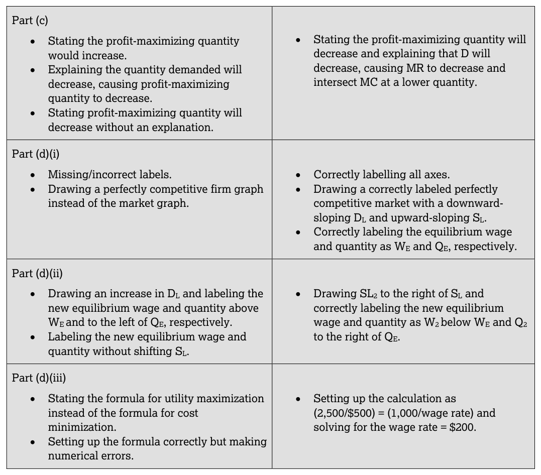

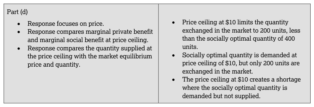
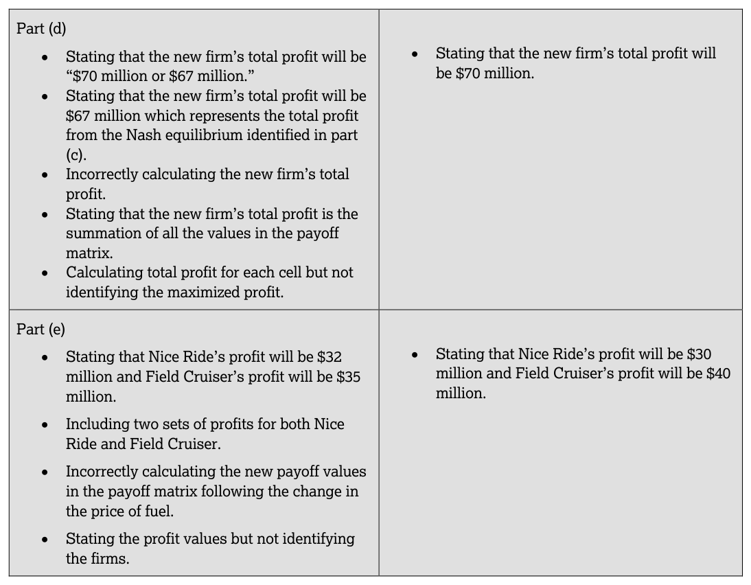
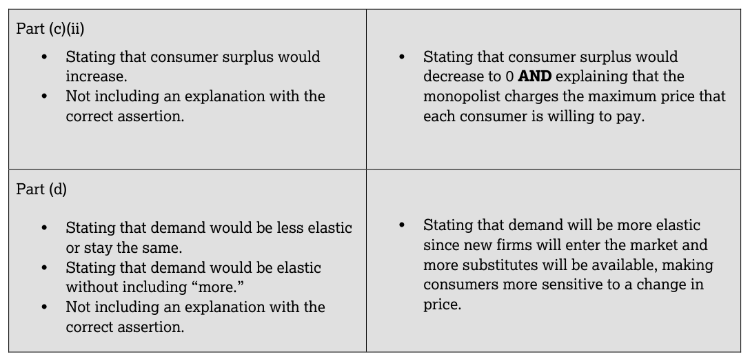
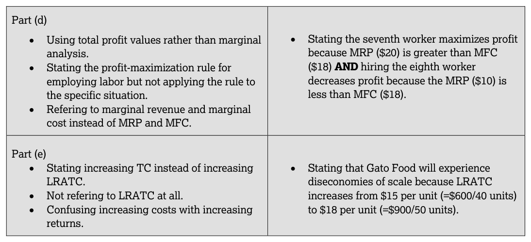
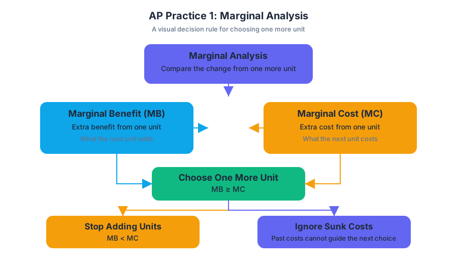
AP Practice 2
Key concepts: Consumer optimization · Constraints and trade-offs · Thinking on the margin · Price elasticity of demand · Firms’ profit-maximizing behavior · Perfect competition · Oligopoly · Game theory and normal-form models · Dominant strategies · Nash equilibrium
A sound economic decision compares the additional benefit and additional cost of an action while respecting the decision-maker’s constraints.
AP Practice 2
A sound economic decision compares the additional benefit and additional cost of an action while respecting the decision-maker’s constraints.
This original, unofficial short free-response practice combines consumer optimization, elasticity, firm behavior, perfect competition, and a simple two-player game. It is designed for approximately 12 minutes, matching the suggested time for a short Section II question. Show calculations, label every graph completely, and answer each subpart directly.
Practice prompt
A student has $30 to spend on smoothies and sandwiches. Each smoothie costs $5, and each sandwich costs $3. The student’s marginal utility schedule is:
| Quantity | Marginal utility of smoothies | Marginal utility of sandwiches |
|---|---|---|
| 1 | 40 | 24 |
| 2 | 30 | 18 |
| 3 | 20 | 12 |
| 4 | 10 | 6 |
(a) Determine the student’s utility-maximizing combination of smoothies and sandwiches. Show your reasoning using marginal utility per dollar.
The price of a smoothie increases from $5 to $6. The quantity of smoothies demanded falls from 10 to 8.
(b) Calculate the price elasticity of demand using the percentage-change definition. Classify demand as elastic or inelastic.
A perfectly competitive firm sells reusable bottles for a market price of $18. Its marginal-cost schedule is:
| Quantity | Marginal cost |
|---|---|
| 1 | $10 |
| 2 | $14 |
| 3 | $18 |
| 4 | $24 |
(c) Identify the firm’s profit-maximizing quantity. Explain why the firm does not produce the fourth unit. On a correctly labeled graph, show the firm’s demand, marginal revenue, and marginal-cost curves.
Two stores, North and South, independently decide whether to include a particular brand of shoes in a weekend sale. Their profits are shown below; the first number in each cell is North’s payoff and the second is South’s payoff.
| South: Include | South: Do not include | |
|---|---|---|
| North: Include | $(8,8)$ | $(15,5)$ |
| North: Do not include | $(5,15)$ | $(12,12)$ |
(d) Identify whether either store has a dominant strategy. Determine whether both stores choosing Do not include is a Nash equilibrium. Explain the strategic-interdependence problem represented by the game.
Worked reasoning
(a) Consumer optimization under a budget constraint
The budget constraint is the limit created by income and prices. The student should allocate spending where the marginal utility per dollar is greatest, not simply choose the item with the greatest total utility.
$$ \frac{MU_{\text{smoothie}}}{P_{\text{smoothie}}} \qquad \text{and} \qquad \frac{MU_{\text{sandwich}}}{P_{\text{sandwich}}} $$
For the first unit, a smoothie provides $40/5 = 8$ utility units per dollar, while a sandwich provides $24/3 = 8$. For the second units, the ratios are $30/5 = 6$ and $18/3 = 6$; for the third units, they are $20/5 = 4$ and $12/3 = 4$; and for the fourth units, they are $10/5 = 2$ and $6/3 = 2$.
The student can purchase six total items with the available budget if the combination costs $30. One utility-maximizing combination is 3 smoothies and 5 sandwiches, but this costs $30 only if the student can purchase five sandwiches beyond the listed schedule. Using only the listed schedule, the highest fully supported combination is 3 smoothies and 3 sandwiches, costing $24; the remaining $6 cannot purchase another smoothie but can purchase two additional sandwiches if their marginal utilities are known. Therefore, the data are insufficient to determine a unique final bundle beyond the listed schedule.
Examiner-rewarded reasoning: identify the constraint, calculate marginal utility per dollar, compare the ratios, and state when additional information is required. A conceptual statement such as “the student buys the goods with the most utility” is incomplete because optimization requires numerical comparison.
(b) Price elasticity of demand
Price elasticity of demand measures how responsive quantity demanded is to a change in price:
$$ E_d = \frac{%\Delta Q_d}{%\Delta P} $$
Using the midpoint method:
$$ %\Delta Q_d = \frac{8-10}{(8+10)/2} = \frac{-2}{9} \approx -0.222 $$
$$ %\Delta P = \frac{6-5}{(6+5)/2} = \frac{1}{5.5} \approx 0.182 $$
$$ E_d = \frac{-0.222}{0.182} \approx -1.22 $$
The absolute value is approximately $1.22$, so demand is elastic. The negative sign reflects the law of demand; classification uses the absolute value.
(c) Perfectly competitive firm
A perfectly competitive firm is a price taker, so its demand and marginal-revenue curves are horizontal at the market price:
$$ P = MR = $18 $$
The firm produces 3 units, where $MC = MR = $18$. The fourth unit is not produced because its marginal cost, $24$, exceeds the marginal revenue, $18$; producing it would reduce profit.
The graph should include a vertical axis labeled price, cost, and revenue; a horizontal axis labeled quantity; a horizontal curve labeled $d = MR = P = $18$; an upward-sloping $MC$ curve; and the profit-maximizing quantity $Q^* = 3$ where $MC$ intersects $MR$.
(d) Strategy and equilibrium
A dominant strategy is an action that produces a higher payoff regardless of the other player’s action. North should choose Include: if South includes, North earns $8 rather than $5; if South does not include, North earns $15 rather than $12. Thus, Include is North’s dominant strategy. By symmetry, Include is also South’s dominant strategy.
Both stores choosing Do not include is not a Nash equilibrium. At $(12,12)$, either store could switch alone to Include and raise its payoff from $12$ to $15. The Nash equilibrium is $(\text{Include},\text{Include})$, because neither store benefits from changing its action unilaterally once the other includes.
This is strategic interdependence: each store’s payoff depends on its own decision and the rival’s decision. Oligopolists may struggle to achieve the monopoly outcome because each firm has an incentive to pursue its individual gain, even when mutual restraint would produce higher combined profits.
Misconception check and error review
Misconception: “A firm should produce where price equals average total cost.” Correction: profit maximization occurs where $MR = MC$; in perfect competition, this becomes $P = MR = MC$, provided the firm’s short-run production condition is satisfied.
After practicing, mark each error as concept, calculation, graph, or explanation. Redo only the missed step without looking at the solution, then write one sentence explaining why the tempting incorrect answer fails.

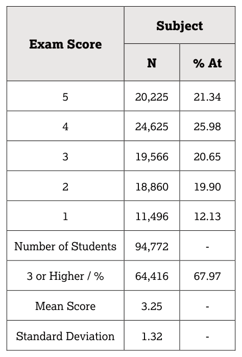
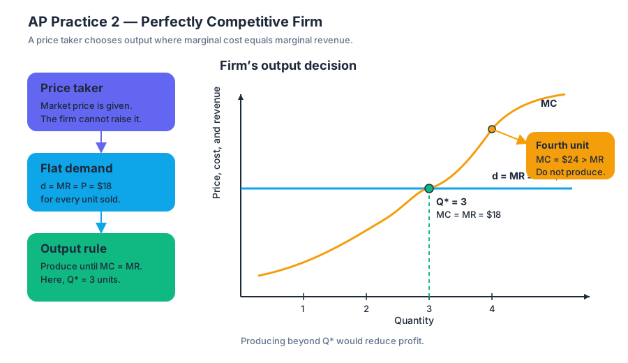
AP Practice 3
A price change does not automatically tell you whether a seller’s total revenue rises or falls; the decisive question is how strongly buyers respond. This practice task focuses on numerical analysis: calculating price elasticity of demand, interpreting its meaning, and connecting the result to total revenue.
AP Practice 3
A price change does not automatically tell you whether a seller’s total revenue rises or falls; the decisive question is how strongly buyers respond. This practice task focuses on numerical analysis: calculating price elasticity of demand, interpreting its meaning, and connecting the result to total revenue.
Task focus: numerical analysis using Skill 3: Manipulation, especially Skill 3.C, and interpretation supported by Skill 2: Interpretation. When a graph is required, use Skill 4: Graphing and Visuals, including accurate labels under Skill 4.A.
Original practice prompt
A neighborhood bakery sells boxes of specialty pastries. The bakery records the following results:
| Situation | Price per box | Quantity demanded |
|---|---|---|
| Before a price change | $8 | $500$ boxes |
| After a price change | $10 | $440$ boxes |
Answer each part using the information above.
(a) Calculate the percentage change in price and the percentage change in quantity demanded using the midpoint method.
(b) Calculate the price elasticity of demand for the bakery’s pastry boxes. State whether demand is elastic, inelastic, or unit elastic.
(c) Calculate the bakery’s total revenue before and after the price change. Did total revenue increase or decrease?
(d) Explain how the elasticity result predicts the change in total revenue.
Worked reasoning
Part (a): Calculate the percentage changes
The midpoint method uses the average of the original and new values as the denominator. This avoids choosing one endpoint as the reference point.
$$ %\Delta P= \frac{P_2-P_1}{(P_2+P_1)/2}\times 100 $$
$$ %\Delta P= \frac{10-8}{(10+8)/2}\times 100
\frac{2}{9}\times 100 \approx 22.2% $$
Quantity demanded falls from $500$ boxes to $440$ boxes:
$$ %\Delta Q_d= \frac{440-500}{(440+500)/2}\times 100 $$
$$ %\Delta Q_d= \frac{-60}{470}\times 100 \approx -12.8% $$
The negative sign matters economically: the higher price caused quantity demanded to decrease. When calculating elasticity, economists commonly use the absolute value because the law of demand normally makes price elasticity of demand negative.
Part (b): Calculate and classify elasticity
Price elasticity of demand measures the responsiveness of quantity demanded to a change in price:
$$ E_d= \left| \frac{%\Delta Q_d}{%\Delta P} \right| $$
$$ E_d= \left| \frac{-12.8%}{22.2%} \right| \approx 0.58 $$
Because $E_d<1$, demand is inelastic. Quantity demanded changes proportionally less than price. A price increase of about $22.2%$ produces a quantity decrease of only about $12.8%$.
Examiner-rewarded conclusion: The numerical calculation must be followed by the classification. Writing only “$0.58$” does not fully communicate the economic meaning.
Part (c): Calculate total revenue
Total revenue is the money received by the seller:
$$ TR=P\times Q $$
Before the price change:
$$ TR_1=$8\times 500=$4{,}000 $$
After the price change:
$$ TR_2=$10\times 440=$4{,}400 $$
Total revenue increases by:
$$ $4{,}400-$4{,}000=$400 $$
The bakery’s total revenue rises even though it sells fewer boxes.
Part (d): Explain the connection
Demand is inelastic, so the percentage decrease in quantity demanded is smaller than the percentage increase in price. The higher price therefore more than offsets the loss of sales volume, causing total revenue to increase.
What the response must show
| Required move | Strong response |
|---|---|
| Numerical manipulation | Correctly computes both midpoint percentage changes |
| Classification | Identifies $E_d\approx 0.58$ as inelastic |
| Revenue calculation | Uses $TR=P\times Q$ for both situations |
| Economic explanation | Connects inelastic demand to increased total revenue |
| Interpretation | Explains what the number means, not merely what it equals |
This is Skill 3: Manipulation because the situation requires calculations that determine an economic outcome. It also uses Skill 2: Interpretation because the numerical result must be translated into an explanation about buyer responsiveness and seller revenue.
Misconception check
Named misconception: “A price increase always lowers total revenue.”
A price increase lowers quantity demanded, but it does not necessarily lower total revenue. With inelastic demand, quantity falls by a smaller percentage than price rises, so total revenue increases. With elastic demand, quantity falls by a larger percentage, so total revenue decreases.
Another common error is reversing the elasticity ratio. Price elasticity of demand is the responsiveness of quantity demanded to price, so quantity’s percentage change belongs in the numerator:
Timing and error review
For a short numerical-analysis response, aim to complete the calculation and explanation in approximately 8–10 minutes. Reserve the final minute to check signs, midpoint denominators, units, arithmetic, and whether every numerical answer has an accompanying economic interpretation.
Afterward, classify the error rather than merely marking the answer wrong:
- Setup error: the formula or numerator/denominator was incorrect.
- Arithmetic error: the correct method produced an incorrect number.
- Classification error: the value was not compared with $1$ correctly.
- Reasoning error: the calculation was correct, but the revenue explanation was missing or contradicted the elasticity result.
Retrieval check: If the bakery’s demand had instead been elastic, with $E_d>1$, what would you predict about total revenue after the same price increase? Explain your prediction in one sentence using percentage changes, not just the words “elastic” or “inelastic.”

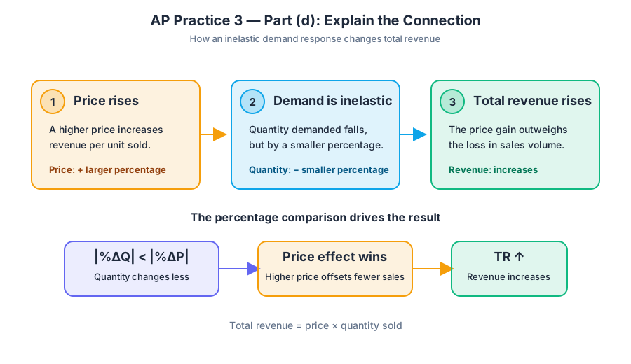
AP Practice 4
A market can produce a quantity that buyers and sellers willingly accept while still wasting potential gains from trade. A per-unit tax reveals the difference: the price paid by consumers, the price received by producers, government revenue, and deadweight loss all appear in one supply-and-demand diagram.
AP Practice 4
A market can produce a quantity that buyers and sellers willingly accept while still wasting potential gains from trade. A per-unit tax reveals the difference: the price paid by consumers, the price received by producers, government revenue, and deadweight loss all appear in one supply-and-demand diagram.
Task type: Free-response graphing and visual analysis
This original, unofficial practice focuses on Skill 4: Graphing and Visuals, while also requiring Skill 2: Interpretation and Skill 3: Manipulation. On the current hybrid AP Microeconomics Exam, free-response questions are displayed in Bluebook and answered by hand in paper booklets. A strong response does more than draw a recognizable graph: it uses labels, numerical relationships, and written economic reasoning to make the graph communicate the entire argument.
Original practice prompt
The market for reusable water bottles is initially competitive. The following linear equations describe the market, where $P$ is the price in dollars per bottle and $Q$ is the quantity of bottles per week:
$$ Q_D = 120 - 4P $$
$$ Q_S = 20 + P $$
The government imposes a tax of $$10$ on each bottle sold.
(a) Calculate the initial equilibrium price and quantity.
(b) Draw a correctly labeled graph of the market before and after the tax. Show the original equilibrium, the tax wedge, the price paid by consumers, the price received by producers, and the quantity sold after the tax.
(c) Calculate the prices paid by consumers and received by producers after the tax.
(d) Calculate the government’s tax revenue.
(e) Explain why the tax creates deadweight loss.
Worked reasoning
(a) Initial equilibrium
At equilibrium, quantity demanded equals quantity supplied:
$$ 120 - 4P = 20 + P $$
$$ 100 = 5P $$
$$ P = 20 $$
Substitute $P = 20$ into either equation:
$$ Q = 20 + 20 = 40 $$
Therefore, the initial equilibrium is:
$$ P_E = $20,\qquad Q_E = 40 $$
(b) Constructing the graph
Draw a downward-sloping demand curve labeled $D$ and an upward-sloping supply curve labeled $S$. Mark the original equilibrium at $(Q=40,\ P=$20)$.
After the tax, the consumer price exceeds the producer price by exactly $$10$:
$$ P_C - P_P = $10 $$
Graphically, the tax creates a vertical wedge between the price paid by consumers and the price received by producers at the new quantity. The new quantity must be lower than $40$, because the tax raises the consumer price and lowers the producer price relative to the original equilibrium.
(c) Prices and quantity after the tax
Let $P_P$ represent the price received by producers. Consumers pay $P_C=P_P+10$. At the post-tax equilibrium:
$$ Q_D = 120 - 4(P_P+10) $$
$$ Q_S = 20 + P_P $$
Set the two quantities equal:
$$ 120 - 4P_P - 40 = 20 + P_P $$
$$ 60 = 5P_P $$
$$ P_P = $12 $$
Consumers pay:
$$ P_C = P_P + $10 = $22 $$
The quantity sold is:
$$ Q = 20 + 12 = 32 $$
Thus:
$$ P_C=$22,\qquad P_P=$12,\qquad Q_T=32 $$
(d) Tax revenue
Government revenue equals the tax per unit multiplied by the number of units sold:
$$ TR = t \times Q_T $$
$$ TR = $10 \times 32 = $320 $$
On the graph, tax revenue is the rectangle with height $$10$ and width $32$ bottles.
(e) Deadweight loss
The tax reduces output from $40$ to $32$. The eight units no longer traded include exchanges for which buyers’ willingness to pay exceeded sellers’ opportunity cost. Those mutually beneficial trades disappear, so total surplus falls.
Deadweight loss is the triangular area between the demand and supply curves over the units not traded:
$$ DWL=\frac{1}{2}\times(\text{tax})\times(Q_E-Q_T) $$
$$ DWL=\frac{1}{2}\times $10\times(40-32)=$40 $$
What earns credit
| Response feature | Examiner-rewarded reasoning |
|---|---|
| Graphing and Visuals — Skill 4 | Demand and supply are correctly drawn and labeled; both equilibria, prices, quantities, and the tax wedge are identifiable. |
| Manipulation — Skill 3 | Equations are rearranged accurately to calculate equilibrium, tax incidence, quantity, revenue, and deadweight loss. |
| Interpretation — Skill 2 | The response connects the reduced quantity to lost mutually beneficial trades and lower total surplus. |
| Explanation | The answer distinguishes the consumer price from the producer price rather than treating the tax as changing only one price. |
Misconception check
Misconception: “The government collects $$10$ from each consumer, so consumers bear the entire tax.” The legal assignment of a tax does not determine its economic incidence. Here, consumers pay $$22$ instead of $$20$, while producers receive $$12$ instead of $$20$; both sides bear part of the burden.
Timing and error review
Allow approximately 12 minutes: $2$ minutes to read and plan, $4$ minutes for calculations, $4$ minutes for the graph and explanation, and $2$ minutes to check labels and units. Afterward, classify every error as one of four types: equation setup, arithmetic, graph labeling, or economic explanation. Redraw the graph from memory and explain, in one sentence, why the post-tax quantity must be below the original equilibrium quantity.
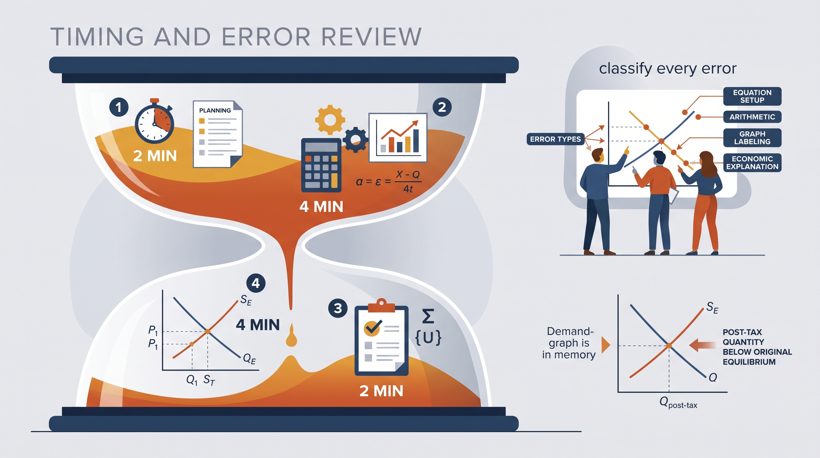
AP Practice 5
A numerical-analysis response earns more than a final number: it must expose the economic relationship that makes the number meaningful. In this practice, the central task is to use a market model to calculate equilibrium, consumer and producer surplus, and the efficiency loss created by a policy.
AP Practice 5
A numerical-analysis response earns more than a final number: it must expose the economic relationship that makes the number meaningful. In this practice, the central task is to use a market model to calculate equilibrium, consumer and producer surplus, and the efficiency loss created by a policy.
Exam task type: free-response numerical analysis, supported by interpretation and graphing. The current AP Microeconomics exam includes three free-response questions and assesses numerical analysis, economic reasoning, graphing, and written explanation. Treat the problem below as original and unofficial practice.
The market for reusable meal containers
A city’s market for reusable meal containers is described by the following equations, where $P$ is the price in dollars per container and $Q$ is the number of containers traded:
$$ Q_D = 120 - 2P $$
$$ Q_S = 20 + 2P $$
The city initially allows the market to operate without intervention. It then imposes a per-unit tax of $10$ on sellers.
Suggested timing: Spend about $12$ minutes. Reserve the final $2$ minutes to check algebra, units, graph labels, and whether each numerical answer is connected to the correct economic area.
Part A — Find the initial equilibrium
Set quantity demanded equal to quantity supplied:
$$ 120 - 2P = 20 + 2P $$
$$ 100 = 4P $$
$$ P = 25 $$
Substitute $P=25$ into either equation:
$$ Q = 120 - 2(25) = 70 $$
The initial equilibrium is therefore a price of $$25$ and a quantity of $70$ containers. A complete numerical response should include both variables and their units, not merely the algebraic value.
Reward-worthy conclusion: The market equilibrium is $\left(P,Q\right)=\left($25,70\right)$.
Part B — Calculate the initial surplus
Rewrite each curve in inverse form to identify the intercepts. Demand is:
$$ Q_D=120-2P $$
At $Q=0$:
$$ 0=120-2P \Rightarrow P=60 $$
Supply is:
$$ Q_S=20+2P $$
At $Q=0$:
$$ 0=20+2P \Rightarrow P=-10 $$
Consumer surplus is the triangular area below the demand curve and above the equilibrium price:
$$ CS=\frac{1}{2}(70)(60-25)=$1{,}225 $$
Producer surplus is the area above the supply curve and below the equilibrium price. Because the supply curve crosses the price axis at $-$10$, the relevant height is:
$$ PS=\frac{1}{2}(70)(25-(-10))=$1{,}225 $$
Thus total surplus is:
$$ TS=CS+PS=$1{,}225+$1{,}225=$2{,}450 $$
Common error — treating a negative supply intercept as impossible: A negative vertical intercept does not mean the firm pays consumers in the actual market. It is an algebraic extension of the supply curve used to calculate the area. The surplus calculation remains valid within the model.
Part C — Analyze the $10$ per-unit tax
Let $P_B$ represent the price paid by buyers. Sellers receive the buyer price minus the tax, so their net price is $P_B-10$. The after-tax supply relationship is therefore:
$$ Q_S=20+2(P_B-10) $$
$$ Q_S=2P_B $$
Set this equal to demand:
$$ 120-2P_B=2P_B $$
$$ P_B=30 $$
The quantity traded is:
$$ Q=120-2(30)=60 $$
Sellers receive:
$$ P_S=P_B-10=$20 $$
The tax raises the buyer price from $$25$ to $$30$, lowers the seller price from $$25$ to $$20$, and reduces quantity from $70$ to $60$. These three changes should appear together in a strong response because they demonstrate the tax wedge and the resulting contraction in trade.
Tax revenue equals the tax per unit multiplied by the quantity sold:
$$ TR=($10)(60)=$600 $$
After-tax consumer surplus is:
$$ CS=\frac{1}{2}(60)(60-30)=$900 $$
After-tax producer surplus is:
$$ PS=\frac{1}{2}(60)(20-(-10))=$900 $$
Total surplus including government revenue is:
$$ TS=$900+$900+$600=$2{,}400 $$
Therefore, deadweight loss is:
$$ DWL=$2{,}450-$2{,}400=$50 $$
What an examiner rewards
A high-quality numerical-analysis response does the following:
- identifies the initial equilibrium as $P=$25$ and $Q=70$;
- calculates the supply and demand intercepts before finding surplus;
- distinguishes the buyer price $P_B=$30$ from the seller price $P_S=$20$;
- calculates tax revenue using the post-tax quantity;
- includes consumer surplus, producer surplus, and government revenue in total surplus;
- identifies the deadweight loss as $$50$ and connects it to the reduction in mutually beneficial trades.
Misconception check: The tax does not eliminate all surplus, and the government’s tax revenue is not itself deadweight loss. Tax revenue is a transfer from buyers and sellers to the government; deadweight loss is the surplus from trades that no longer occur.
Error-review routine
After completing the problem, label your error as one of four types: model setup—such as shifting the wrong curve; calculation—such as solving the equilibrium incorrectly; economic interpretation—such as confusing buyer and seller prices; or presentation—such as omitting units or graph labels. Redo only the failed step, then explain in one sentence why the corrected step works.
Retrieval check: If demand were more inelastic than supply, which side would bear more of the $10$ tax? The less elastic side would bear more of the tax burden because it changes quantity less in response to the price change.
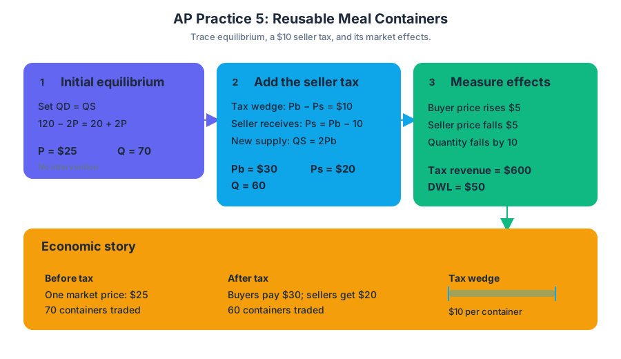
AP Practice 6
A market can produce the wrong quantity even when every buyer and seller is acting in their own interest. The exam skill is to identify the wedge between private and social incentives, represent it accurately, and explain the policy result in economic language.
AP Practice 6
A market can produce the wrong quantity even when every buyer and seller is acting in their own interest. The exam skill is to identify the wedge between private and social incentives, represent it accurately, and explain the policy result in economic language.
This original, unofficial practice uses a free-response question requiring graphing, numerical analysis, assertions, and explanations. It integrates Unit 2 supply and demand with Unit 6 market failure and the role of government.
Task profile and timing
Allocate about $12$–$15$ minutes. First identify the market mechanism, then calculate before writing explanations. For every graph, label both axes, curves, equilibrium points, and any policy-created quantities or prices. A correct idea without a readable graph or economic justification may not earn the associated point.
Original practice prompt
A city’s market for reusable delivery containers is competitive. The private marginal benefit and private marginal cost are represented by:
$$ Q_D = 120 - 2P $$
$$ Q_S = 3P $$
Production creates a constant marginal external cost of $10$ per container because cleaning and disposal impose costs on nearby residents.
(a)
Calculate the competitive equilibrium price and quantity. Show your work.
(b)
Draw a correctly labeled graph of the market. Show the demand curve, the private marginal-cost curve, the social marginal-cost curve, the market equilibrium, and the socially efficient quantity.
(c)
Calculate the socially efficient quantity.
(d)
The city imposes a per-unit corrective tax equal to the marginal external cost. Explain what happens to the market quantity and why the tax improves allocative efficiency.
(e)
Suppose demand is relatively inelastic while supply is relatively elastic. Which side of the market bears more of the tax burden? Explain.
Worked reasoning
(a) Competitive equilibrium
At equilibrium, quantity demanded equals quantity supplied:
$$ 120 - 2P = 3P $$
$$ 120 = 5P $$
$$ P = 24 $$
Substitute $P=24$ into either equation:
$$ Q = 3(24) = 72 $$
Therefore, the competitive equilibrium is $P=$24$ and $Q=72$.
Scoring target: The response must include the equilibrium condition, a correct solution for price, and a correct solution for quantity. Writing only the final coordinates does not demonstrate the required numerical reasoning as clearly as showing the equations.
(b) Market-failure graph
The supply curve represents private marginal cost, or the cost directly faced by producers. Because production creates an external cost of $10$, social marginal cost lies exactly $10$ above private marginal cost at every quantity:
$$ SMC = PMC + 10 $$
The demand curve represents marginal private benefit and, under the stated conditions, also represents marginal social benefit. The market equilibrium occurs where demand intersects $PMC$ at $(72,24)$. The efficient quantity occurs where demand intersects $SMC$.
Scoring target: A complete graph labels the vertical axis as price or cost and the horizontal axis as quantity; includes $D$, $PMC$, and $SMC$; places $SMC$ above $PMC$; identifies the market quantity $Q_M$ and efficient quantity $Q^*$; and shows the relevant intersections. A graph with curves but no labels is incomplete.
(c) Efficient quantity
Rewrite the private supply equation as an inverse supply equation:
$$ Q_S=3P $$
$$ P=\frac{Q}{3} $$
Thus:
$$ PMC=\frac{Q}{3} $$
Because the marginal external cost is $10$:
$$ SMC=\frac{Q}{3}+10 $$
Rewrite demand as inverse demand:
$$ Q_D=120-2P $$
$$ P=60-\frac{Q}{2} $$
At the efficient quantity, marginal social benefit equals social marginal cost:
$$ 60-\frac{Q}{2}=\frac{Q}{3}+10 $$
$$ 50=\frac{5Q}{6} $$
$$ Q^*=60 $$
The market produces $72$ containers, but the socially efficient quantity is $60$ containers. The market therefore overproduces by $12$ containers because producers and consumers do not fully account for the external cost.
(d) Corrective tax and efficiency
A corrective tax equal to the marginal external cost shifts the producer’s effective cost curve upward by $10$. The new market supply curve corresponds to $SMC$, so the after-tax equilibrium occurs at $Q=60$, the socially efficient quantity.
A strong explanation makes the causal chain explicit: production creates a negative externality; the market quantity is greater than the efficient quantity; the tax makes producers face the previously unpriced external cost; the supply curve shifts upward; and quantity falls from $72$ to $60$. Because the tax aligns private marginal cost with social marginal cost, the market eliminates the overproduction caused by the externality.
(e) Tax incidence
The side of the market that is relatively more inelastic bears more of the tax burden. Since demand is relatively inelastic and supply is relatively elastic, consumers bear more of the tax through a larger increase in the price they pay.
Named misconception — “The tax burden always falls on sellers.” Legal responsibility for sending the tax payment to the government does not determine economic incidence. Relative elasticity determines who can avoid the tax more easily: the less responsive side has fewer alternatives and therefore absorbs more of the burden.
Examiner-reward reasoning
| Response feature | What earns credit |
|---|---|
| Assertion | States the direction of the outcome, such as “the market overproduces.” |
| Explanation | Connects the outcome to marginal social benefit, marginal social cost, or the externality. |
| Numerical analysis | Shows equations and reaches the correct values. |
| Graphing and Visuals — Skill 4 | Uses accurate labels, correctly positioned curves, and identifiable equilibrium points. |
| Manipulation — Skill 3 | Determines how the tax changes the supply relationship and market outcome. |
Error-review routine
After completing the question, classify each error rather than merely marking it wrong:
- Model error: Did you confuse $PMC$ with $SMC$?
- Algebra error: Did you set quantity demanded equal to quantity supplied correctly?
- Graph error: Did you shift the supply curve vertically by the tax rather than moving demand?
- Explanation error: Did you state the result without explaining the marginal incentive?
- Incidence error: Did you use elasticity, or did you rely on who is legally taxed?
Retrieval check: If the external cost rose from $10$ to $15$, would the $SMC$ curve shift upward or downward, and would the efficient quantity rise or fall? The answer is upward and fall: a larger unpriced harm creates a larger gap between private and social cost, so the efficient output is lower.

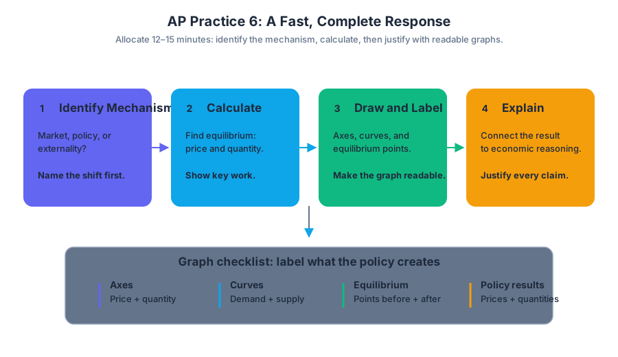
Source Materials
- AP Microeconomics Course and Exam Description
- AP Microeconomics Course and Exam Description Clarifications and Corrections
- AP Microeconomics Course Overview
- AP Microeconomics Course at a Glance
- AP Microeconomics Course at a Glance Poster
- AP Microeconomics
- AP Microeconomics
- AP Microeconomics Sample Syllabus 1
- Figure — AP Microeconomics Course and Exam Description (p. 1)
- Figure — AP Microeconomics Course and Exam Description (p. 17)
- Figure — AP Microeconomics Course and Exam Description (p. 25)
- Figure — AP Microeconomics Course and Exam Description (p. 26)
Study AP Microeconomics with AI — Free on Lykke
Sign up for free to generate personalized flashcards, quizzes, and study guides from this course. Chat with an AI tutor that knows the material.
Get Started FreeView this course wiki on Lykke · Browse all public course wikis