AP Macroeconomics
Institution: MIT
111 study materials · 49 sections
AP Macroeconomics students working the current College Board Course and Exam Description, including first-time students with no prior background, plus teachers reviewing the page for CED alignment.; Teach every official CED unit and every numbered topic at topic granularity.; Develop every AP skill / science-practice code explicitly and by name.; Replace description with teaching: worked contextual examples, named misconceptions, and in-flow retrieval checks.; Build an exam-practice unit covering every task type on the current exam.
Course Sections
Course Framework, Skills and Reasoning Processes
Key concepts: AP course framework · Economics skills · Principles and models · Quantitative analysis · Graphing and visual interpretation · Markets and equilibrium · Macroeconomic measurements and changes · Economic policy · College-level course expectations · Curriculum and instructional resources
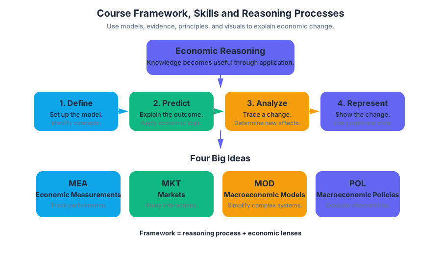
Macroeconomics becomes powerful when a student can move through four steps: define the model, explain what it predicts, determine how a change alters the outcome, and represent that change accurately.
Course Framework, Skills and Reasoning Processes
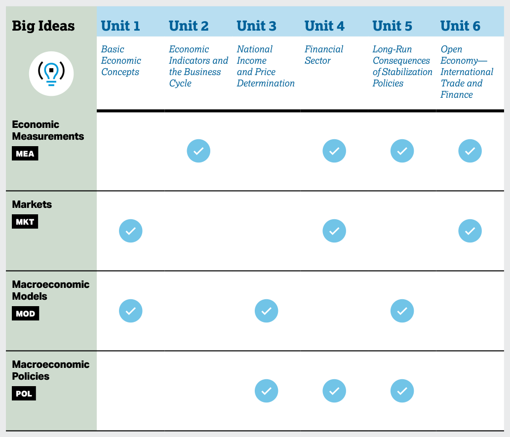
Macroeconomics becomes powerful when a student can move through four steps: define the model, explain what it predicts, determine how a change alters the outcome, and represent that change accurately. The AP Macroeconomics framework organizes this reasoning around four skill categories and four recurring Big Ideas: MEA: Economic Measurements, MKT: Markets, MOD: Macroeconomic Models, and POL: Macroeconomic Policies.
Core principle: Economic knowledge is not only knowing that a concept exists; it is using principles, models, quantitative evidence, and visual representations to explain what happens in an economy.
The framework is a guide, not a curriculum
The Course and Exam Description provides a clear, detailed description of required course content and skills, but it is not a curriculum. A college-level macroeconomics textbook should supply the substantive explanations and examples, while teachers create the instructional sequence, activities, and learning experiences.
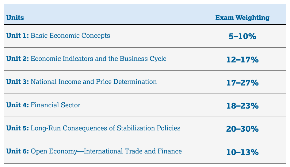
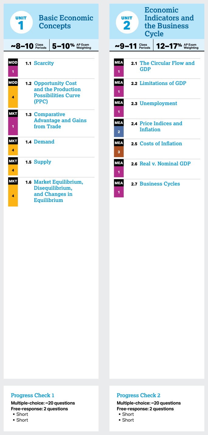
The six-unit sequence shown in the publication is therefore optional rather than mandatory. Its value is organizational: it shows how topics, Big Ideas, skills, suggested pacing, and AP Exam weighting fit together. The framework also emphasizes spiraling: students repeatedly use the same skills in increasingly complex settings, from scarcity and markets to monetary policy, economic growth, and international finance.
| Big Idea | Central concern | Typical application |
|---|---|---|
| MEA: Economic Measurements | How economic activity is measured | GDP, unemployment, inflation, real versus nominal values |
| MKT: Markets | How buyers, sellers, and financial participants interact | Equilibrium, disequilibrium, exchange rates, loanable funds |
| MOD: Macroeconomic Models | How simplified models explain economy-wide relationships | PPC, AD–AS, money market, Phillips curve |
| POL: Macroeconomic Policies | How government and central-bank actions affect outcomes | Fiscal policy, monetary policy, automatic stabilizers |
The four AP Economics Skills
The AP Economics skills describe what students should be able to do while exploring course concepts. The categories are progressive, but they are not a rigid ladder: a single response may require definition, causal explanation, calculation, and graphing together.
Skill Category 1: Principles and Models
1.A: Define economic principles and models. A response might define scarcity, aggregate demand, or the natural rate of unemployment precisely enough to distinguish it from a related idea.
1.B: Identify economic principles, models, and outcomes. Identification means recognizing which model or principle applies. For example, a question involving planned investment and interest rates points toward the loanable funds market, not the market for goods and services.
Skill Category 2: Interpretation
2.A: Explain economic outcomes. Explanation requires a causal chain, not a restatement. If consumer confidence falls, a strong explanation is: consumption decreases, aggregate demand shifts left, real output falls in the short run, and the price level decreases, assuming other factors remain constant.
2.B: Explain the effect of a change in an economic situation. This skill asks students to connect a changed condition to its consequences across a model or market. A higher reserve requirement, for instance, can reduce banks’ ability to create deposits and decrease the money supply.
2.C: Interpret a specific economic outcome using quantitative data or calculations. Students must explain what a number means economically. If nominal GDP rises from $500 billion to $525 billion, the increase is $25 billion, or $25 billion divided by $500 billion, which equals $5%$; that does not prove real production increased because prices may also have risen.
Skill Category 3: Manipulation
3.A: Determine the outcome of an economic situation using economic concepts, principles, or models. This is prediction through a model: identify the shock, select the correct curve or relationship, and state the resulting change in an economic variable.
3.B: Determine the effect(s) of one or more changes on other economic markets. Macroeconomic events often cross markets. Expansionary fiscal policy can raise aggregate demand, increase the budget deficit, increase demand for loanable funds, raise the real interest rate, and reduce private investment through crowding out.
3.C: Determine the effect of a change in an economic situation using quantitative data or calculations. For a government-spending multiplier, students may use $1/(1-\text{MPC})$. With an MPC of $0.75$, the multiplier is $1/0.25=4$; an increase in government spending of $10$ produces a maximum change in real GDP of $4 \times $10=$40$.
Skill Category 4: Graphing and Visuals
4.A: Draw an accurately labeled graph or visual to represent an economic model or market. Axes, curve names, equilibrium points, and relevant variables are not decoration: they establish whether the model is being used correctly.
4.B: Demonstrate your understanding of a specific economic situation on an accurately labeled graph or visual. The graph must show the initial condition and locate the outcome, such as equilibrium output and the price level in an AD–AS model.
4.C: Demonstrate the effect of a change in an economic situation on an accurately labeled graph or visual. A complete response shows the directional movement—such as $AD_1$ shifting to $AD_2$—and identifies the resulting changes in output, unemployment, or the price level.
How the skills appear on the exam
The multiple-choice section—$60$ questions in $70$ minutes—can test any combination of the four categories through definitions, calculations, data interpretation, model-based predictions, and graphs. The free-response section contains one long question and two short questions in $60$ minutes; it particularly rewards clear assertions, causal explanations, numerical analysis, and accurately labeled graphs.
A reliable response pattern is:
- Name the relevant principle or model.
- State the direction of the change.
- Explain the causal mechanism.
- Calculate when numerical evidence is provided.
- Graph the initial and changed equilibrium when requested.
- Connect the graph or calculation back to the specific economic outcome.
Misconception check: A graph alone is not an explanation. Saying “$AD$ shifts left” earns less reasoning value than identifying the cause—such as lower consumer spending—and linking it to lower real output and a lower price level in the short run.
Retrieval check
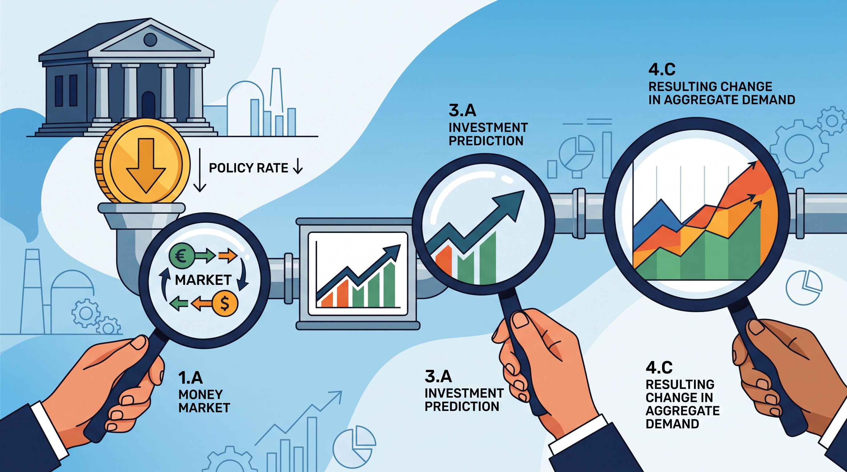
A central bank lowers its policy interest rate. Which skill is used when you define the money market, which is used when you predict the effect on investment, and which is used when you draw the resulting change? The strongest answer uses 1.A, 3.A, and 4.C, then explains the transmission from the interest rate to investment and aggregate demand.



1.1 Scarcity
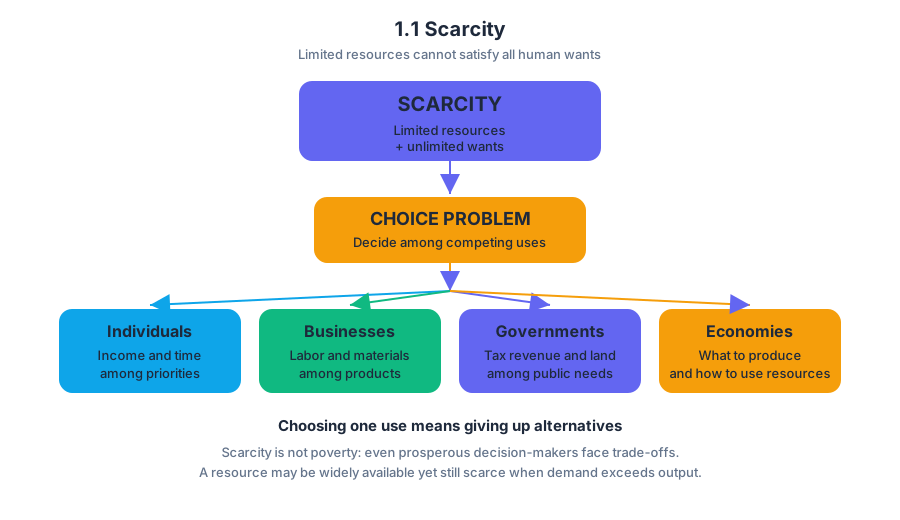
Every economy faces scarcity because the resources used to produce goods and services are limited, while human wants are effectively unlimited. Scarcity is not the same as poverty: even a wealthy household, successful business, or prosperous government must decide how to use limited time, money, workers, land, and…
1.1 Scarcity
Every economy faces scarcity because the resources used to produce goods and services are limited, while human wants are effectively unlimited. Scarcity is not the same as poverty: even a wealthy household, successful business, or prosperous government must decide how to use limited time, money, workers, land, and equipment among competing purposes.
Scarcity is the condition in which limited resources cannot satisfy all human wants.
The central economic problem is therefore a choice problem. If a city has one vacant parcel of land, it cannot simultaneously use that exact parcel for a school, a hospital, apartments, and a park. If a student has two hours before an exam, those hours cannot be fully devoted to studying, working, sleeping, and socializing at the same time. Choosing one use means giving up at least one alternative.
Scarcity operates at every level of economic decision-making:
- Individuals and households allocate limited income and time.
- Businesses allocate limited labor, raw materials, machinery, and financial resources.
- Governments allocate limited tax revenue, public workers, land, and administrative capacity.
- Entire economies must decide which goods and services to produce and how to use available resources.
The existence of scarcity does not mean that every item is rare in an absolute sense. A product can be widely available and still be scarce if people want more of it than can be produced with current resources. Scarcity is about the relationship between available resources and desired uses, not merely about whether an object exists.
Scarcity creates economic choices
Suppose a coastal town has enough construction workers and materials to complete only one major project this year. Residents want both a flood barrier and a new community health center. The resources are scarce relative to the town’s competing wants, so the town must choose. Building the flood barrier may protect homes and businesses; building the health center may improve access to medical care. The economic issue is not whether either project is desirable. Both are desirable. The issue is that the town cannot undertake both with the resources currently available.
A choice is necessary whenever resources have alternative uses. Alternative uses are the different purposes to which a resource could be devoted. A worker can produce one type of good during a particular hour; a building can house one activity at a time; a government dollar can fund one program rather than another. Scarcity makes prioritization unavoidable.
Key chain:
Limited resources $\rightarrow$ competing uses $\rightarrow$ necessary choices.
The next economic question is what is sacrificed by a choice. That sacrifice is called opportunity cost, developed formally with the Production Possibilities Curve in Topic 1.2. Scarcity is the condition that makes opportunity cost unavoidable; it does not itself identify the specific alternative sacrificed.
Scarcity versus shortage
A shortage is a situation in which quantity demanded exceeds quantity supplied at a particular price. A shortage may be temporary—for example, when a sudden storm disrupts deliveries—or persistent if the price remains below the market-clearing level or if production remains constrained.
Scarcity and shortage are related but distinct:
| Concept | Meaning | Example |
|---|---|---|
| Scarcity | Resources are insufficient to satisfy all wants. | Limited urban land must serve housing, transportation, and recreation. |
| Shortage | At a particular price, buyers want more than sellers offer. | At a legally fixed low price, more renters seek apartments than landlords provide. |
A shortage can exist for one good while scarcity exists throughout the economy. Conversely, a scarce good does not automatically produce a shortage: if its price adjusts so that quantity demanded equals quantity supplied, the market may have no shortage at that moment. Scarcity is fundamental and unavoidable; a shortage is a market condition connected to a particular price.
Worked example: choosing under scarcity
A school has $10{,}000$ available for one improvement. It can purchase laboratory equipment, repair athletic facilities, or upgrade classroom technology. Because the budget is limited and all three projects are valued, the school faces scarcity.
To reason correctly:
- The scarce resource is the school’s $10{,}000$ budget.
- The competing wants are laboratory equipment, athletic repairs, and classroom technology.
- The necessary choice is which project receives the funds.
- The chosen project uses resources that cannot simultaneously be used for the other projects.
- The best rejected alternative becomes relevant as the opportunity cost.
Named misconception — “Scarcity means nobody can obtain the good.” Incorrect. Scarcity means that available resources cannot satisfy every desired use. People may still obtain the good, but choices, trade-offs, and possibly prices determine who receives it and how much is available.
Application check: A hospital has only one intensive-care bed available, while two patients need it. Identify the scarce resource, the competing wants, and the choice that scarcity requires. Then state why the situation illustrates scarcity even if the hospital is otherwise well funded.
Retrieval check: A store has plenty of coffee in stock, but at its current low price customers want more coffee than the store offers. Is this primarily an example of scarcity, a shortage, or both? Explain the distinction in one sentence.

1.2 Opportunity Cost and the Production Possibilities Curve (PPC)
Key concepts: Scarcity and choice · Opportunity cost · Production possibilities curve (PPC) · Efficiency and underutilized resources · Economic growth and contraction · PPC shifts · Opportunity-cost patterns and PPC shape · Full and efficient use of resources
A production possibilities curve (PPC) shows the maximum combinations of two goods or activities that an economy can produce with its available resources and technology.
1.2 Opportunity Cost and the Production Possibilities Curve (PPC)
A production possibilities curve (PPC) shows the maximum combinations of two goods or activities that an economy can produce with its available resources and technology. Its central question is simple: If more of one activity is chosen, what must be given up?
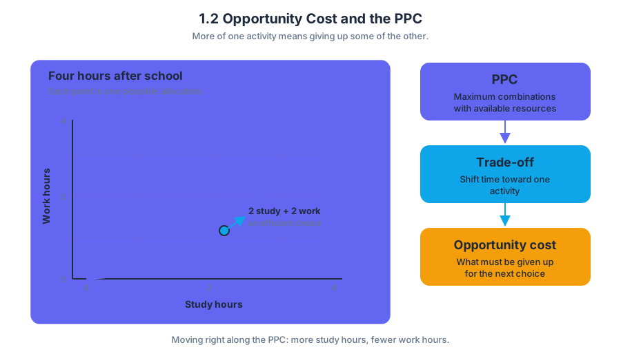
Imagine that you have four hours after school and must divide them between studying and working at a café. Every hour shifted toward one activity is an hour unavailable for the other. The PPC turns that everyday trade-off into a graph: one axis measures study hours, the other measures work hours, and each point represents one possible allocation.
Reading a PPC: trade-offs, efficiency, and feasibility
The PPC model demonstrates the trade-offs associated with allocating scarce resources. A trade-off is the act of giving up one option to obtain another. Opportunity cost is the value of the next-best alternative forgone; on a PPC, it is the amount of one good sacrificed to produce more of the other.
A point on the curve represents productive efficiency: resources are being used fully and appropriately given current technology. A point inside the curve is feasible but inefficient because some resources are unemployed, underutilized, or poorly allocated. A point outside the curve is unattainable with the economy’s current resources and technology.
Scenario check: An economy’s PPC connects a maximum of $40$ medical devices and $0$ tons of food with a maximum of $0$ medical devices and $100$ tons of food. Classify a combination of $20$ medical devices and $50$ tons of food if it lies below the curve, a combination lying exactly on the curve, and a combination above the curve. The first is feasible but inefficient, the second is productively efficient, and the third is currently unattainable—not automatically “better.”
Worked example: calculating opportunity cost
Suppose four hours can be allocated between studying and working. The available combinations are:
| Study hours | Work hours |
|---|---|
| $0$ | $4$ |
| $1$ | $3$ |
| $2$ | $2$ |
| $3$ | $1$ |
| $4$ | $0$ |
Moving from $1$ hour of studying to $2$ hours increases study time by $1$ hour but reduces work time from $3$ hours to $2$ hours. Therefore, the opportunity cost of that additional hour of studying is $1$ hour of work. Moving from $0$ to $4$ study hours gives up all $4$ work hours, so the total opportunity cost of $4$ study hours is $4$ work hours.
If every additional study hour always costs exactly $1$ work hour, the PPC is a straight line and opportunity cost is constant. If the work sacrificed rises as more study is produced, the PPC is bowed outward and opportunity cost is increasing. If the sacrificed work falls as more study is produced, opportunity cost is decreasing, producing a bowed-inward curve.
Movements along the curve versus shifts
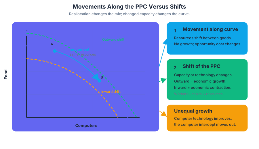
A movement along a PPC occurs when resources are reallocated between the two goods while the economy’s resources and technology remain unchanged. It does not represent economic growth; it represents a different efficient combination and therefore a different opportunity cost.
A shift changes the economy’s production possibilities. More workers, additional capital, improved natural resources, or better productivity and technology can shift the PPC outward. An outward shift represents economic growth, because more of at least one good—and usually more of both—can be produced. Destruction of factories, loss of workers, reduced resources, or technological damage can shift the PPC inward and represent economic contraction.
Growth need not expand both axes equally. A technological improvement used only to produce computers may move the computer intercept outward while leaving the maximum possible food output unchanged. The correct graph therefore depends on which resource or technology changed.
Misconception check
Misconception: “Every point inside the PPC is impossible.” It is the opposite: an interior point is attainable, but it does not use available resources efficiently. Misconception: “A point outside the PPC proves the economy is inefficient.” An outside point cannot currently be produced; inefficiency is shown by an attainable point inside the curve. Misconception: “More of one good means the PPC shifted.” More production caused by reallocating existing resources is a movement along the curve; a shift requires changed resources, technology, or productivity.
AP traceability in action
The required work appears in Learning Objective MOD-1.B.a, “Define (using graphs as appropriate) the PPC and related terms,” MOD-1.B.b, which asks students to explain how the PPC illustrates opportunity costs, trade-offs, inefficiency, efficiency, and economic growth or contraction, and MOD-1.B.c, which asks students to calculate opportunity cost using PPC or table data. These objectives are grounded in MOD-1.B.1 through MOD-1.B.5: trade-offs, the PPC’s applications, its shape, its shifts, and outward movement from economic growth.
The associated skill is Skill Category 4: Graphing and Visuals, especially 4.A, “Draw an accurately labeled graph or visual.” On an exam, label both axes, identify the curve, mark relevant points, and show a shift with a new curve rather than an arrow alone. For calculations, write the change in the sacrificed good over the change in the chosen good: $\text{opportunity cost}=\frac{\Delta\text{good forgone}}{\Delta\text{good gained}}$.
Retrieval check
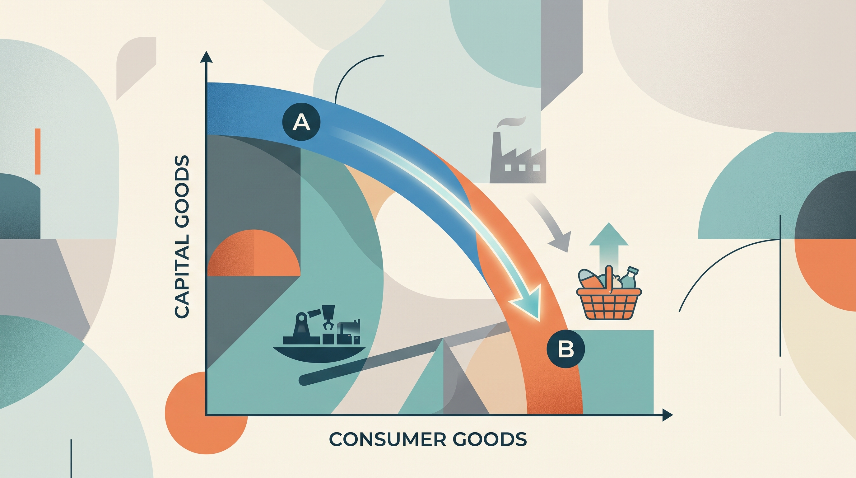
A country moves from one point on an unchanged PPC to another point with more consumer goods and fewer capital goods. Is this a shift or a movement, and what happens to the opportunity cost of the consumer goods? Answer: It is a movement along the PPC; calculate the capital goods forgone per additional consumer good to determine the opportunity cost. A shift would require a change in resources, technology, or productivity.

1.3 Comparative Advantage and Gains from Trade
Key concepts: Absolute advantage · Comparative advantage · Opportunity cost · Production possibility curves (PPCs) · Specialization according to comparative advantage · Gains from trade · Exchange opportunities · Mutually beneficial terms of trade · Consumption opportunities beyond specialization · Tradeoffs and full employment
A producer can benefit from trade even when another producer is better at making everything. The key question is not “Who produces more?” but “Who gives up less to produce this good?”
1.3 Comparative Advantage and Gains from Trade
A producer can benefit from trade even when another producer is better at making everything. The key question is not “Who produces more?” but “Who gives up less to produce this good?”
MKT-1: Production and consumption increase by engaging in trade.
Absolute advantage versus comparative advantage
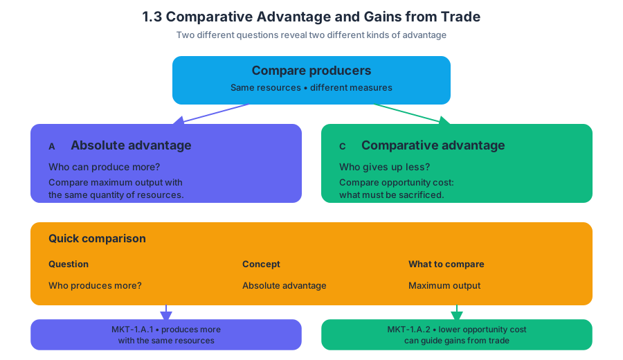
Absolute advantage means the ability of an individual, business, or country to produce more of a good or service than another producer using the same quantity of resources. It is a comparison of productivity.
Comparative advantage means the ability to produce a good or service at a lower opportunity cost than another producer. It is a comparison of what must be sacrificed.
These ideas answer different questions:
| Question | Concept | What to compare |
|---|---|---|
| Who can produce more? | Absolute advantage | Maximum output |
| Who gives up less of another good? | Comparative advantage | Opportunity cost |
The official knowledge chain is MKT-1.A.1, which defines absolute advantage as producing more with the same resources, and MKT-1.A.2, which defines comparative advantage as producing at a lower opportunity cost. A producer may have absolute advantage in both goods but comparative advantage in only one.
Finding advantage from a production table
Suppose two countries use the same resources to produce wheat and cloth:
| Country | Maximum wheat | Maximum cloth |
|---|---|---|
| Aurora | $10$ units | $5$ units |
| Borealis | $6$ units | $12$ units |
Aurora has the absolute advantage in wheat because $10>6$. Borealis has the absolute advantage in cloth because $12>5$.
To find comparative advantage, calculate opportunity costs. If each country’s production possibilities curve is linear, the opportunity cost of one unit of wheat is:
$$ \text{Opportunity cost of 1 wheat}
\frac{\text{maximum cloth}}{\text{maximum wheat}} $$
For Aurora:
$$ \text{OC}_{A}(1\text{ wheat})=\frac{5\text{ cloth}}{10\text{ wheat}}=0.5\text{ cloth} $$
For Borealis:
$$ \text{OC}_{B}(1\text{ wheat})=\frac{12\text{ cloth}}{6\text{ wheat}}=2\text{ cloth} $$
Aurora gives up less cloth when producing wheat, so Aurora has the comparative advantage in wheat. Borealis has the comparative advantage in cloth because its opportunity cost of cloth is lower:
$$ \text{OC}_{A}(1\text{ cloth})=2\text{ wheat} $$
$$ \text{OC}_{B}(1\text{ cloth})=0.5\text{ wheat} $$
Specialization and gains from trade
Specialization according to comparative advantage means each producer concentrates resources on the good it can produce at the lower opportunity cost. Aurora specializes in wheat, while Borealis specializes in cloth.
Before specialization, suppose Aurora produces $6$ wheat and $2$ cloth, while Borealis produces $3$ wheat and $6$ cloth. Total production is:
$$ 9\text{ wheat}+8\text{ cloth} $$
After specialization, Aurora produces $10$ wheat and Borealis produces $12$ cloth. Total production becomes:
$$ 10\text{ wheat}+12\text{ cloth} $$
Specialization increases total production because resources move toward their relatively most productive uses. Trade then allows the countries to share those gains.
Mutually beneficial terms of trade
Terms of trade are the rate at which one good exchanges for another. For both countries to benefit, the exchange rate must fall between their opportunity costs.
For one unit of wheat:
$$ 0.5\text{ cloth}<\text{terms of trade}<2\text{ cloth} $$
Choose the terms of trade of $1$ wheat for $1$ cloth. Aurora specializes in $10$ wheat and trades $4$ wheat for $4$ cloth. Borealis specializes in $12$ cloth and receives $4$ wheat in exchange for $4$ cloth.
Final consumption:
- Aurora: $6$ wheat and $4$ cloth
- Borealis: $4$ wheat and $8$ cloth
Both consumption bundles lie beyond what each country could produce alone on its own PPC. Aurora could not produce $6$ wheat and $4$ cloth domestically, and Borealis could not produce $4$ wheat and $8$ cloth domestically. This is MKT-1.B.1: specialization creates exchange opportunities that expand consumption beyond the PPC.
The trade rate is mutually beneficial because $1$ wheat costs Aurora more than $0.5$ cloth but less than $2$ cloth—the sacrifices faced by the two countries. This is MKT-1.B.2: comparative advantage and opportunity costs determine mutually beneficial terms of trade.
Common misconception
Misconception: Absolute advantage determines specialization.
Correction: Absolute advantage identifies who can produce more. Comparative advantage determines who should specialize. Even a country with absolute advantage in both goods should specialize in the good with the lower opportunity cost.
AP skills in action
This topic develops Skill Category 1: Principles and Models, especially 1.A Define economic principles and models and 1.B Explain economic principles and models. It also uses Skill Category 3: Manipulation, particularly calculating opportunity costs and mutually beneficial terms of trade from tables or PPC data, and Skill Category 4: Graphing and Visuals when students identify full-employment production points and consumption beyond a PPC.
MKT-1.B requires students to explain how comparative-advantage specialization and appropriate terms of trade create gains from trade, and to calculate mutually beneficial terms of trade.
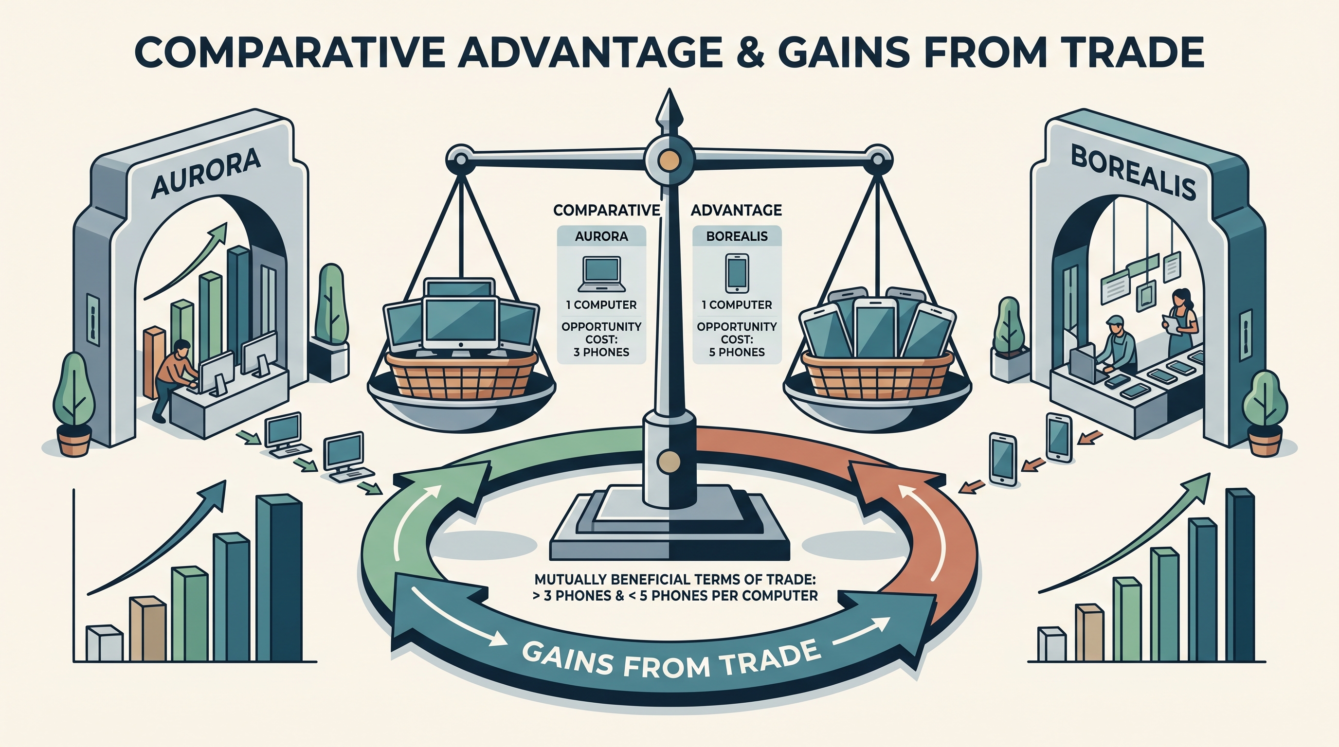
Retrieval check: Aurora’s opportunity cost of one computer is $3$ phones, while Borealis’s is $5$ phones. Who has comparative advantage in computers, and what range of terms of trade for one computer could benefit both producers?
Answer: Aurora has comparative advantage in computers. Mutually beneficial terms of trade must be greater than $3$ phones but less than $5$ phones per computer.
1.4 Demand
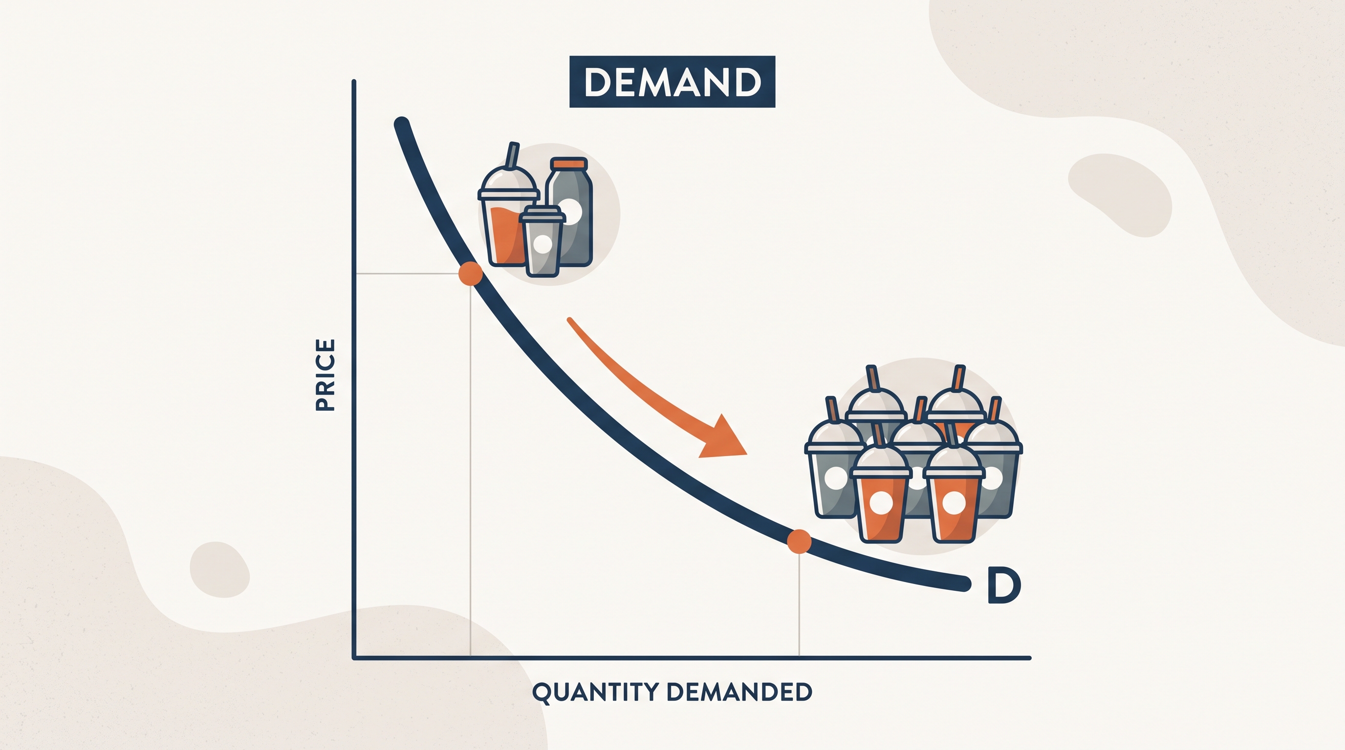
When the price of a product changes, buyers usually change how much they want to purchase—even if nothing else about the market changes. Demand is the relationship between the price of a good or service and the quantity consumers are willing and able to buy at each possible price.
1.4 Demand
When the price of a product changes, buyers usually change how much they want to purchase—even if nothing else about the market changes. Demand is the relationship between the price of a good or service and the quantity consumers are willing and able to buy at each possible price.
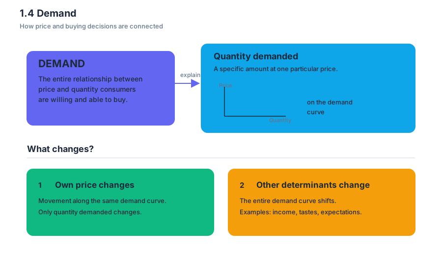
Demand is the entire relationship between price and quantity demanded. Quantity demanded is the specific amount consumers want to buy at one particular price.
The distinction matters because economists describe two different events: a change in the product’s own price causes a movement along the demand curve, while a change in any other demand determinant shifts the entire curve.
The law of demand
The law of demand states that, holding all other factors constant, price and quantity demanded move in opposite directions. When price rises, quantity demanded falls; when price falls, quantity demanded rises.
$$P \uparrow \Rightarrow Q_d \downarrow$$
$$P \downarrow \Rightarrow Q_d \uparrow$$
A downward-sloping demand curve represents this inverse relationship. The vertical axis measures price, $P$, and the horizontal axis measures quantity, $Q$. Each point on the curve gives the quantity demanded at one price.
Worked example — concert tickets: Suppose the number of tickets demanded is represented by
$$Q_d = 1{,}200 - 40P$$
where $P$ is the ticket price in dollars. At $P=$10$,
$$Q_d = 1{,}200 - 40(10)=800$$
At $P=$15$,
$$Q_d = 1{,}200 - 40(15)=600$$
The price rises by $$5$, and quantity demanded falls by $200$ tickets. This is a movement upward and to the left along the same demand curve.
The law of demand is connected to the idea of opportunity cost: a higher price makes the purchase more costly relative to other uses of a buyer’s limited income. Buyers may switch toward alternatives, and the higher price may also reduce the amount they can afford.
Changes in demand versus changes in quantity demanded
A change in quantity demanded occurs only when the good’s own price changes. The demand curve does not move.
A change in demand occurs when a nonprice determinant changes. The entire demand curve shifts.
| Event | Graphical result | Typical example |
|---|---|---|
| Price of the good changes | Movement along demand curve | The price of coffee falls |
| Income changes | Demand curve shifts | Household incomes rise |
| Price of a related good changes | Demand curve shifts | Tea becomes more expensive |
| Preferences change | Demand curve shifts | A health trend increases interest in fruit |
| Number of buyers changes | Demand curve shifts | More consumers enter the market |
| Expected future price changes | Demand curve shifts | Buyers expect prices to rise next month |
A shift right means an increase in demand: consumers want more at every possible price. A shift left means a decrease in demand: consumers want less at every possible price.
The determinants of demand
The principal determinants of demand are tastes and preferences, the number of buyers, consumer income, the prices of related goods, and expectations about the future.
For normal goods, an increase in income increases demand. For example, if incomes rise, consumers may purchase more restaurant meals at every restaurant price. For an inferior good, an increase in income decreases demand because consumers move toward preferred alternatives; bus rides can serve as a possible example if consumers switch to cars or ride-sharing as their incomes increase.
Substitutes are goods that can be used in place of one another. If the price of tea rises, demand for coffee may increase because coffee becomes relatively more attractive. Complements are goods used together. If the price of printers falls, demand for printer ink may increase because consumers are more likely to purchase and use printers.
Expectations can change current demand. If buyers expect a product’s price to rise soon, they may purchase more today, shifting current demand right. If they expect a price decrease, they may postpone purchases, shifting current demand left.
Named misconception check
Misconception: “If demand increases, the price must have increased.” Correction: an increase in demand is a rightward shift caused by a nonprice determinant. A price increase causes a decrease in quantity demanded—a movement along the existing curve—not an increase in demand.
Misconception: “Demand is the same as desire.” Correction: demand requires both willingness and ability to buy. Someone may want a luxury home but lack the income to participate in that market at the listed price.
AP traceability and retrieval check
Topic 1.4 Demand develops Big Idea MKT (Markets). Its core identifiers are LO MKT-1.A and EK MKT-1.A.1–MKT-1.A.2 for the law of demand, LO MKT-1.B and EK MKT-1.B.1 for determinants of demand, and LO MKT-1.C and EK MKT-1.C.1 for distinguishing movements along a demand curve from shifts of the curve. The principal assessed processes are Skill 1.A: Define economic principles and models, Skill 1.B: Explain economic outcomes, Skill 2.C: Interpret visual representations, and Skill 4.A: Draw correctly labeled graphs.
Retrieval check: The price of smoothies falls, while consumer incomes and preferences remain unchanged. Is this a movement along the demand curve or a shift? What happens to quantity demanded?
Answer: It is a movement downward along the existing demand curve, and quantity demanded increases. A shift would require a change in a nonprice determinant such as income, preferences, the number of buyers, the price of a related good, or expectations.
1.5 Supply
A bakery supplies more loaves when the selling price rises because each additional loaf becomes more rewarding to produce. Supply is the relationship between the price of a good or service and the quantity producers are willing and able to sell during a specific period, holding other relevant factors constant.
1.5 Supply
A bakery supplies more loaves when the selling price rises because each additional loaf becomes more rewarding to produce. Supply is the relationship between the price of a good or service and the quantity producers are willing and able to sell during a specific period, holding other relevant factors constant.
Law of supply: As price rises, quantity supplied generally rises; as price falls, quantity supplied generally falls, ceteris paribus—with all other conditions unchanged.
The key phrase is quantity supplied: it means the amount producers offer at one particular price. A change in the product’s own price causes a movement along the existing supply curve, not a shift of the curve.
Reading an individual supply curve
Suppose one bakery’s daily supply schedule is:
| Price per loaf | Quantity supplied |
|---|---|
| $2 | 80 loaves |
| $3 | 120 loaves |
| $4 | 160 loaves |
On a graph, price is placed on the vertical axis and quantity on the horizontal axis. The upward-sloping supply curve shows that higher prices create an incentive to produce more: the bakery may schedule extra workers, run ovens longer, or use less convenient production methods.
Price
  ^
$4|                         ●
  |                    /
$3|              ●    /
  |            /
$2|      ●    /
  |       /
  +--------------------------------> Quantity
        80       120       160
              loaves per day
If the price rises from $2 to $4, quantity supplied increases from 80 to 160 loaves per day. This is an increase in quantity supplied, represented by movement upward and to the right along the same supply curve. It is not an “increase in supply.”
Market supply: adding producers
Market supply is the total quantity supplied by all producers at each possible price. To construct it, add producers’ quantities horizontally—that is, add the quantities supplied at the same price.
At a price of $3, imagine three bakeries supply 120, 50, and 30 loaves per day. The market quantity supplied is therefore
$$ 120+50+30=200\text{ loaves per day}. $$
The unit matters: $3 is the price, while 200 loaves per day is the quantity. A quantity cannot be reported in dollars unless the question specifically asks for the value of output.
Shifts in supply
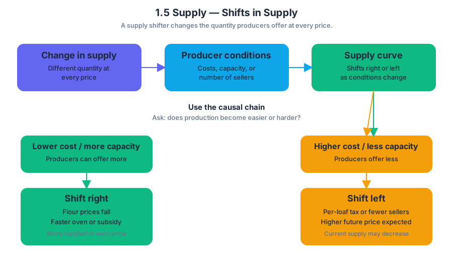
A change in supply shifts the entire supply curve because producers now offer a different quantity at every price. Factors that can shift supply include input prices, technology, taxes or subsidies, expectations, the number of sellers, and conditions affecting production.
Use the following causal chain to predict the direction of a shift:
| Change | Producer cost or capacity | Supply curve |
|---|---|---|
| Flour prices fall | Production becomes less costly | Shifts right |
| A faster oven is invented | More can be produced with the same resources | Shifts right |
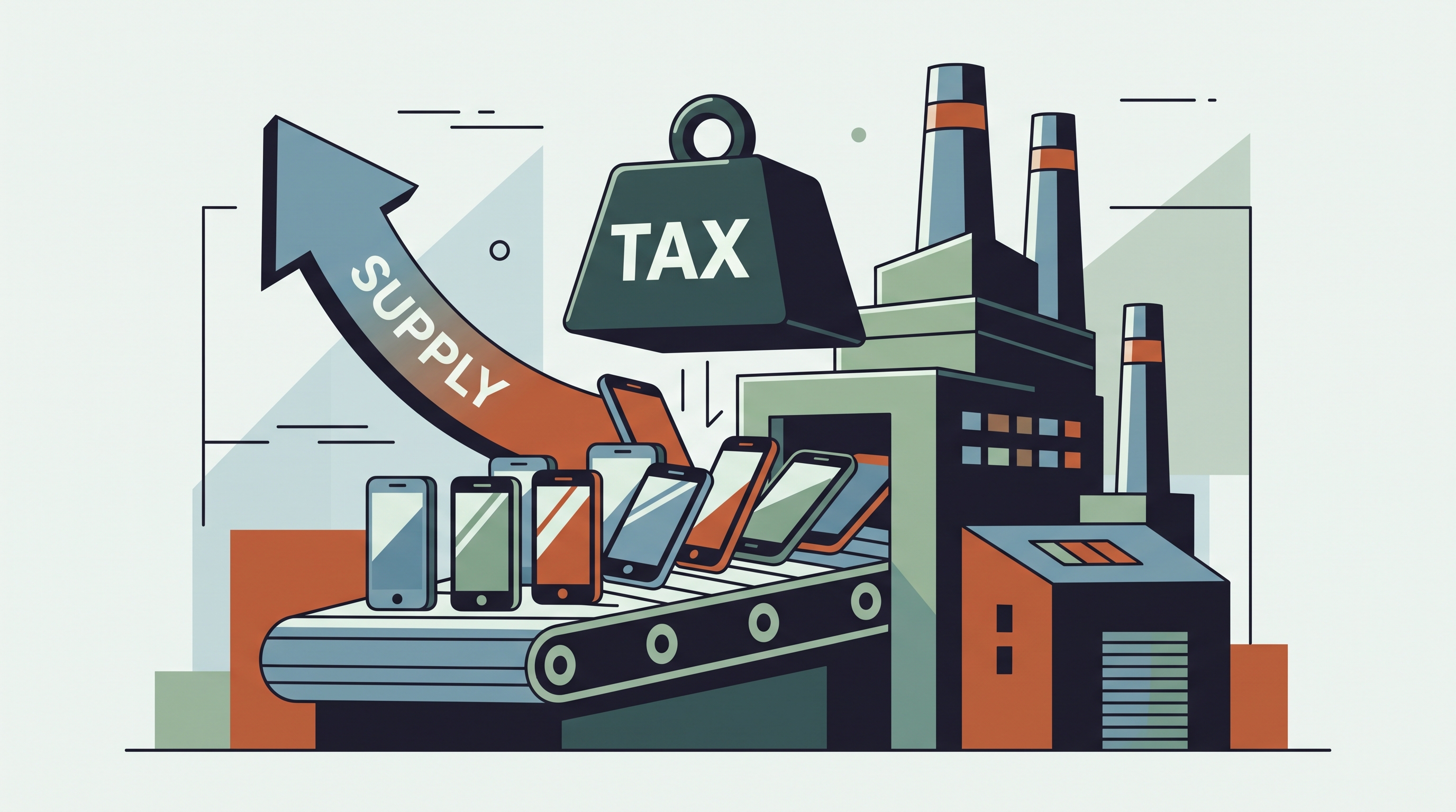
| A per-loaf tax is imposed | Cost per loaf rises | Shifts left |
| A production subsidy is introduced | Effective cost falls | Shifts right |
| Several bakeries exit the market | Fewer sellers remain | Shifts left |
| Producers expect a higher future price | They may hold inventory now | Current supply may shift left |
Worked example. A bakery’s oven becomes 25% more energy-efficient. At a price of $3, it can now profitably produce 150 loaves instead of 120; at every other price, its feasible or profitable quantity is also greater. Because the change affects the quantities offered across the entire schedule, supply shifts right. The price of bread itself did not cause this shift—the technology did.
Misconception check: supply is not inventory
Named misconception — “Supply means the stock sitting on shelves.” Inventory is a quantity of goods already produced. Supply is a planned relationship between possible prices and quantities producers are willing and able to sell. A warehouse full of bread does not automatically mean the supply curve has shifted right; the reason for the inventory change matters.
Another common error is reversing the roles of price and quantity. A higher market price causes an increase in quantity supplied, while lower input costs, improved technology, or more sellers cause an increase in supply. Keep the diagnostic question precise: Did the product’s own price change, or did a nonprice determinant change?
AP skills and reasoning processes
Supply questions commonly assess Skill Category 1: Principles and Models, especially 1.A Define economic concepts, principles, or models and 1.B Explain economic concepts, principles, or models. You must distinguish supply from quantity supplied and connect a determinant—such as an input price or tax—to the correct curve movement.
They also use Skill Category 2: Interpretation, including 2.A Identify economic concepts, principles, or models and 2.B Describe economic concepts, principles, or models, when you read a schedule or graph. Skill Category 3: Manipulation, particularly 3.A Determine the effect of an economic change using quantitative analysis, applies when you add firms’ quantities or interpret numerical schedules. Skill Category 4: Graphing and Visuals, especially 4.A Draw a correctly labeled graph or visual, applies when you label price, quantity, the supply curve, and a directional shift accurately.
Retrieval check
A new tax raises the cost of producing each smartphone. Does the supply curve shift, or does the economy move along the existing curve? Answer: The supply curve shifts left because a nonprice determinant—production cost—changed. A movement along the curve would require a change in the smartphone’s own price.
1.6 Market Equilibrium, Disequilibrium, and Changes in Equilibrium
Key concepts: Market equilibrium · Disequilibrium · Surpluses and shortages · Changes in equilibrium · Shifts in supply and demand · Equilibrium price and quantity · Money market equilibrium · Demand for money · Nominal interest rate · Loanable funds market
A market is in equilibrium when the price makes the quantity buyers want equal to the quantity sellers offer. At that point, neither side has a reason created by the market itself to change its behavior: the market “clears.”
1.6 Market Equilibrium, Disequilibrium, and Changes in Equilibrium
A market is in equilibrium when the price makes the quantity buyers want equal to the quantity sellers offer. At that point, neither side has a reason created by the market itself to change its behavior: the market “clears.”
Equilibrium: $Q_d = Q_s$ at the equilibrium price and equilibrium quantity.
Finding equilibrium in a product market
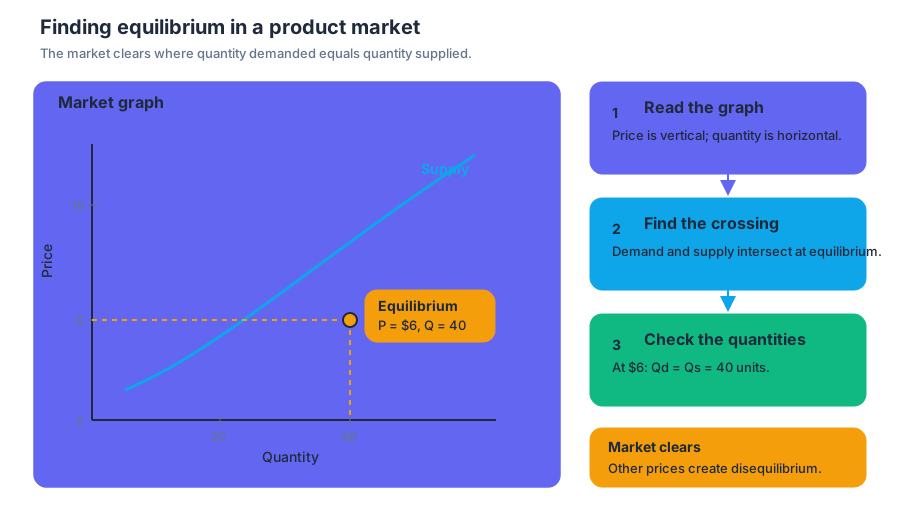
On a standard graph, price is on the vertical axis and quantity is on the horizontal axis. The intersection of demand and supply identifies equilibrium, as required by MKT-2.E: Define market equilibrium, using graphs and MKT-2.E.1: Equilibrium is reached when the price makes quantities demanded and supplied equal.
Suppose a neighborhood market has the following quantities:
| Price | Quantity demanded | Quantity supplied |
|---|---|---|
| $10$ | $20$ | $60$ |
| $6$ | $40$ | $40$ |
| $2$ | $70$ | $20$ |
At a price of $6$, $Q_d = Q_s = 40$, so the equilibrium price is $6$ and the equilibrium quantity is $40$ units. The prices of $10$ and $2$ do not clear the market.
Disequilibrium: surpluses and shortages
Disequilibrium occurs whenever $Q_d \neq Q_s$. A surplus occurs when quantity supplied exceeds quantity demanded:
$$ \text{Surplus} = Q_s - Q_d \quad \text{when } Q_s > Q_d. $$
A shortage occurs when quantity demanded exceeds quantity supplied:
$$ \text{Shortage} = Q_d - Q_s \quad \text{when } Q_d > Q_s. $$
In the example, a price of $10$ creates a surplus of $60 - 20 = 40$ units. Sellers cannot sell everything they planned to sell, so they have an incentive to lower the price. At a price of $2$, the shortage is $70 - 20 = 50$ units; frustrated buyers compete for too few units, giving sellers an incentive to raise the price.
MKT-2.F.1: Whenever markets experience imbalances—creating disequilibrium prices, surpluses, and shortages—market forces drive prices toward equilibrium.
Misconception check — “A surplus means consumers want more.” No. A surplus means sellers offer more than buyers want at the current price. A shortage means buyers want more than sellers offer at the current price. The comparison is always $Q_d$ versus $Q_s$, not total demand versus total supply.
Changes in equilibrium: shift first, intersection second
A change in a determinant of demand or supply shifts an entire curve. The market then moves to a new intersection, producing a new equilibrium price and quantity. This is MKT-2.G: Explain (using graphs as appropriate) how changes in demand and supply affect equilibrium price and equilibrium quantity, supported by MKT-2.G.1: Changes in the determinants of supply and/or demand result in a new equilibrium price and quantity.
Use the graph in two stages:
- Identify which curve shifts and in which direction.
- Read the new price and quantity from the new intersection.
For example, an increase in demand shifts demand right. Equilibrium price rises and equilibrium quantity rises. A decrease in supply shifts supply left. Equilibrium price rises, but equilibrium quantity falls.
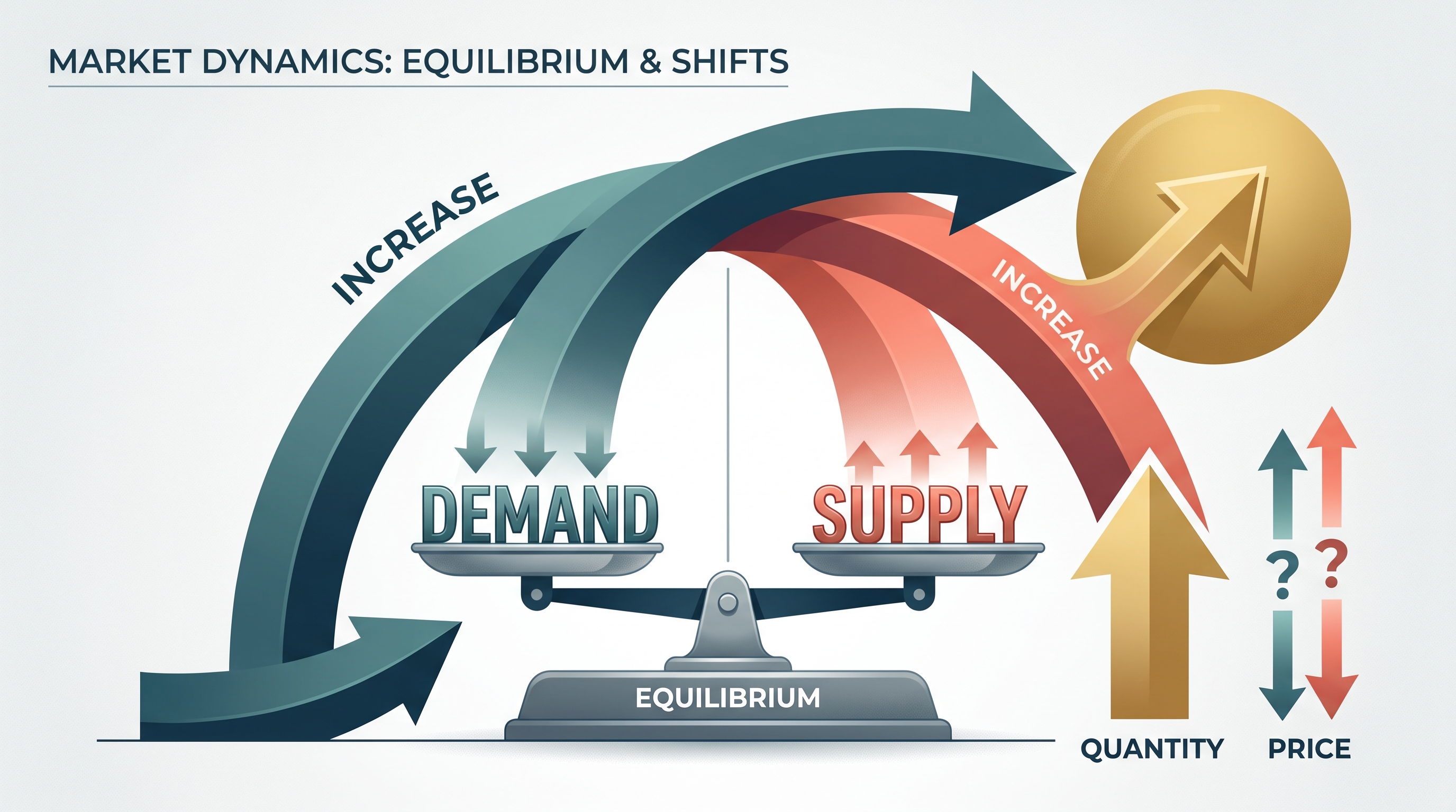
When both curves shift, one result may be determinate while the other is not. An increase in demand and a decrease in supply both raise equilibrium price, but their effects on equilibrium quantity conflict: increased demand pushes quantity up, while decreased supply pushes it down. Therefore, the change in equilibrium quantity is indeterminate without additional information.
An increase in demand and an increase in supply create the opposite problem for price: demand pushes price up, while supply pushes price down. Thus, the change in equilibrium price is indeterminate, although equilibrium quantity increases.
Exam trap: Do not choose an answer that claims both equilibrium variables always move in the same direction. When shifts exert opposing effects, label the result indeterminate.
The same logic in the money market
The money market determines the equilibrium nominal interest rate, the interest rate measured before adjusting for inflation. Its vertical axis measures the nominal interest rate, while its horizontal axis measures the quantity of money.
The demand for money slopes downward because the nominal interest rate is the opportunity cost of holding money rather than an interest-earning financial asset. When the nominal interest rate rises, people want to hold less money; when it falls, they want to hold more. This inverse relationship is MKT-3.A.1: The demand for money shows the inverse relationship between the nominal interest rate and the quantity of money people want to hold.
Factors affecting the value or attractiveness of other financial assets can shift money demand. For instance, if bonds become more attractive, people may reduce the money balances they want to hold, shifting money demand left. The money supply is shown as independent of the nominal interest rate in the basic model, so it is vertical.
Loanable funds: real interest-rate adjustment
The loanable funds market applies the same equilibrium principle to saving and borrowing. MKT-4.D.1 states that disequilibrium real interest rates create surpluses and shortages in this market, while market forces drive the real interest rate toward equilibrium. A real interest rate is approximately:
$$ r \approx i - \pi^e $$
where $i$ is the nominal interest rate and $\pi^e$ is expected inflation.
If the real interest rate is above equilibrium, the quantity of funds supplied exceeds the quantity demanded—a surplus of loanable funds. Lenders compete for borrowers, pushing the real interest rate downward. If it is below equilibrium, a shortage occurs, and competition among borrowers pushes the rate upward.
Skill focus: This topic develops Skill 1.A: Define economic principles and models, Skill 1.B: Explain economic principles and models, Skill 2.B: Interpret economic models, Skill 3.A: Determine outcomes of economic situations, Skill 3.B: Calculate values using economic relationships, and Skill 4.A: Draw graphs and visual representations of economic models. On an exam, earn graphing credit by labeling axes, curves, equilibrium points, and directional shifts; earn explanation credit by completing the causal chain from shift, to disequilibrium, to price or interest-rate adjustment, to the new equilibrium.
Retrieval check
A market begins at equilibrium. Demand increases while supply increases. What happens to equilibrium quantity, and what happens to equilibrium price?
Answer: Equilibrium quantity increases because both shifts raise quantity. Equilibrium price is indeterminate because the demand shift raises price while the supply shift lowers it.
2.1 The Circular Flow and GDP
Key concepts: Circular flow model · Households and businesses · Flow of inputs and outputs · Flow of money · GDP as total income and expenditure · GDP as final output · Expenditure approach to measuring GDP · Income approach to measuring GDP · Value-added approach to measuring GDP · GDP components
Every purchase is simultaneously someone else’s income: when a household buys a $5 sandwich, the household records consumption spending, while the bakery records $5 of revenue.
2.1 The Circular Flow and GDP
Every purchase is simultaneously someone else’s income: when a household buys a $5 sandwich, the household records consumption spending, while the bakery records $5 of revenue. The circular flow model turns this simple exchange into a picture of how an entire economy connects.
Enduring Understanding MEA-1: An economy’s performance can be measured by different indicators, including gross domestic product ($GDP$), the inflation rate, and the unemployment rate.
Learning Objective MEA-1.A: Define, using the circular flow diagram as appropriate, how GDP is measured and its components; calculate nominal GDP.
The two main participants
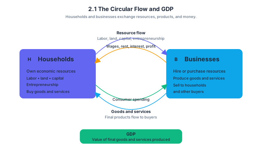
The circular flow model represents two broad groups:
- Households own the economic resources—labor, land, capital, and entrepreneurship—and sell the use of those resources to businesses.
- Businesses hire or purchase those resources to produce goods and services, which they sell to households and other buyers.
This simplified model does not mean that households and businesses are the only real participants in an economy. Rather, it isolates the basic relationship between resource owners and producers so that the movement of goods, services, resources, and money is visible.
Real flows and money flows
The model contains two connected circuits. The real flow consists of physical or productive activity: households provide inputs, businesses transform those inputs into outputs, and households receive goods and services. The money flow moves in the opposite direction: businesses pay households for inputs, and households pay businesses for final goods and services.
A useful way to read the model is to ask two questions at every arrow:
- What is moving? Resources, goods, services, or money?
- Who receives payment or income?
For example, a student works at a grocery store. The student supplies labor, an input, to the business and receives wages. The store uses labor, equipment, buildings, and inventory to produce retail services. When a household buys groceries, its spending becomes the store’s revenue, which helps pay workers, suppliers, lenders, and owners.
Key insight: One person’s expenditure is another person’s income.
GDP: final output, income, and expenditure
Gross domestic product ($GDP$) is the market value of all final goods and services produced within a country during a given period. “Final” means the product is ready for its ultimate user; intermediate goods are excluded so that the same production is not counted repeatedly.
GDP can therefore be understood in three equivalent ways:
| Approach | What it adds up | Central question |
|---|---|---|
| Expenditures approach | Spending on final goods and services | Who bought the final output? |
| Income approach | Income earned from producing output | Who received income from production? |
| Value-added approach | Value added at every production stage | How much new value did each producer create? |
The equality works because the economy’s final output generates revenue; that revenue becomes income to the people and firms involved in production. The value-added approach reaches the same total without double-counting intermediate transactions.
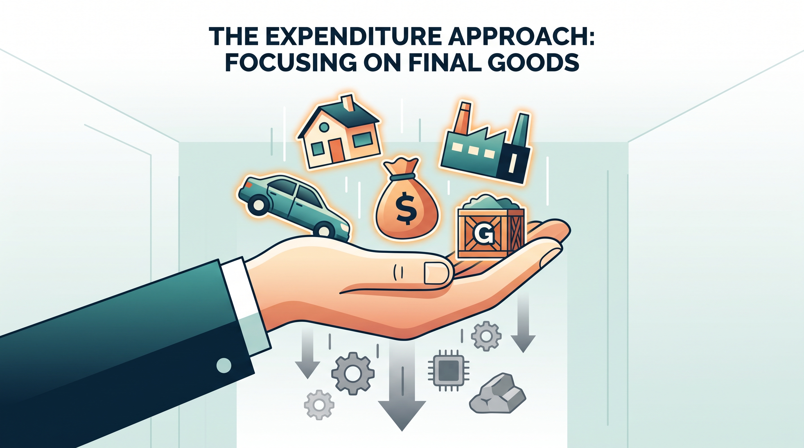
The expenditures approach
The standard expenditure identity is
$$GDP = C + I + G + NX$$
where:
- $C$ = household consumption spending;
- $I$ = business investment spending, including purchases of capital goods and construction of new structures;
- $G$ = government purchases of newly produced goods and services;
- $NX$ = net exports, calculated as exports minus imports: $NX = X - M$.
Suppose an economy records $C = $700$ billion, $I = $180$ billion, $G = $220$ billion, exports of $$90$ billion, and imports of $$120$ billion. Then
$$NX = 90 - 120 = -$30\text{ billion}$$
and
$$GDP = 700 + 180 + 220 - 30 = $1{,}070\text{ billion}.$$
Imports are subtracted because they may already be included in $C$, $I$, or $G$, but they were produced outside the country. Exports are added because they are domestic production purchased by foreigners.
Value added: avoiding double counting
Imagine that a farmer sells wheat for $$2$ to a mill, the mill sells flour for $$5$ to a baker, and the baker sells bread for $$9$ to a household. Adding every sale gives $$16$, but that exaggerates production because the wheat and flour are embedded in the final bread.
The value-added approach counts only the new value created at each stage:
$$$2 + ($5-$2) + ($9-$5) = $9.$$
The result equals the value of the final bread, which is the amount included in GDP.
Misconception check
Misconception: “GDP is every transaction in the economy.” It is not. GDP measures final domestic production during the period. A used bicycle sold this year is generally excluded because it was produced earlier, while a newly produced bicycle is included.
Skills in action
This topic primarily develops Skill 1.A: Define economic principles and models, Skill 1.B: Explain economic principles and models, Skill 2.A: Identify economic concepts, principles, and models, Skill 2.C: Explain given economic outcomes, Skill 3.B: Calculate economic outcomes, and Skill 4.A: Draw graphs and visual representations. On an exam, these skills appear when you interpret arrows in a circular-flow diagram, explain why income equals expenditure, calculate GDP, or label relationships between households and businesses.
Retrieval check
A household purchases a newly produced laptop for $$1{,}200$. The laptop contains imported components worth $$300$. The purchase is household consumption, so it initially enters $C$ at $$1{,}200$; the imported portion is removed through $M$. Why must the expenditure approach exclude intermediate goods, and which GDP approach makes that logic most explicit?
2.2 Limitations of GDP
Key concepts: quantitative analysis in economics · interpretation and application of quantitative analysis · economic indicators · explaining indicators
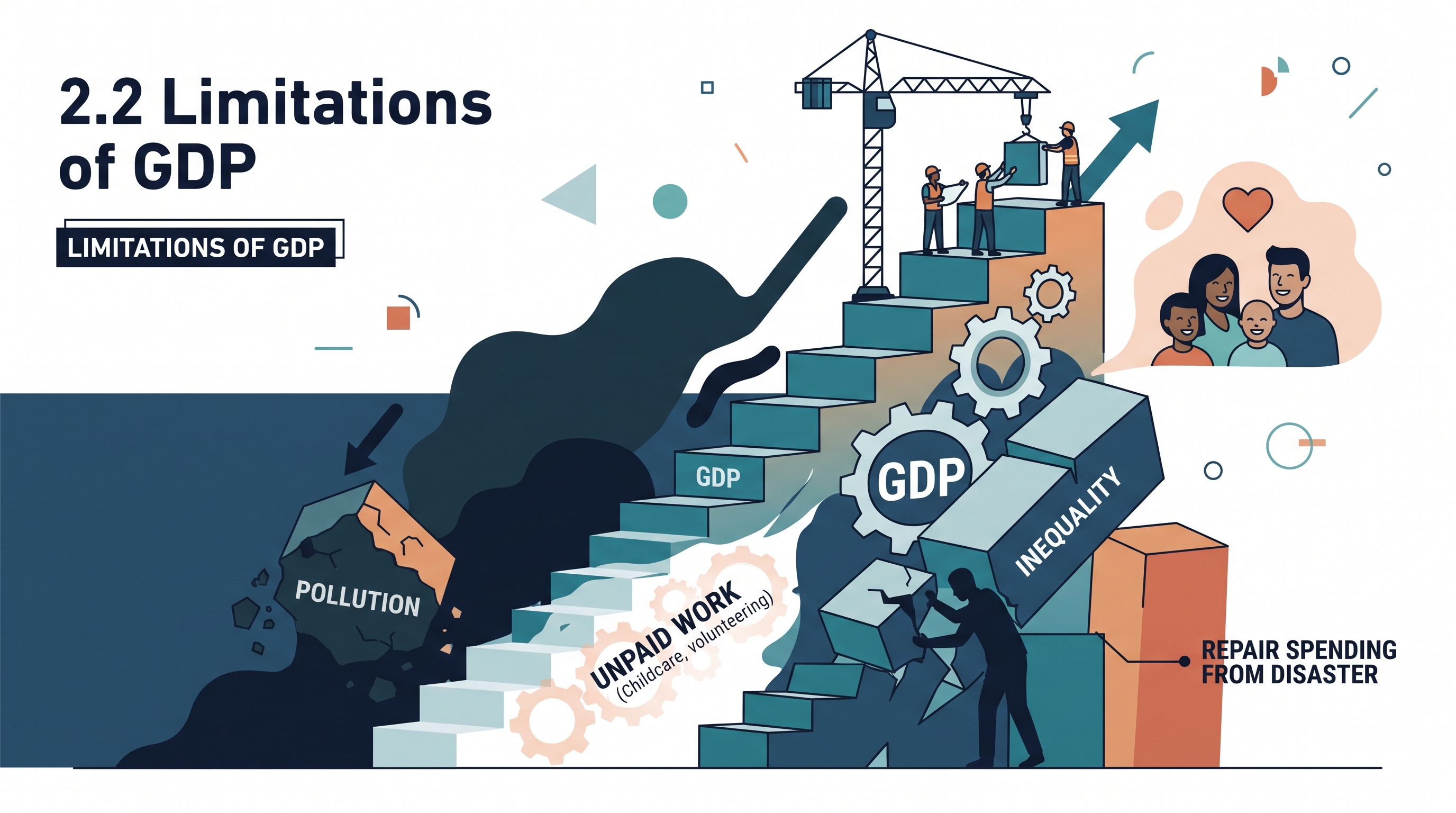
GDP can rise while many people’s lives fail to improve, because production is not the same thing as well-being. Using the GDP measure of market production established in 2.1, the key question is: What does this indicator measure accurately, and what does it leave out?
2.2 Limitations of GDP
GDP can rise while many people’s lives fail to improve, because production is not the same thing as well-being. Using the GDP measure of market production established in 2.1, the key question is: What does this indicator measure accurately, and what does it leave out?
Learning Objective MEA-1.B: Explain the limitations of using GDP as a measure of economic well-being.
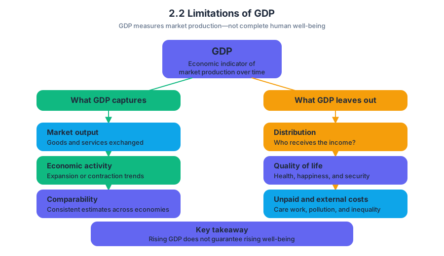
GDP is valuable because it provides a consistent estimate of market production over a period of time. It helps economists compare economies, identify changes in economic activity, and evaluate whether output is expanding or contracting. But GDP is an economic indicator, meaning a numerical measure used to describe an aspect of economic performance—not a complete scorecard for human welfare.
What GDP captures—and what it misses
The most important distinction is between production and well-being. GDP counts the market value of final goods and services, but the same amount of production can produce very different outcomes for health, safety, equality, leisure, and environmental quality.
| GDP may record… | But GDP does not fully reveal… |
|---|---|
| More medical services purchased | Whether people are healthier |
| More spending after storm damage | The loss of homes, safety, or natural resources |
| More factory output | Pollution and damage caused by production |
| Paid childcare services | The value of unpaid care provided at home |
| Higher total output | How income and output are distributed |
| More hours worked | Whether people have less leisure or quality of life |
Several limitations follow from this distinction:
- Nonmarket activity: Unpaid household work, volunteer work, and care provided within families may create real value without involving a market transaction.
- Income distribution: GDP is a total. It does not show whether additional income is broadly shared or concentrated among a small group.
- Environmental quality: Production that creates pollution may increase GDP even when it reduces health or damages ecosystems.
- Quality of life: GDP does not directly measure leisure, personal safety, political freedom, social connection, or access to clean surroundings.
- Quality and composition of output: Two economies with equal GDP may produce different combinations of goods and services, with different consequences for residents.
- Underground or unreported activity: Economic transactions that are hidden from official measurement may not be fully included.
These limitations do not make GDP useless. They establish a boundary around the claim an economist may make. A rising GDP supports the statement that measured market production increased; it does not, by itself, prove that every household became better off.
Worked interpretation: the same GDP, different lives
Suppose Country A and Country B each report GDP of $500$ billion. Country A has clean air, widely distributed income, extensive unpaid family care, and shorter workweeks. Country B has severe pollution, unequal income, and long workweeks, while many essential household services are performed without pay. GDP alone cannot determine which country has greater economic well-being.
A careful explanation proceeds in three steps:
- Identify what the indicator measures: both countries report the same measured market production.
- State the valid comparison: their GDP totals are equal, so GDP does not distinguish their market output.
- Identify omitted dimensions: distribution, environmental quality, unpaid activity, and leisure may differ substantially.
This is quantitative analysis in economics: not merely calculating or reading a number, but interpreting what the number means and applying it to a specific context. A response that says “GDP is $500$ billion” performs measurement; a response that explains what that figure can and cannot establish performs economic reasoning.
A useful mental model
Imagine GDP as a dashboard gauge labeled market production. The gauge is useful, but it has no sensors for every variable that matters to human welfare. A responsible analyst reads the gauge precisely, then asks which important conditions remain outside its measurement.
Common misconception: “Higher GDP always means higher well-being”
Correction: Higher GDP can indicate greater capacity to purchase goods and services, but it is not conclusive evidence of higher overall well-being. The direction of GDP and the direction of welfare may differ when pollution increases, income becomes more unequal, unpaid work replaces paid work, or destructive events generate repair spending.
Skill connections: Topic 2.2 most directly develops Skill Category 2: Interpretation, especially 2.A: Define economic indicators, 2.B: Explain economic indicators, and 2.C: Interpret quantitative data. It also uses Skill Category 1: Principles and Models—1.A: Define economic principles and models and 1.B: Explain economic principles and models—when distinguishing an indicator’s measured variable from the broader concept of well-being. In an exam response, the strongest reasoning identifies the indicator, states its measurable meaning, applies the limitation to the context, and avoids claiming more than the data support.
Retrieval check: If GDP increases after a major hurricane because construction and repair spending rise, can an economist conclude that residents’ well-being increased? Answer: No. Measured production may have increased, but GDP does not subtract the destruction, lost safety, disrupted lives, or environmental damage caused by the hurricane.
2.3 Unemployment
A person is unemployed only when they do not have a job, are available to work, and are actively looking for work. That final condition is crucial: unemployment statistics measure participation in the labor market, not simply whether someone currently receives a paycheck.
2.3 Unemployment
A person is unemployed only when they do not have a job, are available to work, and are actively looking for work. That final condition is crucial: unemployment statistics measure participation in the labor market, not simply whether someone currently receives a paycheck.
The labor-market categories
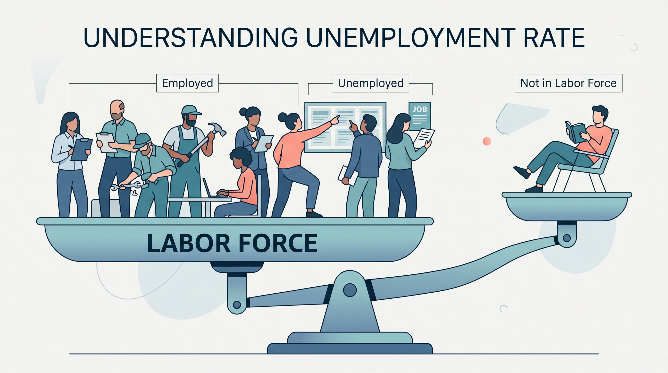
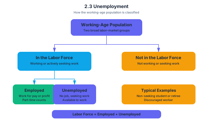
The working-age population is divided into people in the labor force and people not in the labor force. The labor force contains both employed people and unemployed people:
$$ \text{Labor Force}=\text{Employed}+\text{Unemployed} $$
A person is employed if they performed work for pay or profit during the measurement period, even if the work was part-time. A person is unemployed if they have no job but are actively seeking and available for work. A student who is not looking for a job, a retired person, and a person who has stopped searching because jobs seem unavailable are classified as not in the labor force, not unemployed.
Measuring unemployment
The unemployment rate is the percentage of the labor force that is unemployed:
$$ \text{Unemployment Rate}
\frac{\text{Number of Unemployed}}{\text{Labor Force}} \times 100 $$
The denominator is not the entire working-age population. This distinction makes the rate an indicator of conditions among people participating in the labor market.
The labor-force participation rate measures the percentage of the working-age population that is in the labor force:
$$ \text{Labor-Force Participation Rate}
\frac{\text{Labor Force}}{\text{Working-Age Population}} \times 100 $$
The two rates answer different questions: the unemployment rate asks how many labor-force participants lack jobs, while the participation rate asks how many working-age people are working or looking for work.
Worked example: calculating both rates
Suppose a town has a working-age population of $1{,}000$. Of these people, $620$ are employed, $40$ are unemployed and actively seeking work, and $340$ are not in the labor force.
First calculate the labor force:
$$ \text{Labor Force}=620+40=660 $$
Then calculate the unemployment rate:
$$ \frac{40}{660}\times 100\approx 6.1% $$
Finally calculate the labor-force participation rate:
$$ \frac{660}{1{,}000}\times 100=66% $$
Interpretation: $6.1%$ of labor-force participants are unemployed, while $66%$ of the working-age population is participating in the labor market.
Three types of unemployment
Frictional unemployment is short-term unemployment caused by workers moving between jobs or entering the labor market. A recent graduate searching for a first job is frictionally unemployed.
Structural unemployment occurs when workers’ skills, locations, or training do not match the jobs available. A factory worker whose industry adopts new technology may need retraining before finding suitable employment.
Cyclical unemployment results from downturns in the business cycle. When aggregate demand falls during a recession, firms reduce production and may lay off workers. Cyclical unemployment therefore rises during recessions and falls during expansions.
The natural rate of unemployment is the unemployment rate that exists when the economy has no cyclical unemployment. It includes frictional and structural unemployment:
$$ \text{Natural Rate}
\text{Frictional Rate} + \text{Structural Rate} $$
Actual unemployment can be expressed as:
$$ \text{Actual Unemployment}
\text{Natural Unemployment} + \text{Cyclical Unemployment} $$
Misconception check: “Everyone without a job is unemployed”
This is the most common classification error. A person who wants a job but has stopped searching is not counted as unemployed under the standard measure because they are not actively seeking work. If that person begins searching, the labor force increases and the unemployment rate may rise—even if no employed person loses a job.
Another error is assuming that a higher unemployment rate always means fewer people work. If discouraged workers begin searching, the number unemployed can increase while employment remains unchanged. Always inspect the labor force and participation rate before interpreting the percentage.
AP skills and reasoning processes
This topic is assessed through Skill Category 1: Principles and Models, especially 1.A Define economic principles and models and 1.B Explain economic outcomes using economic concepts, principles, and models; Skill Category 2: Interpretation, especially 2.A Define economic variables, 2.B Explain economic variables, and 2.C Interpret economic data; Skill Category 3: Manipulation, especially 3.B Calculate numerical outcomes; and Skill Category 4: Graphing and Visuals, especially 4.B Explain relationships within graphs and visual representations. On an exam, these skills appear as labor-force calculations, classification decisions, data interpretation, and explanations connecting cyclical unemployment to the business cycle.
Retrieval check: A population contains $800$ employed people, $100$ unemployed people actively seeking work, and $300$ people outside the labor force. What is the unemployment rate?
Answer: The labor force is $800+100=900$. Therefore,
$$ \text{Unemployment Rate}
\frac{100}{900}\times 100 \approx 11.1% $$
The $300$ people outside the labor force do not belong in the denominator.
2.4 Price Indices and Inflation
Key concepts: Price indices · Consumer Price Index (CPI) · GDP deflator · Inflation, deflation, and disinflation · Inflation rate · Nominal and real variables · Shortcomings of the CPI · Costs of unexpected inflation · Real wages · Comparing nominal variables over time
A price index turns a changing collection of prices into one number: it measures the general price level in a given period relative to the prices in a chosen base year.
2.4 Price Indices and Inflation
A price index turns a changing collection of prices into one number: it measures the general price level in a given period relative to the prices in a chosen base year. If the index rises from $100$ to $105$, the economy’s measured price level has increased by $5%$ relative to the base year—not necessarily that every individual price rose by exactly $5%$.
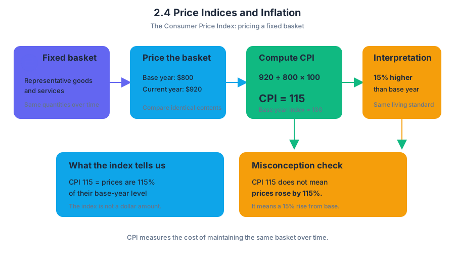
Essential idea — MEA-1.F.2: The CPI measures the cost of a fixed basket of goods and services in a given year relative to the cost of that basket in the base year.
The topic’s enduring understanding, MEA-1, treats the inflation rate as one indicator of an economy’s performance alongside GDP and unemployment. The required learning objective MEA-1.F asks you to define and calculate price measures, use them to compare nominal values across time, and determine changes in real variables; MEA-1.G adds the limitations of the CPI as a measure of true inflation.
The Consumer Price Index: pricing a fixed basket
The Consumer Price Index (CPI) measures how the cost of a fixed market basket of consumer goods and services changes over time. In practical terms, it estimates how much income a household would need in a later year to maintain the same standard of living it had in the base year.
The calculation is:
$$ \text{CPI}=\frac{\text{Cost of market basket in current year}}{\text{Cost of market basket in base year}}\times 100 $$
Suppose a representative basket costs $800$ in the base year and $920$ today. Then:
$$ \text{CPI}=\frac{920}{800}\times 100=115 $$
A CPI of $115$ means the basket costs $15%$ more than it did in the base year. The number $115$ is an index value, not a dollar amount and not itself the inflation rate for the current year.
Misconception check: A CPI of $115$ does not mean that prices rose by $115%$. It means prices are $115%$ of their base-year level, or $15%$ above it.
Inflation, deflation, and disinflation
Inflation is a sustained increase in the general price level. Deflation is a decrease in the general price level, while disinflation is a decline in the inflation rate—the price level is still rising, but more slowly.
| Situation | Price-level movement | Inflation-rate movement |
|---|---|---|
| Inflation | Increases | Positive |
| Deflation | Decreases | Negative |
| Disinflation | Still increases | Positive but falling |
The inflation rate is the percentage change in a price index:
$$ \text{Inflation rate}= \frac{\text{Current price index}-\text{Previous price index}} {\text{Previous price index}}\times 100 $$
If the CPI rises from $120$ to $126$:
$$ \text{Inflation rate}=\frac{126-120}{120}\times100=5% $$
If the CPI rises from $126$ to $128$, inflation is:
$$ \frac{128-126}{126}\times100\approx1.6% $$
Prices are still increasing, so this is not deflation. Because inflation fell from $5%$ to approximately $1.6%$, it is disinflation.
CPI and the GDP deflator
The GDP deflator is another price index. It compares the value of all final goods and services produced domestically at current prices with their value at base-year prices:
$$ \text{GDP deflator}= \frac{\text{Nominal GDP}}{\text{Real GDP}}\times100 $$
For example, if nominal GDP is $525$ billion and real GDP is $500$ billion:
$$ \text{GDP deflator}=\frac{525}{500}\times100=105 $$
A GDP deflator of $105$ means that the prices of domestically produced final output are, on average, $5%$ higher than in the base year. The CPI and GDP deflator are both price indices, but the CPI uses a fixed consumer basket, whereas the GDP deflator covers domestically produced final output.
Scope note — MEA-1.F.2: Calculating the producer price index, or PPI, is beyond the scope of the AP Macroeconomics course and exam.
Nominal and real variables
A nominal variable is measured using the prices that exist at the time of measurement—for example, nominal wages or nominal GDP. A real variable has been adjusted for changes in the price level; MEA-1.F.4 defines real variables as nominal variables deflated by the price level.
Price indices allow meaningful comparisons across years. If a worker’s nominal wage rises by $10%$ while inflation is $15%$, purchasing power falls: the worker can buy less than before. Using the approximation:
$$ \text{Real wage change}\approx\text{Nominal wage change}-\text{Inflation rate} $$
Therefore:
$$ 10%-15%=-5% $$
The worker’s real wage decreases by approximately $5%$. A larger paycheck does not guarantee a higher standard of living when prices rise faster than wages.
Limits of the CPI
Under MEA-1.G, the CPI is useful but imperfect. Because it follows a fixed basket, it may overstate the true rise in the cost of maintaining a standard of living: consumers can substitute toward relatively cheaper goods, new products may improve purchasing options, and measured prices may not fully capture quality changes.
Unexpected inflation also redistributes wealth arbitrarily. For instance, a borrower who repays a fixed-rate loan with dollars that have lost purchasing power gains relative to the lender, because the lender receives less real value than expected.
Skill in action: 2.C Interpretation
AP Skill 2.C — Interpretation means interpreting a specific economic outcome using quantitative data or calculations. On an exam, do not stop after computing $105$ or $5%$: state what the number means economically—whether the price level rose or fell, whether inflation accelerated or slowed, and whether purchasing power increased or decreased.
Retrieval check: A price index falls from $110$ to $104$. Is this inflation, deflation, or disinflation? Calculate the rate:
$$ \frac{104-110}{110}\times100\approx-5.5% $$
Because the index itself fell and the inflation rate is negative, the result is deflation, not disinflation.
2.5 Costs of Inflation
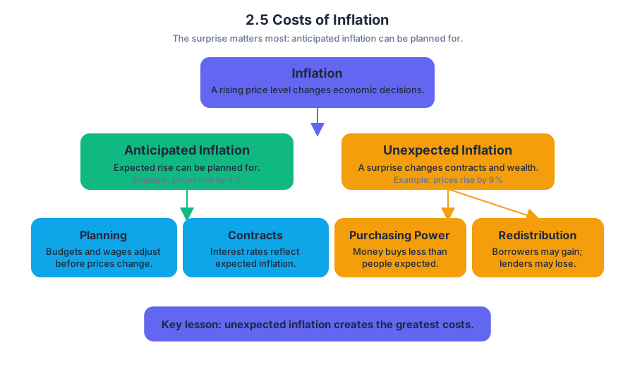
Inflation creates costs because a rising price level makes economic decisions harder, changes the value of contracts, and can redistribute purchasing power between people. The damage is greatest when inflation is unexpected rather than merely positive.
2.5 Costs of Inflation
Inflation creates costs because a rising price level makes economic decisions harder, changes the value of contracts, and can redistribute purchasing power between people. The damage is greatest when inflation is unexpected rather than merely positive.
LO 2.5.A — Explain the costs of inflation.
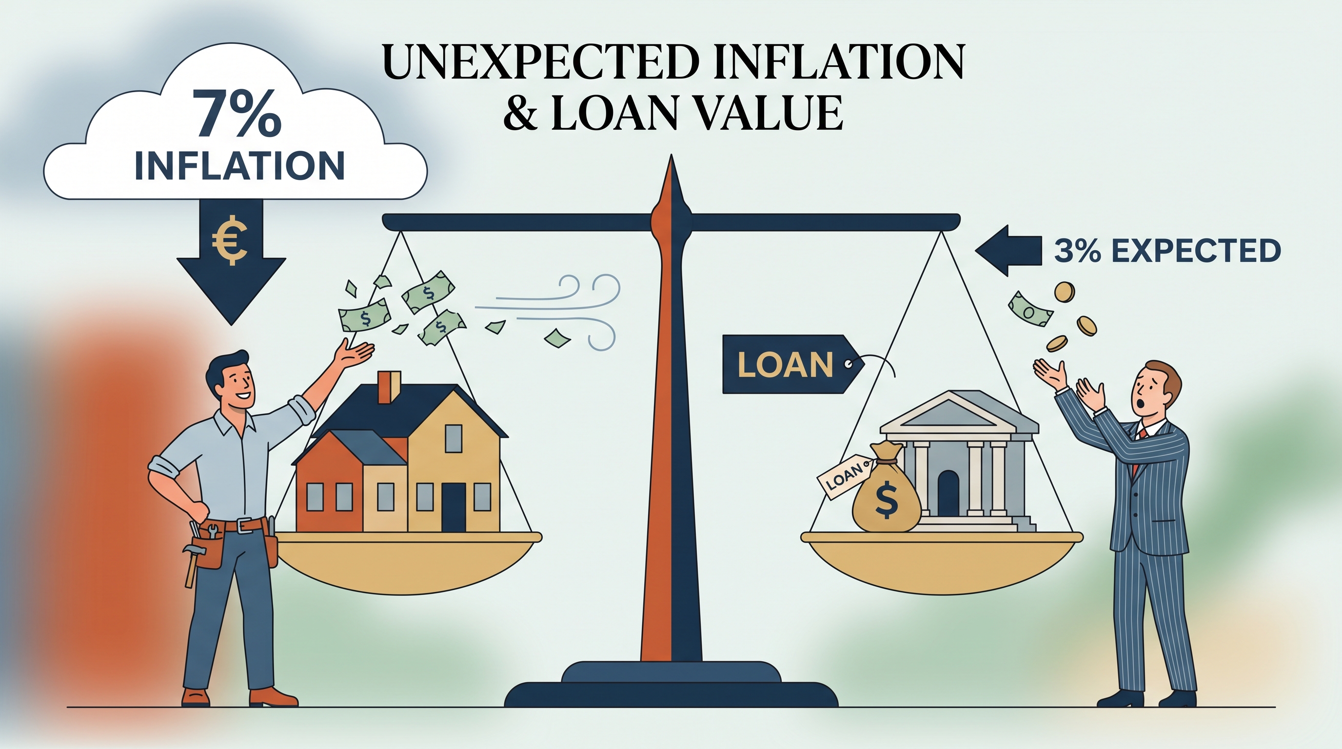
The central distinction is anticipated inflation versus unexpected inflation. If households and firms correctly expect prices to rise by $4%$, they can adjust wages, contracts, interest rates, and budgets. If prices instead rise by $9%$, the surprise changes who gains and who loses.
The predictable costs of a rising price level
Even anticipated inflation consumes real resources. People and firms must spend time and effort changing prices, recalculating budgets, and managing cash balances. These costs are commonly grouped into three categories.
| Cost | What changes | Concrete example |
|---|---|---|
| Menu costs | Firms must update posted prices, catalogs, labels, and software | A restaurant repeatedly reprints menus as ingredient costs rise |
| Shoe-leather costs | People make more frequent trips or transactions to avoid holding cash that loses purchasing power | A household visits the bank more often or moves money between accounts |
| Unit-of-account costs | Prices become less useful as a measuring stick for comparing values | A business has difficulty judging whether a higher price reflects improved quality or general inflation |
The phrase shoe-leather is a metaphor: frequent trips to manage money wear out shoes. The underlying idea is that inflation makes money balances more expensive to hold because each dollar buys fewer goods and services over time.
Unexpected inflation redistributes purchasing power
Unexpected inflation changes the real value of payments that were fixed in nominal terms. A nominal value is measured in current dollars; the real value is its purchasing power after accounting for the price level. When inflation is higher than expected, borrowers generally gain and lenders generally lose because the borrower repays with dollars that buy less.
Worked example: a fixed-rate loan
Suppose a student borrows $10{,}000$ at a fixed nominal interest rate of $5%$. The repayment due after one year is:
$$ $10{,}000(1.05)=$10{,}500 $$
If the expected inflation rate was $2%$, the approximate expected real interest rate would be:
$$ 5%-2%=3% $$
But if actual inflation unexpectedly reaches $8%$, the approximate actual real interest rate becomes:
$$ 5%-8%=-3% $$
The lender receives $10{,}500$ nominal dollars, but those dollars have less purchasing power than expected. The borrower benefits from repaying a debt whose real burden has fallen. The reverse occurs when inflation is lower than expected: lenders gain and borrowers lose relative to their expectations.
Other distributional and decision-making costs
Unexpected inflation can also redistribute income between workers and employers. If wages are fixed by a contract and prices rise faster than expected, workers’ real wages fall temporarily, while the firm’s labor costs are lower in real terms. If wages adjust immediately but product prices are fixed, the distribution can move in the opposite direction.
Inflation can distort tax outcomes when tax brackets or deductions do not adjust perfectly with prices. A worker whose nominal income rises only because of inflation may move into a higher tax bracket even though the worker’s real purchasing power has barely increased. Inflation can therefore reduce the incentive to save, invest, or work when tax rules and contracts fail to adjust.
Uncertainty is an additional cost. When firms cannot predict future input prices, wages, or borrowing costs, they may postpone investment or make less efficient production decisions. Households also find long-term planning—such as saving for education or retirement—more difficult when the future purchasing power of money is unclear.
Misconception check
Misconception: “Inflation makes everyone poorer by exactly the same amount.”
Inflation does not affect everyone identically. The outcome depends on whether a person’s income, assets, debts, and contracts adjust with the price level. A borrower with a fixed-rate loan may gain from unexpected inflation, while the lender loses; a worker with a cost-of-living adjustment may be protected, while a worker with a fixed nominal wage may lose purchasing power.
Retrieval check
A bank makes a fixed-rate loan expecting inflation of $3%$, but actual inflation is $7%$. Who benefits, and why? Answer: the borrower benefits because the fixed repayment is made with dollars whose purchasing power has fallen more than expected; the lender receives a lower-than-expected real return.
2.6 Real versus Nominal GDP
Key concepts: Nominal GDP · Real GDP · Base-year pricing · Calculating real GDP · Calculating nominal GDP · Price-level changes · Real versus nominal values · GDP price weighting · Fixed quantities · Effects of inflation on GDP comparisons
A country can produce more goods while its GDP rises—or report higher GDP simply because prices increased. Nominal GDP and real GDP separate these two forces by asking two different questions: How much was current production worth at current prices?
2.6 Real versus Nominal GDP
A country can produce more goods while its GDP rises—or report higher GDP simply because prices increased. Nominal GDP and real GDP separate these two forces by asking two different questions: How much was current production worth at current prices? and How much would that production be worth if prices were held constant?
Two ways to value the same output
Nominal GDP is the value of current output using current-year prices. It changes when either production quantities or prices change:
$$\text{Nominal GDP}=\sum(\text{current-year price}\times\text{current-year quantity})$$
Real GDP is the value of current output using prices from a designated base year, the reference year whose prices are held constant:
$$\text{Real GDP}=\sum(\text{base-year price}\times\text{current quantity})$$
The quantities can change from year to year, but the prices used in real GDP remain fixed. That makes real GDP a measure of changes in actual output, rather than a mixture of output changes and price-level changes.
| Measure | Prices used | Quantities used | What a change can reflect |
|---|---|---|---|
| Nominal GDP | Current-year prices | Current-year quantities | Changes in prices, quantities, or both |
| Real GDP | Base-year prices | Current-year quantities | Changes in quantities, or real output |
Middleland: holding prices constant
Suppose Middleland produces food, clothing, and machinery. In the base year, 2021, the table gives these prices and quantities:
| Good | 2021 price | 2021 quantity | 2022 quantity |
|---|---|---|---|
| Food | $50 | $11$ units | $10$ units |
| Clothing | $70 | $4$ units | $5$ units |
| Machinery | $30 | $12$ units | $15$ units |
In the base year, 2021, real GDP equals nominal GDP because both calculations use the same prices:
$$\text{GDP}_{2021}=(11\times 50)+(4\times 70)+(12\times 30)$$
$$\text{GDP}_{2021}=550+280+360=$1{,}190$$
Thus, in 2021:
$$\text{Real GDP}{2021}=\text{Nominal GDP}{2021}=$1{,}190$$
Using the stated Middleland comparison, 2022 real GDP is calculated with 2021 prices:
$$\text{Real GDP}_{2022}=(11\times 50)+(4\times 70)+(12\times 30)=$1{,}190$$
The central operation is the price substitution: use base-year prices while evaluating the relevant output at constant prices. By contrast, 2022 nominal GDP uses 2022 prices and quantities:
$$\text{Nominal GDP}_{2022}=(10\times 50)+(5\times 70)+(15\times 30)$$
$$\text{Nominal GDP}_{2022}=500+350+450=$1{,}300$$
The GDP deflator and price weighting
The GDP deflator is a broad price index for domestically produced final goods and services. It compares nominal GDP with real GDP:
$$\text{GDP deflator}=\left(\frac{\text{Nominal GDP}}{\text{Real GDP}}\right)\times 100$$
For Middleland in 2022:
$$\text{GDP deflator}_{2022}=\left(\frac{1{,}300}{1{,}190}\right)\times 100\approx 109.2$$
A deflator of approximately $109.2$ means the measured price level is about $9.2%$ above the base-year level of $100$. Unlike a simple average of price changes, the GDP deflator is quantity-weighted: goods produced in larger quantities, or goods with greater production value, exert more influence on the overall price measure than goods with smaller weights. A large change in the price of a rarely produced good may matter less than a modest change in the price of a major component of national output.
What changes in GDP actually mean
If nominal GDP rises from $$1{,}190$ to $$1{,}300$ while real GDP is held at $$1{,}190$, the increase in nominal GDP reflects the pricing method rather than an increase in measured real output. Real GDP is designed to prevent price-level fluctuations from masquerading as production growth.
Key distinction: Nominal GDP answers “What was current production worth at today’s prices?” Real GDP answers “What would current production be worth at constant base-year prices?”
Misconception check: “Higher nominal GDP means the economy produced more.”
Not necessarily. A bakery could sell the same number of loaves at higher prices, causing nominal GDP to rise even though output is unchanged. To identify a change in production, economists use real GDP, which removes the price-change component by fixing prices at the base-year level.
Retrieval check
If nominal GDP is $$1{,}300$ and real GDP is $$1{,}190$, calculate the GDP deflator. What does a result above $100$ indicate?
The answer is:
$$\left(\frac{1{,}300}{1{,}190}\right)\times 100\approx 109.2$$
A value above $100$ indicates that the current measured price level is above the base-year price level.
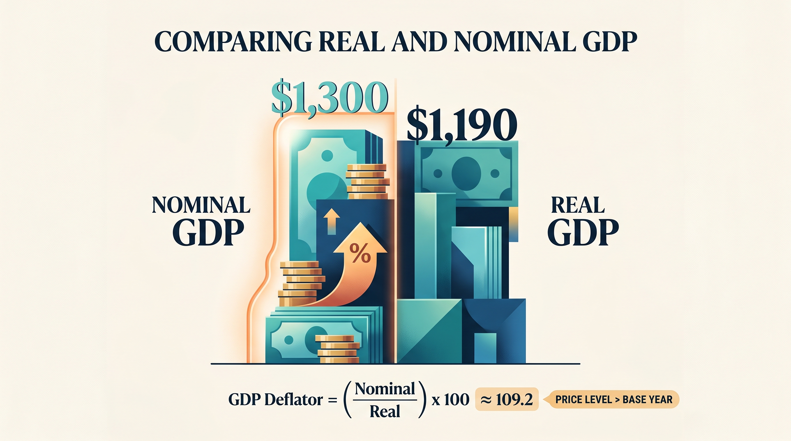
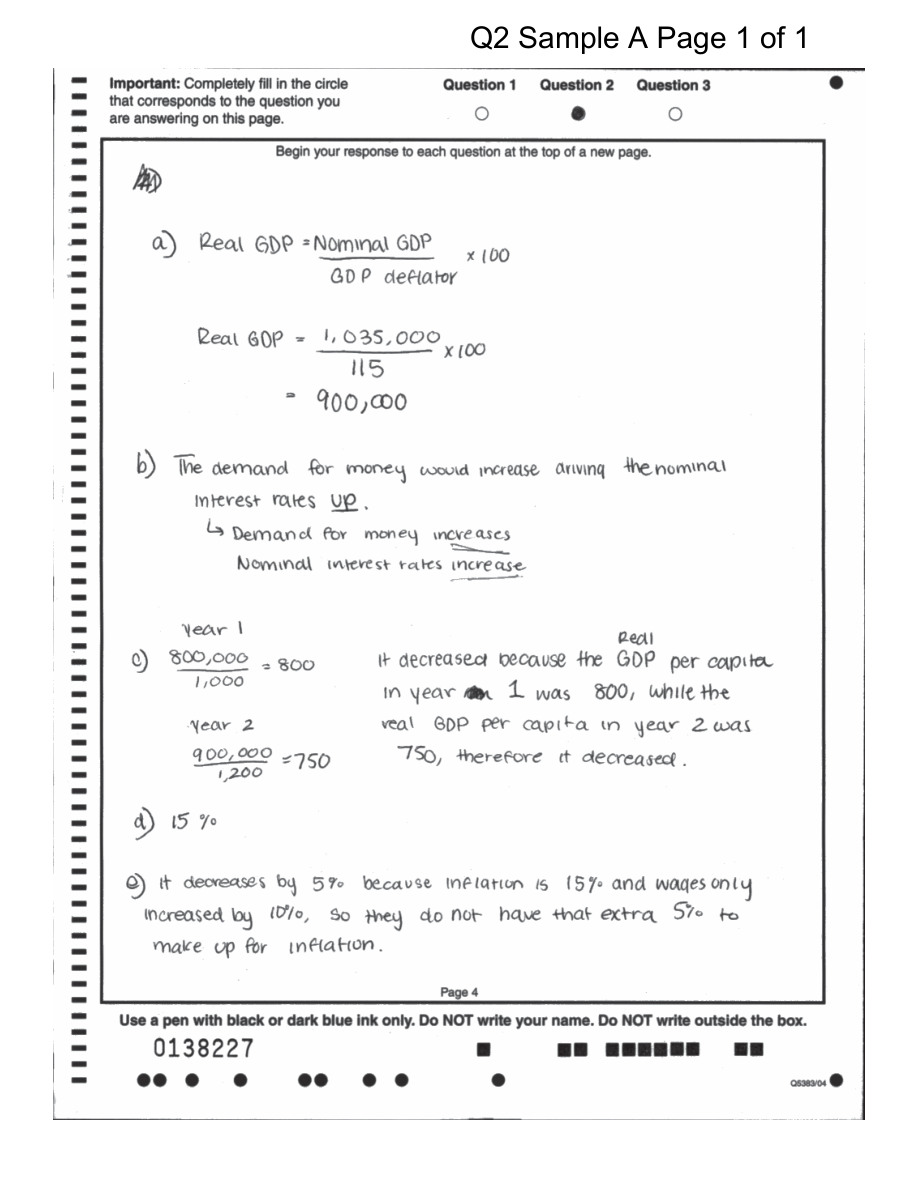
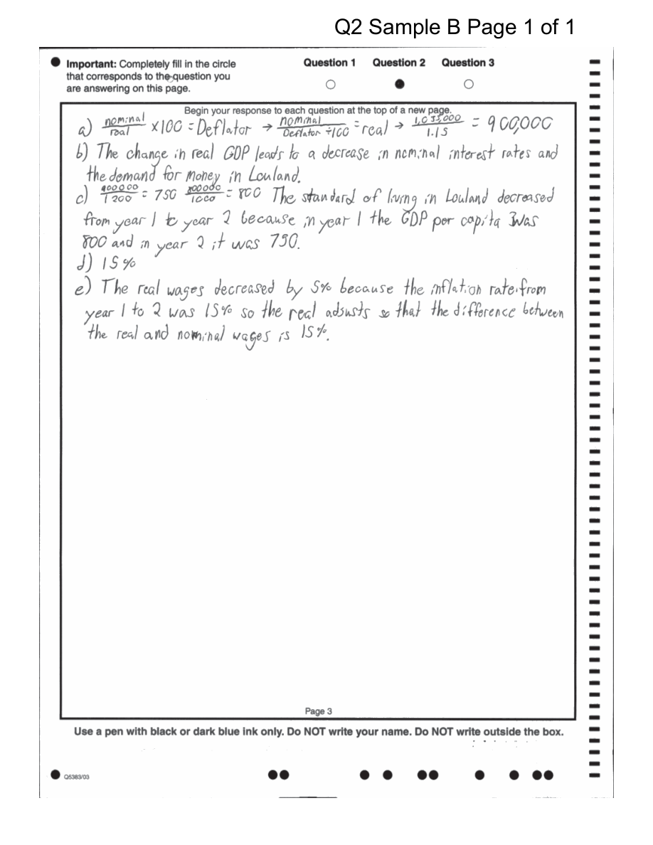
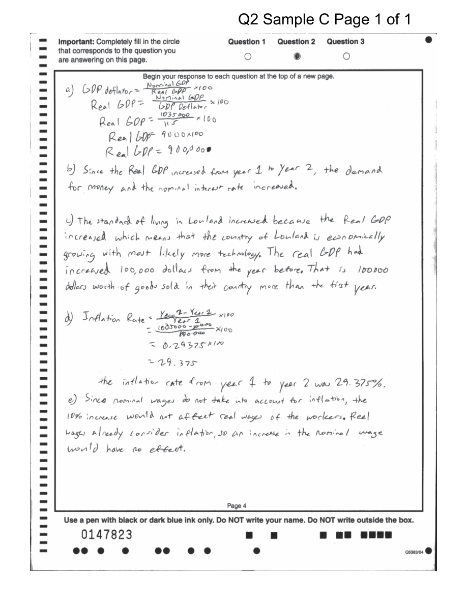
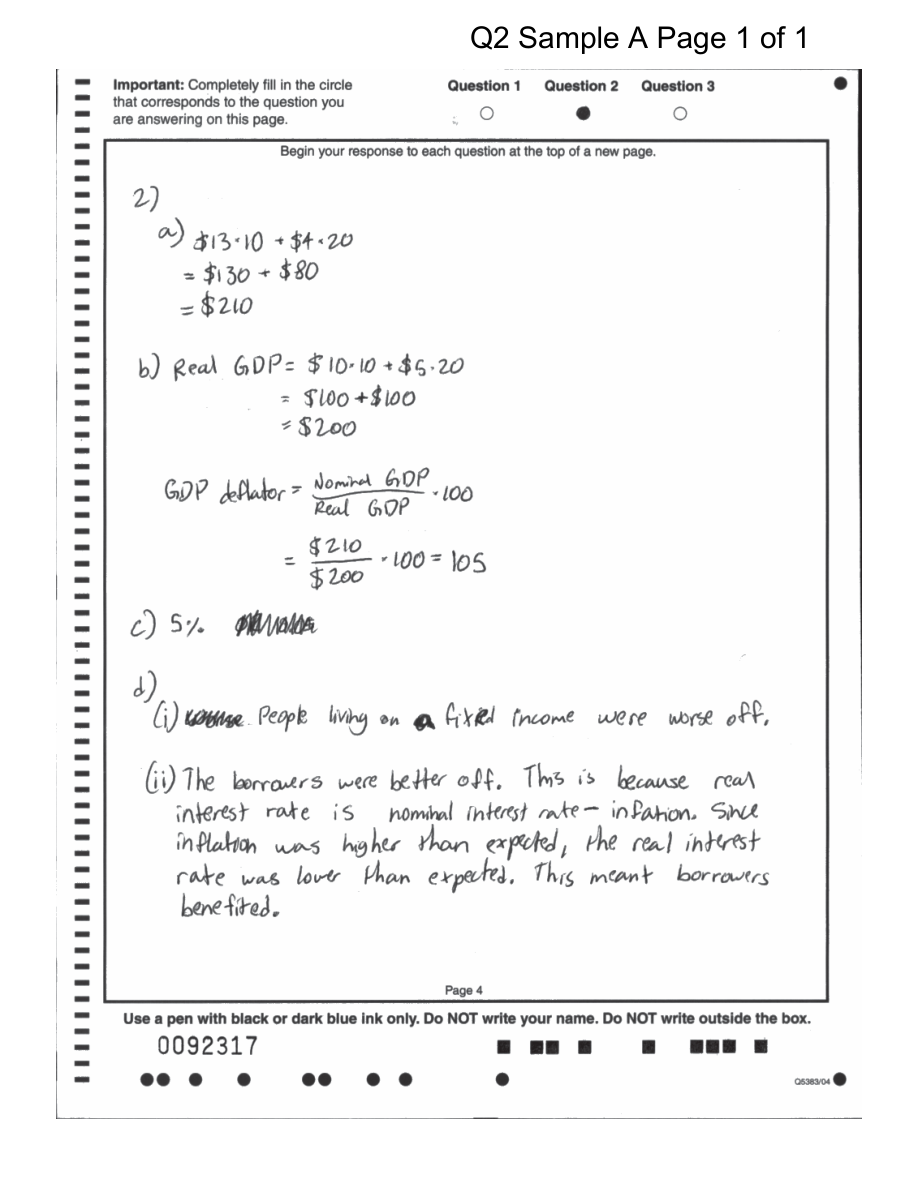
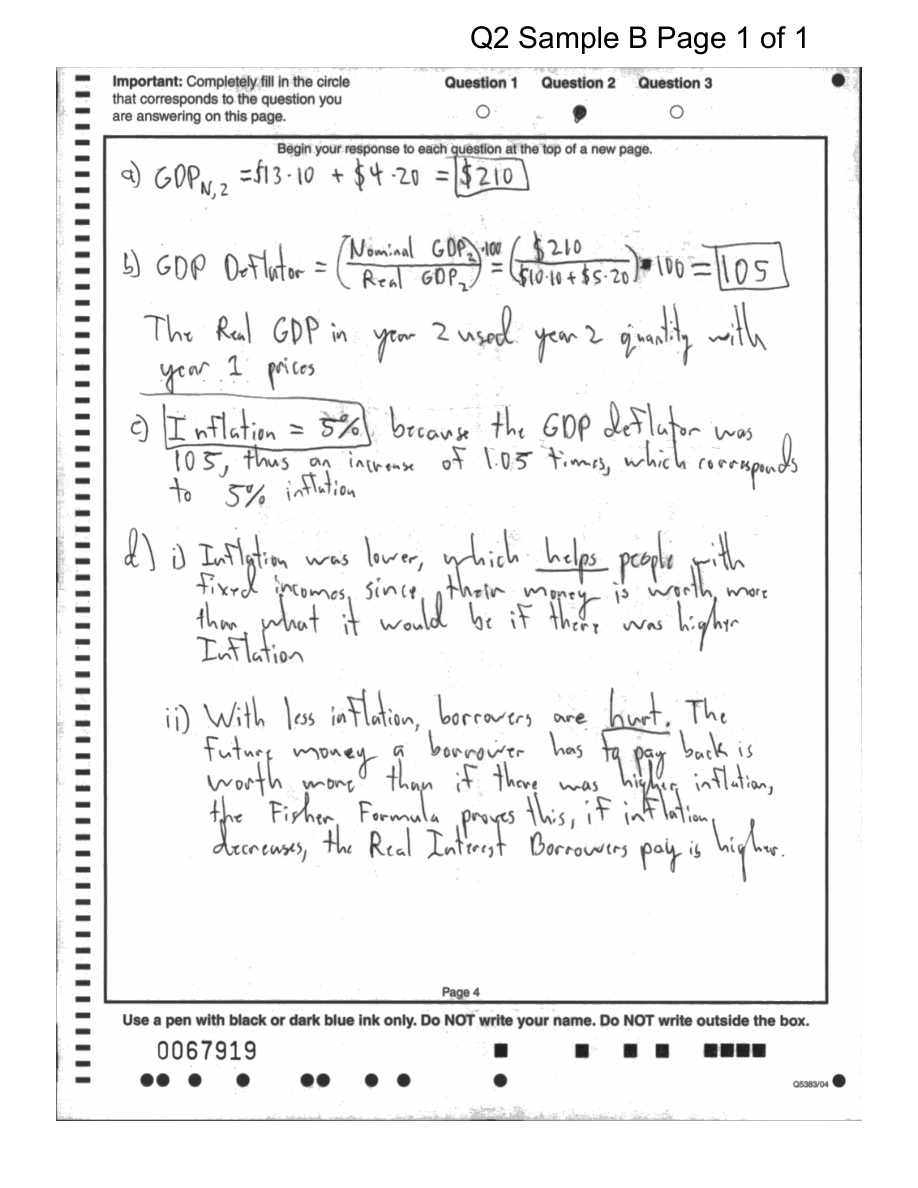
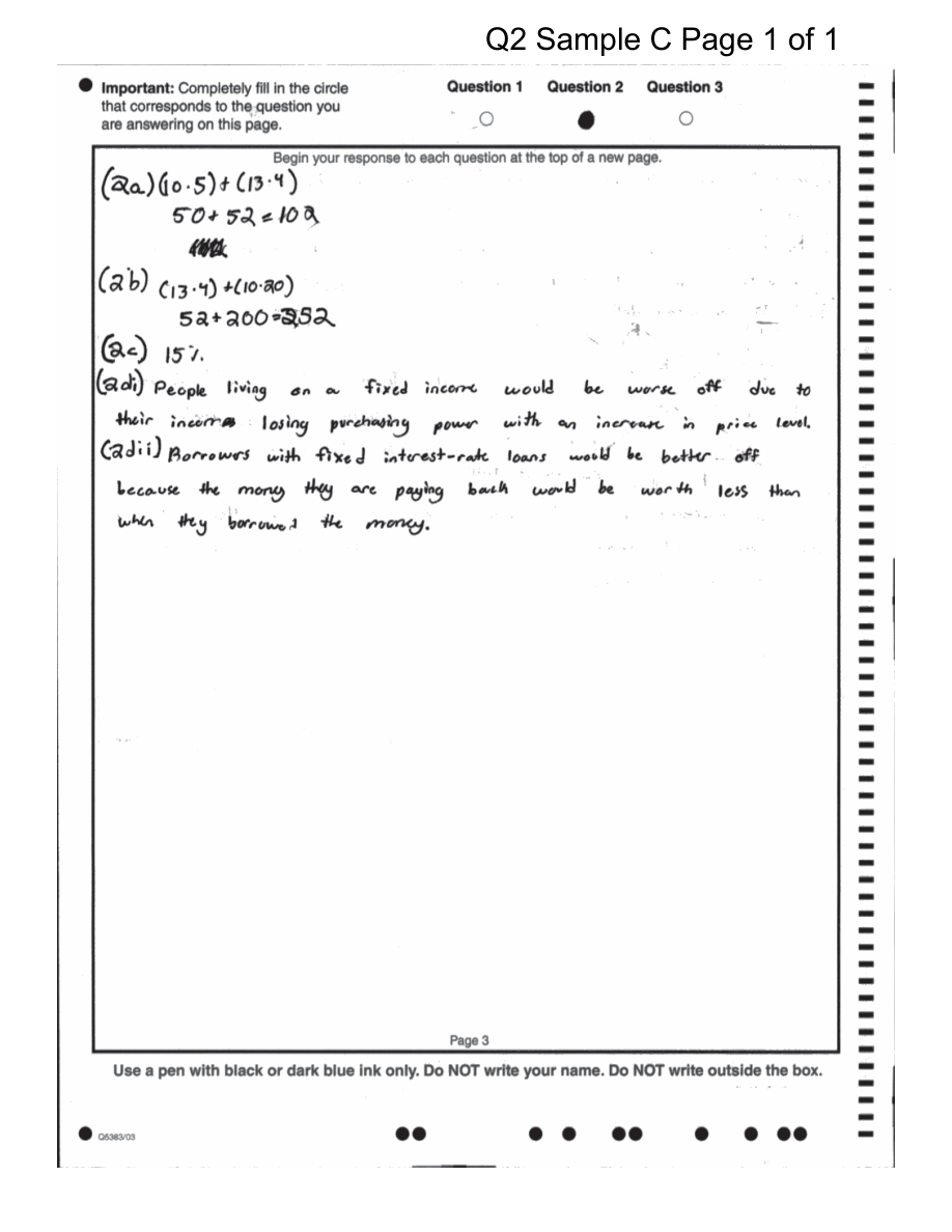
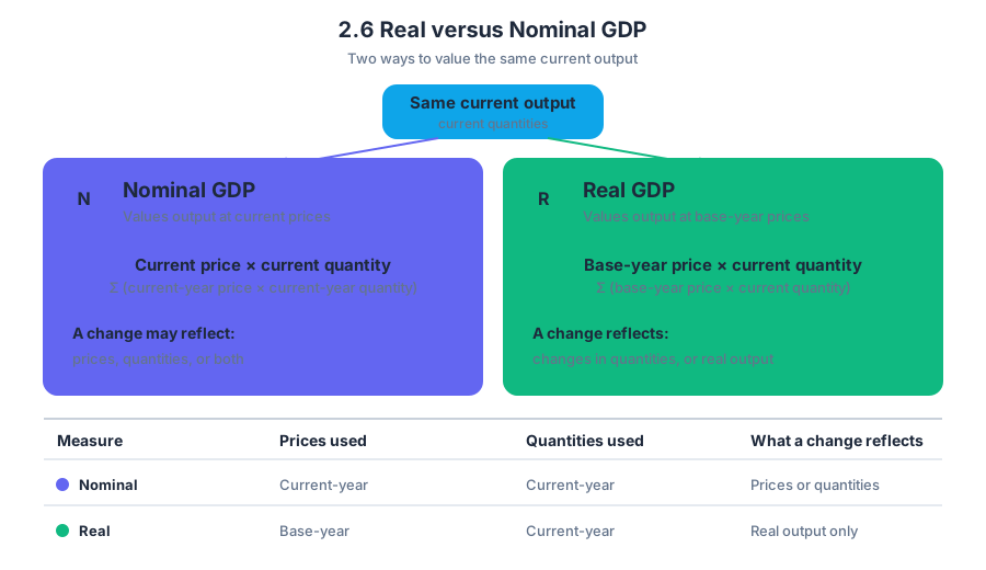
2.7 Business Cycles
An economy can grow while performing below its long-run potential, and it can shrink while still producing above trend. Business cycles describe the repeated fluctuations in economic activity over time—not simply whether actual output lies above or below a trend line.
2.7 Business Cycles
An economy can grow while performing below its long-run potential, and it can shrink while still producing above trend. Business cycles describe the repeated fluctuations in economic activity over time—not simply whether actual output lies above or below a trend line.
Business cycle: The recurring pattern of expansions and contractions in an economy’s level of economic activity.
The central diagnostic is therefore the direction of change in real output. When real GDP rises, the economy is generally in an expansion; when real GDP falls or weakens substantially, it is in a contraction. The economy moves through four commonly labeled points or phases: expansion, peak, contraction, and trough.
Reading the cycle: direction first, position second
A typical business-cycle diagram plots real GDP vertically and time horizontally. The long-run trend represents the economy’s rising productive capacity, while the actual-output line moves above and below that trend.
The actual-output line’s slope identifies the phase:
- Expansion: Actual real GDP is increasing.
- Peak: Economic activity reaches a temporary high point before turning downward.
- Contraction: Actual real GDP is decreasing or economic activity is weakening.
- Trough: Economic activity reaches a temporary low point before turning upward.
The distance between actual output and the long-run trend is a different idea. It describes the economy’s relative performance and is often connected to the output gap, the difference between actual output and potential or trend output. A negative output gap means actual output is below the relevant benchmark; a positive output gap means it is above it. Neither gap, by itself, determines whether the economy is expanding or contracting.
A four-point interpretation
Suppose an economy’s long-run trend rises steadily from $100$ to $120$ billion, while actual real GDP follows this path:
| Year | Actual real GDP | Direction of change | Business-cycle interpretation |
|---|---|---|---|
| $1$ | $100$ billion | — | Starting point |
| $2$ | $104$ billion | Rising | Expansion |
| $3$ | $108$ billion | Rising | Expansion |
| $4$ | $106$ billion | Falling | Contraction |
| $5$ | $103$ billion | Falling | Contraction |
| $6$ | $105$ billion | Rising | Recovery or expansion |
Even if the trend value in Year $4$ is $112$ billion, the economy is still in a contraction because actual GDP fell from $108$ billion to $106$ billion. Conversely, an economy could be expanding below trend if actual GDP rose from $90$ billion to $92$ billion while potential output rose from $100$ billion to $105$ billion.
Exam rule: Use the direction of actual economic activity to identify the business-cycle phase. Use the gap from trend to describe whether performance is relatively weak or strong.
Why business cycles matter
Business-cycle fluctuations affect employment, income, consumption, investment, and government budgets. During an expansion, firms typically sell more, hire more workers, and increase production. During a contraction, falling demand can reduce production and employment, while tax collections may decline and spending on income-support programs may rise.
Business cycles are not perfectly regular. Their length and severity vary because economies experience changing consumer confidence, business investment, financial conditions, policy actions, supply disruptions, and international shocks. A contraction caused by falling household spending need not look identical to one caused by a sudden increase in production costs.
Misconception check: “Below trend means contraction”
Named misconception — the trend-position error: A student sees actual GDP below the long-run trend and labels the economy a contraction. That conclusion is incomplete. If actual GDP is below trend but rising, the economy is expanding with a negative output gap; if actual GDP is above trend but falling, the economy is contracting with a positive output gap.
CED traceability: Topic 2.7 Business Cycles; Big Idea MEA; Skill Category 1: Principles and Models. The associated reasoning process is to identify the relevant macroeconomic model or pattern, interpret its variables, and use the model to explain an economic condition or predict what follows from a change.
Retrieval check
An economy’s actual real GDP increases from $500$ billion to $505$ billion while its potential output increases from $510$ billion to $520$ billion. Is the economy expanding or contracting, and is its output gap positive or negative?
Answer: It is expanding, because actual GDP increased. Its output gap is negative, because actual GDP remains below potential output. The phase comes from the direction of change; the gap comes from the position relative to potential output.
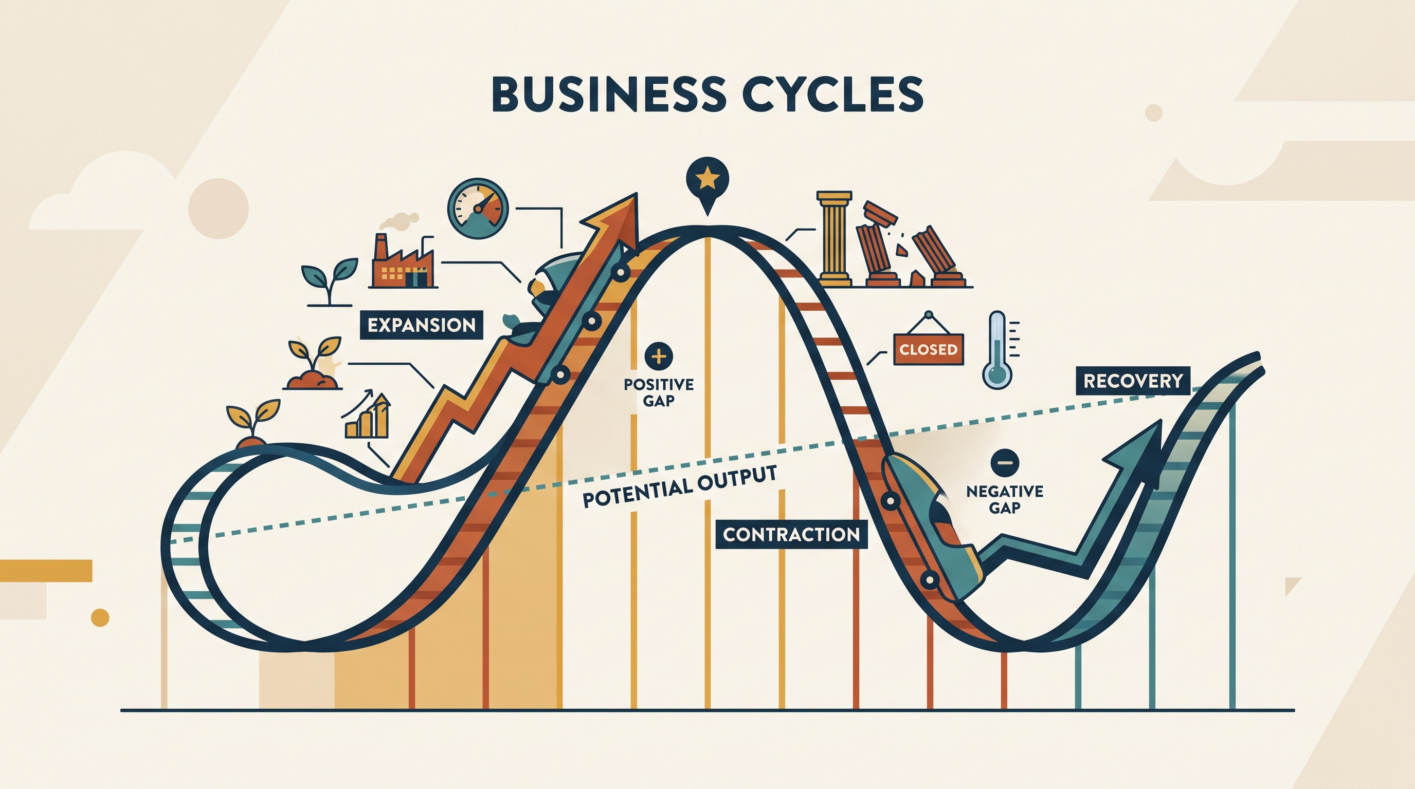
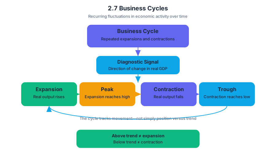
3.1 Aggregate Demand (AD)
Key concepts: Aggregate demand · Unemployment rate · Natural rate of unemployment · Recession · Expected inflation rate · Actual inflation rate · Maximum change in aggregate demand
Aggregate demand (AD) is the total quantity of final goods and services demanded in an economy at different overall price levels during a given period.
3.1 Aggregate Demand (AD)
Aggregate demand (AD) is the total quantity of final goods and services demanded in an economy at different overall price levels during a given period. It answers a macroeconomic question: How much real output will households, firms, the government, and foreign buyers collectively purchase?
The four components of aggregate demand are consumption, investment, government purchases, and net exports:
$$AD = C + I + G + NX$$
where $C$ is consumption spending, $I$ is investment spending, $G$ is government purchases, and $NX$ is net exports, calculated as exports minus imports.
The AD curve slopes downward because a lower overall price level generally encourages more consumption, increases the purchasing power of money, lowers interest rates through the money market, and makes domestic goods relatively less expensive to foreign buyers. A higher price level tends to produce the opposite effects.
Aggregate demand and the state of the economy
Suppose an economy has an actual unemployment rate of $7%$ and a natural rate of unemployment of $5%$. The natural rate is the unemployment rate that remains when the economy is producing at its sustainable, long-run level; it includes frictional and structural unemployment, but not cyclical unemployment.
Because the actual unemployment rate exceeds the natural rate,
$$7% - 5% = 2%$$
the economy has positive cyclical unemployment of $2$ percentage points. This condition indicates a recession: real output is below its potential or full-employment level, so the economy is experiencing a recessionary gap.
The causal chain is:
$$ \text{AD decreases} \rightarrow \text{real output decreases} \rightarrow \text{firms need fewer workers} \rightarrow \text{cyclical unemployment increases} $$
A recession does not mean that every industry is shrinking or that every worker is unemployed. It means that economy-wide production and employment are below their sustainable levels. A fall in aggregate demand is one important cause, although adverse short-run aggregate supply changes can also reduce output.
Expected and actual inflation
The expected inflation rate is the rate at which people and firms anticipate the overall price level will rise. The actual inflation rate is the rate at which the price level ultimately rises. Expectations influence wage contracts, borrowing decisions, pricing, and investment before the final inflation rate is known.
In a recession, weak aggregate demand places downward pressure on actual inflation. If households and firms expected inflation to be higher than the rate that actually occurs, then:
$$\text{Actual inflation} < \text{Expected inflation}$$
For example, if firms and workers expected prices to rise by $3%$, but weak demand causes prices to rise by only $1%$, actual inflation is below the expected inflation rate. This relationship is consistent with an economy operating to the right of its natural rate of unemployment on a short-run Phillips curve.
Misconception check — “A recession always means deflation.” A recession usually reduces the inflation rate relative to what was expected, but it does not necessarily make the price level fall. Prices may still increase, only more slowly than expected. A positive inflation rate can coexist with a recession.
From spending changes to changes in AD
A change in one component of spending shifts the AD curve. For instance, a $20 billion decrease in initial spending reduces aggregate demand. The maximum total change in AD depends on repeated rounds of spending, but the detailed multiplier mechanism belongs to Topic 3.2. Here, the essential point is that an initial spending change can produce a larger total change in equilibrium output and AD.
Using a marginal propensity to consume of $0.9$, the maximum change can be calculated as:
$$\text{Spending multiplier} = \frac{1}{1 - 0.9} = 10$$
$$\text{Maximum change in AD} = -$20\text{ billion} \times 10 = -$200\text{ billion}$$
The negative sign matters: the initial reduction in spending causes aggregate demand to decrease by a maximum of $$200$ billion. If the question instead supplies a different multiplier or a different marginal propensity to consume, use the values provided and show each substitution clearly.
AP skill connections
Topic 3.1 commonly assesses the following official skill categories:
- Skill 1: Principles and Models — identify aggregate demand and use the AD model to represent economy-wide spending.
- Skill 2: Interpretation — infer recessionary conditions by comparing actual unemployment with the natural rate and by comparing actual inflation with expected inflation.
- Skill 3: Manipulation — calculate a change in aggregate demand from an initial spending change and a supplied multiplier relationship.
- Skill 4: Graphing and Visuals — draw a correctly labeled AD curve with the price level on the vertical axis and real output on the horizontal axis; show a decrease in AD as a leftward shift.
Retrieval check: An economy has an actual unemployment rate of $7%$ and a natural rate of $5%$. Is it in a recession, and how should actual inflation compare with expected inflation if aggregate demand is weak?
Answer: Yes. Since actual unemployment exceeds the natural rate, the economy has cyclical unemployment and is in a recession. With weak aggregate demand, actual inflation is below the expected inflation rate.
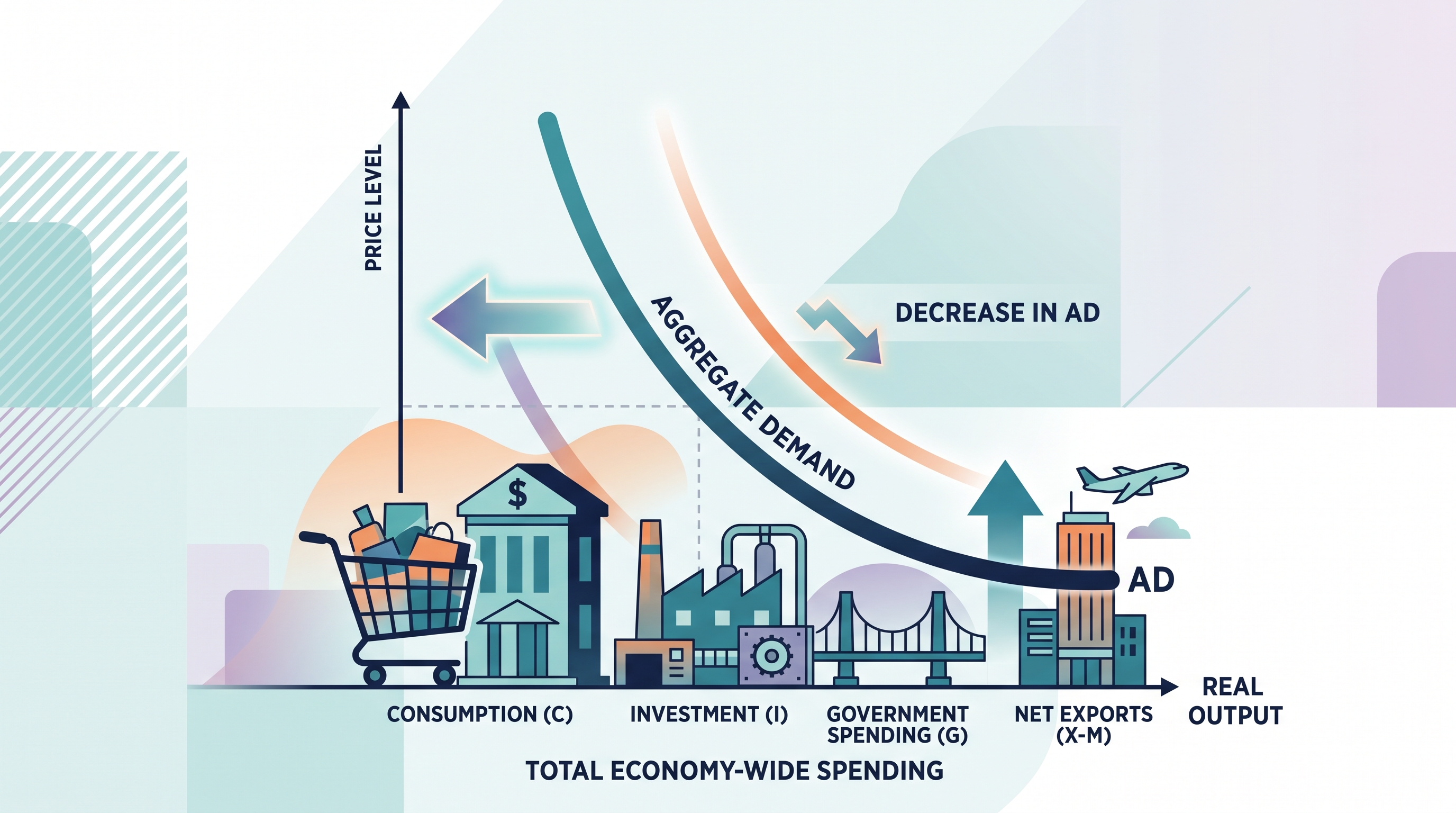
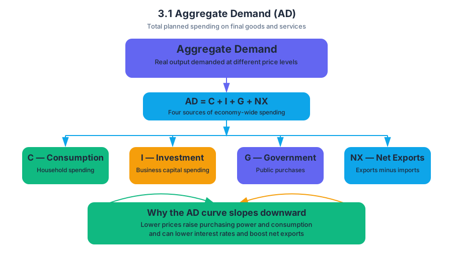
3.2 Multipliers
A $1 increase in spending can raise total real GDP by more than $1 because one person’s spending becomes another person’s income, which creates further rounds of spending.
3.2 Multipliers
A $1 increase in spending can raise total real GDP by more than $1 because one person’s spending becomes another person’s income, which creates further rounds of spending. This chain reaction is the multiplier effect.
The spending chain
Imagine that the government purchases $100 million of new public-transport equipment. The firms producing the equipment receive that $100 million as revenue and pay some of it to workers and suppliers. Those recipients spend part of their new income, creating income for others, who spend part of that income again.
The first round is always the largest. Each later round is smaller because households save part of their income rather than spend all of it. The marginal propensity to consume, or $MPC$, is the fraction of an additional dollar of disposable income that households spend; the marginal propensity to save, or $MPS$, is the fraction saved.
$$MPC + MPS = 1$$
If households spend $0.80 of every additional dollar, then $MPC = 0.8$ and $MPS = 0.2$. The spending multiplier is therefore:
$$\text{Spending multiplier} = \frac{1}{1-MPC} = \frac{1}{MPS}$$
$$\text{Spending multiplier} = \frac{1}{1-0.8} = \frac{1}{0.2}=5$$
Worked example: government purchases
Suppose real GDP is below potential output by $12$ billion. The government increases purchases by $3$ billion, and the economy’s $MPC$ is $0.75$.
$$\text{Spending multiplier}=\frac{1}{1-0.75}=4$$
$$\Delta \text{Real GDP}=4 \times $3\text{ billion}=$12\text{ billion}$$
The initial $3$-billion increase in government purchases produces a total $12$-billion increase in real GDP, exactly closing the output gap in this simplified model. The rounds are:
| Spending round | New spending |
|---|---|
| Initial government purchases | $$3.00$ billion |
| Round 2: $0.75 \times $3.00$ | $$2.25$ billion |
| Round 3: $0.75 \times $2.25$ | $$1.69$ billion |
| Later rounds | progressively smaller |
| Total effect | $$12.00$ billion |
In a complete macroeconomic model, the final effect may be smaller because households may save, taxes may reduce disposable income, imports may send spending abroad, and higher interest rates may reduce private investment. The multiplier is therefore a calculated model result, not a guarantee that every dollar produces the same final increase.
Tax changes use a different multiplier
A tax change affects GDP indirectly. When taxes fall, disposable income rises; households then spend only the fraction represented by the $MPC$. Consequently, the tax multiplier is smaller in absolute value than the spending multiplier:
$$\text{Tax multiplier}=\frac{-MPC}{1-MPC}$$
With $MPC=0.75$:
$$\text{Tax multiplier}=\frac{-0.75}{0.25}=-3$$
A tax cut of $$4$ billion changes real GDP by:
$$\Delta \text{Real GDP}=(-3)(-$4\text{ billion})=$12\text{ billion}$$
The negative sign means that a tax increase decreases aggregate demand, while a tax cut increases it. Notice that a $$4$-billion tax cut and a $$3$-billion increase in government purchases have the same total effect in this example, because government purchases enter aggregate demand directly but tax changes first pass through household spending.
Key insight: For an equal-sized change, the government-purchases multiplier is larger than the tax multiplier because households do not spend all of a tax change.
AP skills in action
Topic identifier: 3.2 Multipliers. This topic is assessed through the official skill categories Skill Category 1: Principles and Models, Skill Category 2: Interpretation, Skill Category 3: Manipulation, and Skill Category 4: Graphing and Visuals.
- Skill Category 1: Principles and Models: identify whether a policy changes government purchases, taxes, or another component of spending, then select the appropriate multiplier.
- Skill Category 2: Interpretation: explain why successive rounds of spending become smaller and connect the result to changes in real GDP.
- Skill Category 3: Manipulation: calculate $MPC$, $MPS$, the spending multiplier, the tax multiplier, or the required policy change.
- Skill Category 4: Graphing and Visuals: show the resulting shift in aggregate demand and identify the change in equilibrium real GDP when a multiplier problem supplies an AD–AS diagram.
Misconception check
Misconception: “The multiplier is always larger than $1$.” The spending multiplier exceeds $1$ only when $0<MPC<1$. A larger $MPC$ produces a larger multiplier because less income leaks into saving. Also, the tax multiplier is negative, not positive: a tax increase reduces disposable income and decreases aggregate demand.
Retrieval check
If $MPC=0.6$ and government purchases rise by $$5$ billion, calculate the change in real GDP.
$$\text{Spending multiplier}=\frac{1}{1-0.6}=2.5$$
$$\Delta \text{Real GDP}=2.5 \times $5\text{ billion}=\boxed{$12.5\text{ billion}}$$

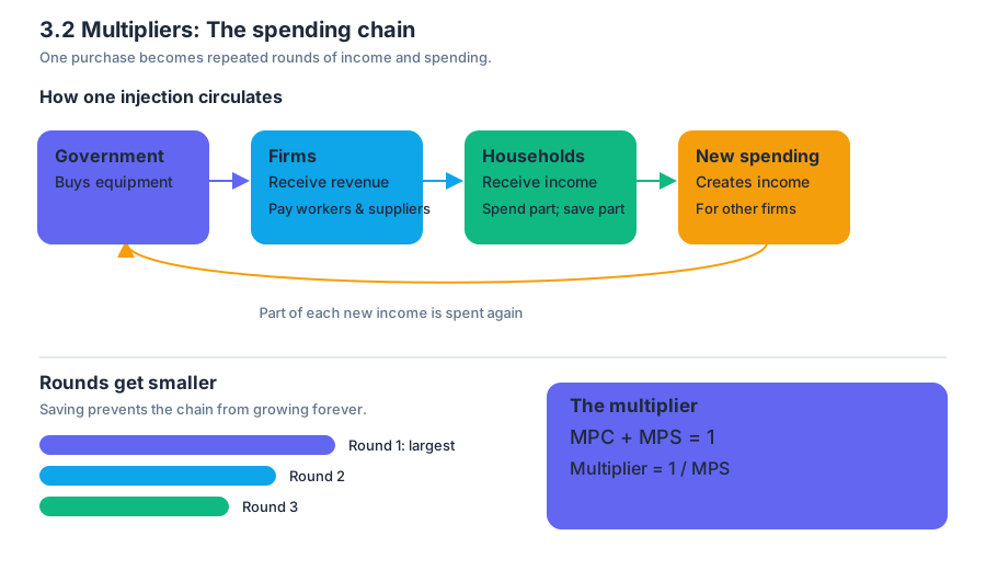
3.3 Short-Run Aggregate Supply (SRAS)
Key concepts: Short-run aggregate supply (SRAS) curve · Relationship between the price level and aggregate output · Sticky wages and fixed input prices · Movement along the SRAS curve · Shifts in the SRAS curve · Positive and negative supply shocks · Aggregate-demand shocks · Short-run equilibrium and full-employment output · Inflationary and recessionary gaps · Effects on output, employment, and the price level
Why can firms produce more when the economy-wide price level rises, even though the economy’s technology and resources have not changed? In the short run, many production costs—especially wages and some input prices—do not adjust immediately.
3.3 Short-Run Aggregate Supply (SRAS)
Why can firms produce more when the economy-wide price level rises, even though the economy’s technology and resources have not changed? In the short run, many production costs—especially wages and some input prices—do not adjust immediately. That temporary mismatch makes the short-run aggregate supply (SRAS) curve upward-sloping.
Short-run aggregate supply (SRAS) describes the relationship between the economy-wide price level and the quantity of goods and services firms are willing and able to produce in the short run.
The vertical axis of the AD–AS graph measures the price level, and the horizontal axis measures real output, usually labeled real GDP or $Y$. SRAS slopes upward: a higher price level is associated with a greater quantity of output supplied in the short run.
Why SRAS slopes upward
Suppose a bakery agrees to pay its workers a wage of $15 per hour for the next year. If the prices of the bakery’s products rise while that wage remains fixed, each loaf becomes more profitable to produce. The bakery responds by increasing production and hiring more workers. Across the economy, this produces the upward-sloping SRAS curve.
The key mechanism is sticky wages: nominal wages are slow to change. Some other input prices may also be fixed temporarily because of contracts, menus, leases, or delayed information. Therefore, when the price level rises, firms’ selling prices may increase before their production costs do, encouraging greater real output and employment.
Essential Knowledge MOD-2.C.2: The SRAS curve is upward-sloping because wages and some input prices are sticky or fixed in the short run. This is a short-run relationship—not a claim that firms can permanently increase output merely by raising prices.
Movement along SRAS versus a shift
A movement along the SRAS curve occurs when the price level changes because aggregate demand changes. The SRAS curve itself remains in place. For example, a positive aggregate-demand shock shifts AD rightward; the new equilibrium moves upward and rightward along the existing SRAS curve, raising the price level, real output, and employment in the short run.
Conversely, a negative aggregate-demand shock shifts AD leftward. The economy moves downward and leftward along SRAS, reducing the price level, real output, and employment in the short run.
| Event | Graphical change | Short-run result |
|---|---|---|
| Positive AD shock | AD shifts right | Price level rises; output and employment rise |
| Negative AD shock | AD shifts left | Price level falls; output and employment fall |
| Positive SRAS shock | SRAS shifts right | Price level falls; output and employment rise |
| Negative SRAS shock | SRAS shifts left | Price level rises; output and employment fall |
Essential Knowledge MOD-2.C.3: Any factor that changes production costs—such as input prices or inflationary expectations—shifts SRAS. A change in the price level alone does not shift SRAS; it causes movement along the curve.
Supply shocks: good news and bad news
A positive SRAS shock lowers firms’ production costs. Examples include cheaper energy, improved production technology, or lower expected inflation. SRAS shifts right, increasing short-run output and employment while lowering the price level.
A negative SRAS shock raises production costs. A sudden increase in oil prices, for instance, makes transportation and manufacturing more expensive. SRAS shifts left, decreasing output and employment while raising the price level—a difficult combination often called stagflation.
Output gaps and short-run equilibrium
Short-run equilibrium occurs where AD and SRAS intersect, consistent with Essential Knowledge MOD-2.G.1. That equilibrium output may be below, at, or above the economy’s short-run full-employment level of output.
- Below full employment: a negative, or recessionary, output gap; unemployment is elevated.
- At full employment: output equals the full-employment level.
- Above full employment: a positive, or inflationary, output gap; upward pressure on prices is present.
A positive AD shock can push output above full employment, creating an inflationary situation. A negative AD shock can push output below full employment, creating a recessionary situation. These gaps describe the economy’s position relative to full employment; they are not themselves shifts of SRAS.
Worked example
Assume the economy begins at the intersection of $AD_1$ and $SRAS_1$, with output below full employment. Consumer confidence rises, increasing consumption and shifting AD rightward from $AD_1$ to $AD_2$. The economy moves along $SRAS_1$: the price level rises from $PL_1$ to $PL_2$, output rises from $Y_1$ to $Y_2$, and employment increases.
Now instead assume a major drought raises food prices and production costs. SRAS shifts left from $SRAS_1$ to $SRAS_2$. The new equilibrium has a higher price level and lower real output. The correct explanation must include the complete chain: higher input prices $\rightarrow$ higher production costs $\rightarrow$ SRAS shifts left $\rightarrow$ output and employment fall while the price level rises.
Misconception check
Common misconception: “Any increase in the price level shifts SRAS.”
Correction: An increase in the price level caused by higher aggregate demand creates a movement along SRAS. SRAS shifts only when a determinant of production costs changes, such as wages, input prices, technology, or inflationary expectations.
AP skill in action
This topic most directly uses Skill 1—Principles and Models, to identify the SRAS mechanism; Skill 2—Interpretation, to infer changes in output, employment, and the price level; and Skill 4—Graphing and Visuals, to draw labeled AD–AS graphs, distinguish movements from shifts, and identify output gaps. The central reasoning process is always causal: identify the shock, determine which curve changes, locate the new equilibrium, and state all affected macroeconomic variables.
Retrieval check: If input prices fall while aggregate demand is unchanged, does the economy move along SRAS or does SRAS shift? What happens to the price level, output, and employment?
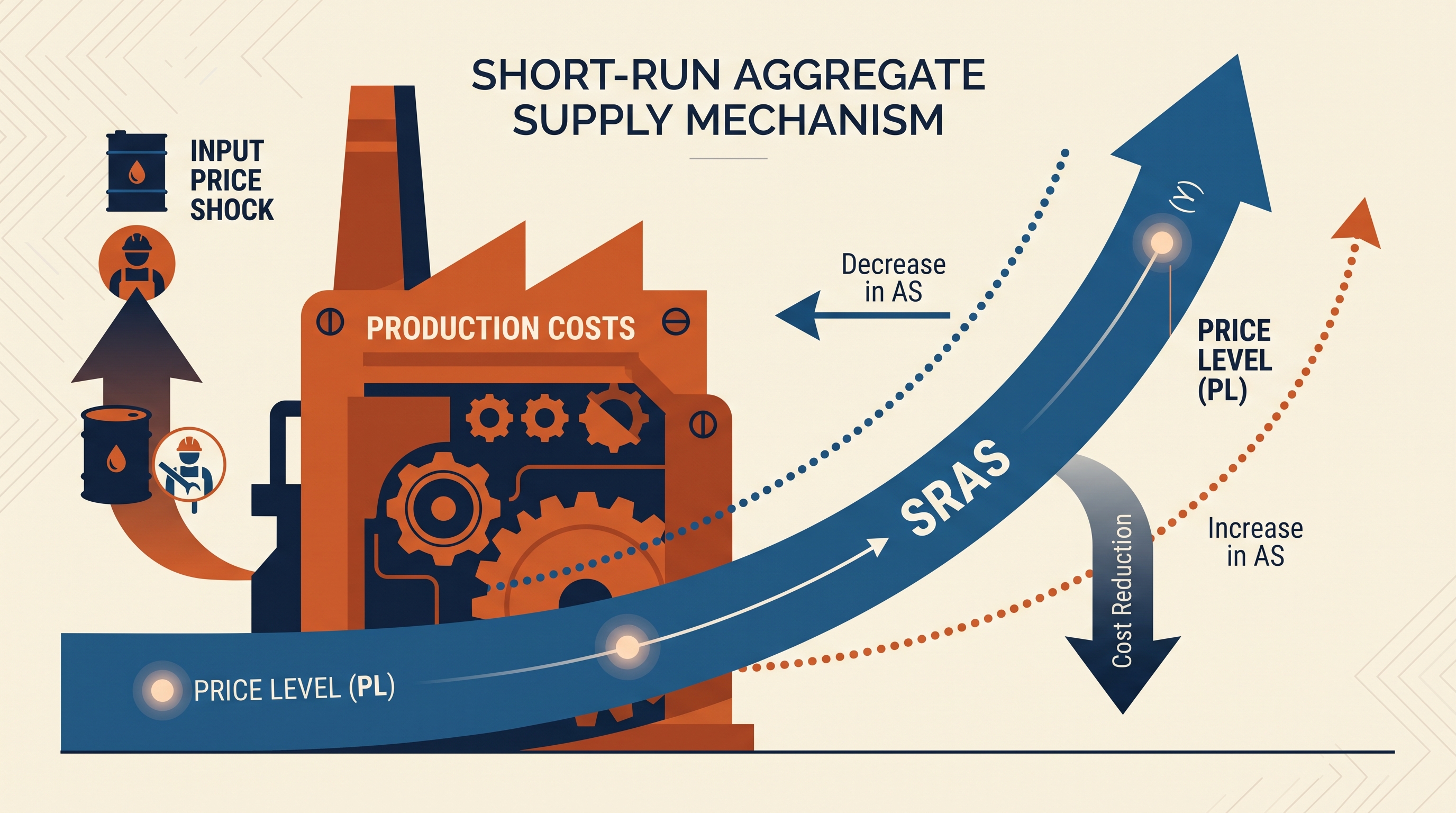
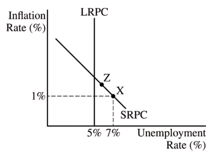
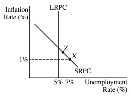
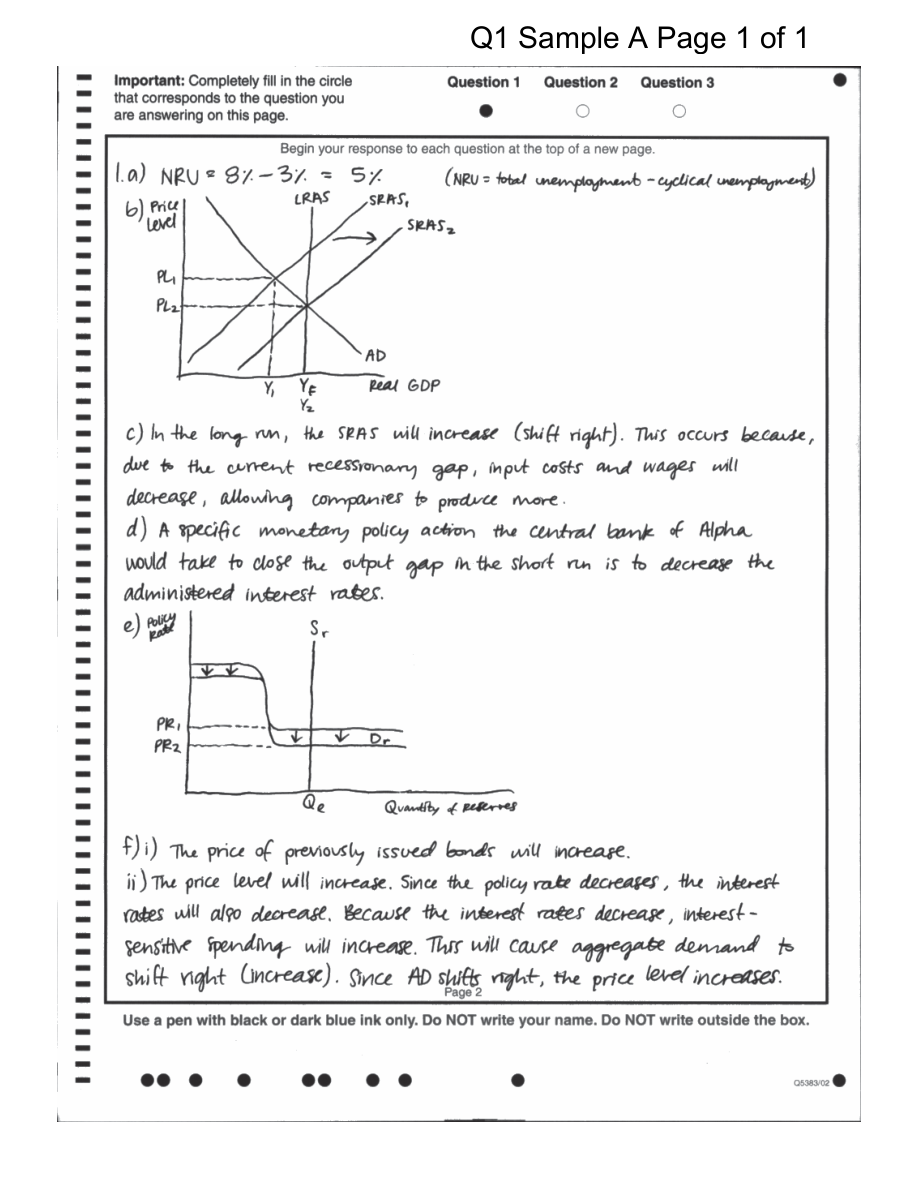
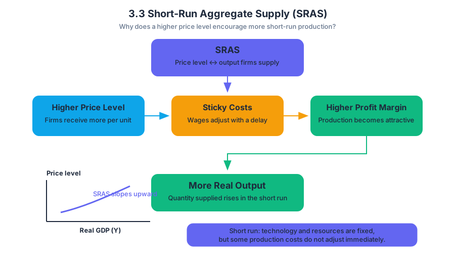
3.4 Long-Run Aggregate Supply (LRAS)
Key concepts: Long-run aggregate supply (LRAS) · Maximum sustainable capacity · Full-employment level of output · Production possibilities curve (PPC) · Flexible wages and prices in the long run · Fixed input prices in the short run · Long-run equilibrium price level and output level · Economic growth · Infrastructure and technology investment · Natural rate of unemployment
Why can an economy temporarily produce above or below its sustainable capacity, yet eventually return to a particular level of output? The answer is the long-run aggregate supply (LRAS) curve: it identifies the economy’s full-employment level of real output after wages and prices have had time to adjust completely.
3.4 Long-Run Aggregate Supply (LRAS)
Why can an economy temporarily produce above or below its sustainable capacity, yet eventually return to a particular level of output? The answer is the long-run aggregate supply (LRAS) curve: it identifies the economy’s full-employment level of real output after wages and prices have had time to adjust completely.
Investigative question: If the price level changes, why does the economy’s long-run productive capacity not automatically change?
The long run is defined by flexibility
The short run and long run are distinguished by how quickly prices respond, not by a fixed number of months or years. In the short run, some input prices—especially wages and contracted costs—are fixed or “sticky.” In the long run, all wages and prices are fully flexible (MOD-2.E.1).
This distinction matters because a business may face higher product prices before it can renegotiate worker wages or supplier contracts. During that interval, production and employment can change. Once wages and other input prices fully adjust, however, firms no longer have a lasting reason to employ resources beyond the economy’s sustainable capacity.
What LRAS measures
The long-run aggregate supply curve shows the quantity of real output an economy can produce when all resources are fully employed. This quantity is called the full-employment level of output, or $Y_F$. It is also the economy’s maximum sustainable capacity: the total output an economic system can produce over a period of time when its resources are fully employed (MOD-2.F.1).
On an AD–AS graph, the LRAS curve is vertical at $Y_F$ (MOD-2.F.2). The vertical shape means that changes in the price level alone do not permanently change the economy’s full-employment output. The horizontal axis measures real output, while the vertical axis measures the price level.
$$ \text{LRAS: } Y = Y_F $$
The LRAS curve resembles the production possibilities curve (PPC) because both models represent maximum sustainable capacity. The PPC displays the maximum combinations of two goods that can be produced with fully employed resources; LRAS compresses the economy’s productive possibilities into one macroeconomic output measure.
Principles and Models (1.A): Describe economic concepts, principles, or models. A complete description must do more than state “LRAS is vertical.” It must connect verticality to flexible wages and prices, connect $Y_F$ to full employment, and explain why a change in productive resources—not merely a change in the price level—moves LRAS.
Shock and long-run adjustment
Suppose households suddenly reduce consumption. Aggregate demand falls, and in the short run real output and employment decrease while the price level falls. Because wages and other input prices do not immediately adjust, firms can temporarily produce at an output level below $Y_F$.
Over time, weaker demand reduces pressure on labor and product markets. Nominal wages and other input prices fall, lowering firms’ production costs. Short-run aggregate supply shifts rightward until output returns to $Y_F$; unemployment returns to its natural rate, the rate associated with normal frictional and structural unemployment (MOD-2.I.1).
The same logic works after an adverse short-run aggregate supply shock, such as a sudden increase in energy costs. Output initially falls and the price level rises. If no government policy intervenes, wages and other input prices eventually adjust, allowing short-run aggregate supply to move back and restoring full employment.
Because wages and prices fully adjust in the long run, there is no permanent long-run trade-off between inflation and unemployment (MOD-2.E.1). Expansionary demand can temporarily increase output and reduce unemployment, but once expectations, wages, and prices adjust, output returns to $Y_F$ rather than remaining permanently above it.
Worked example: identifying the adjustment
An economy begins in long-run equilibrium at $Y_F = 500$ billion of real output. A fall in consumer confidence shifts AD left, moving short-run output to $470$ billion. The economy now has a recessionary gap of $30$ billion:
$$ \text{Recessionary gap} = Y_F - Y_{\text{short run}} $$
$$ \text{Recessionary gap} = $500\text{ billion} - $470\text{ billion} = $30\text{ billion} $$
With no policy action, falling wages and input prices shift SRAS right. The final long-run result is real output of $500$ billion, unemployment at its natural rate, and a lower price level than before the demand shock. The shock changes the price level temporarily and output temporarily, but it does not change $Y_F$.
When LRAS shifts
A shift in LRAS means that the economy’s full-employment level of output has changed (MOD-2.I.2). LRAS shifts right when productive capacity expands—for example, through improved technology, a larger or better-trained labor force, additional capital, or infrastructure that makes production more efficient.
Government policies can therefore affect potential output. Public investment in transportation networks, energy systems, communications, education, or technology can increase long-run productive capacity. Supply-side fiscal policies may affect aggregate supply and potential output in both the short run and the long run, although the timing and size of those effects depend on the policy.
Misconception check
Misconception: “A higher price level shifts LRAS right.” Correction: a higher price level is a movement along the vertical LRAS curve, not a change in productive capacity. LRAS shifts only when the full-employment quantity of output changes.
Misconception: “Full employment means zero unemployment.” Correction: at $Y_F$, the economy still has its natural rate of unemployment. Full employment means no cyclical unemployment, not that every person is employed at every moment.
Retrieval check
An economy’s output falls below $Y_F$ after an aggregate demand shock. What restores full employment in the absence of policy, and what happens to unemployment in the long run? The essential chain is: flexible wages and prices $\rightarrow$ lower input costs $\rightarrow$ SRAS shifts right $\rightarrow$ output returns to $Y_F$ $\rightarrow$ unemployment returns to its natural rate.
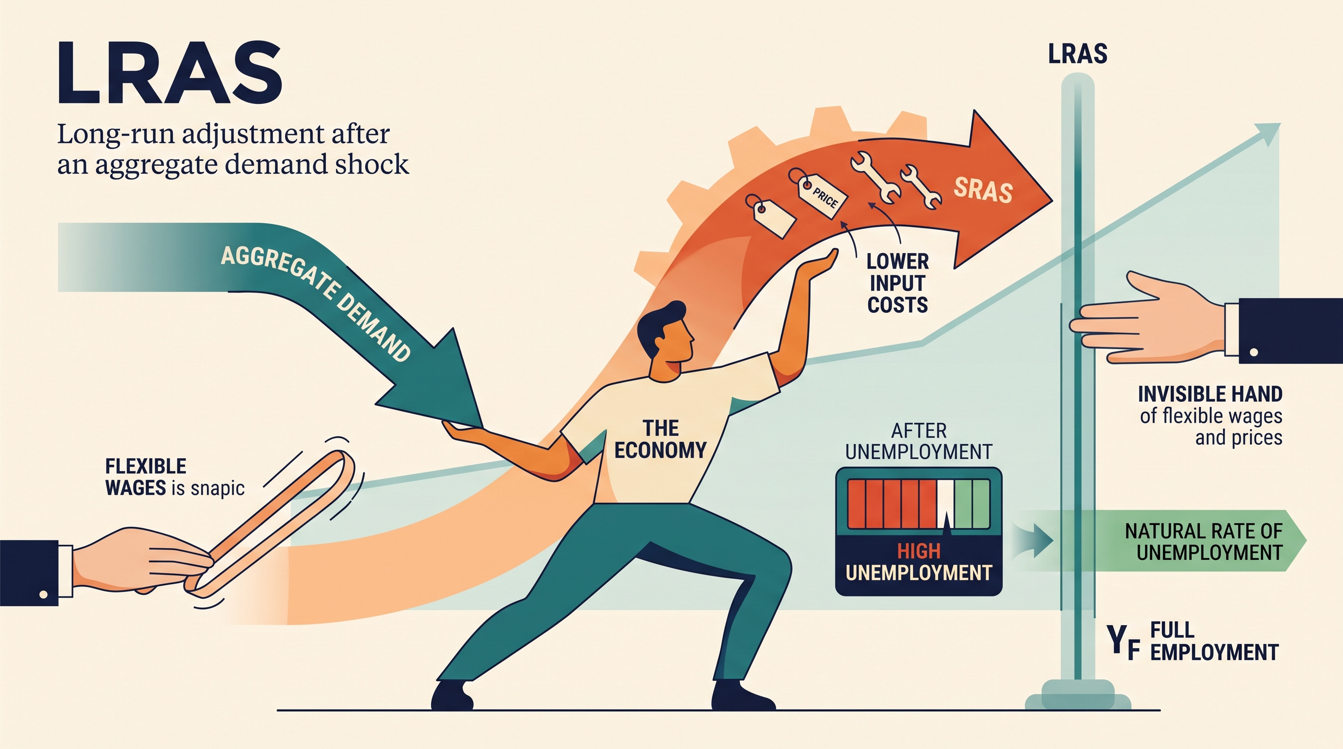
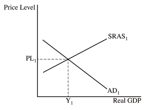
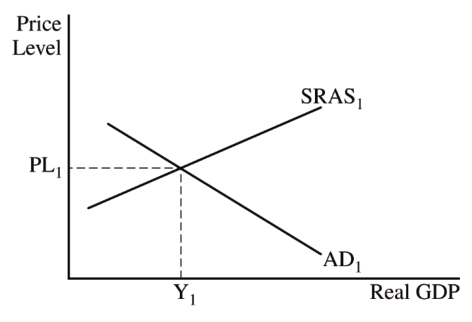
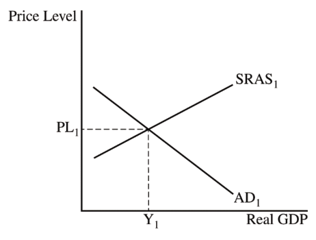
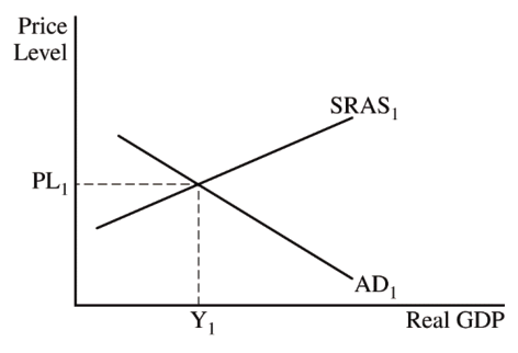
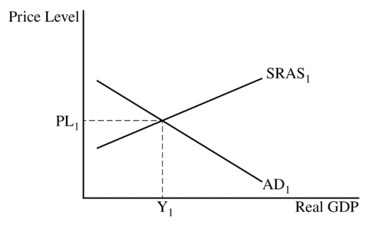
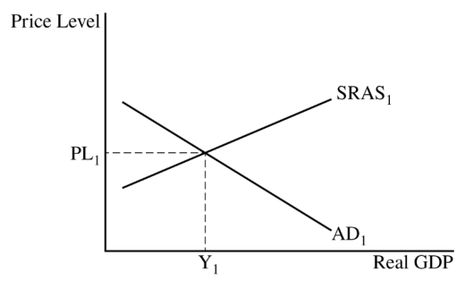
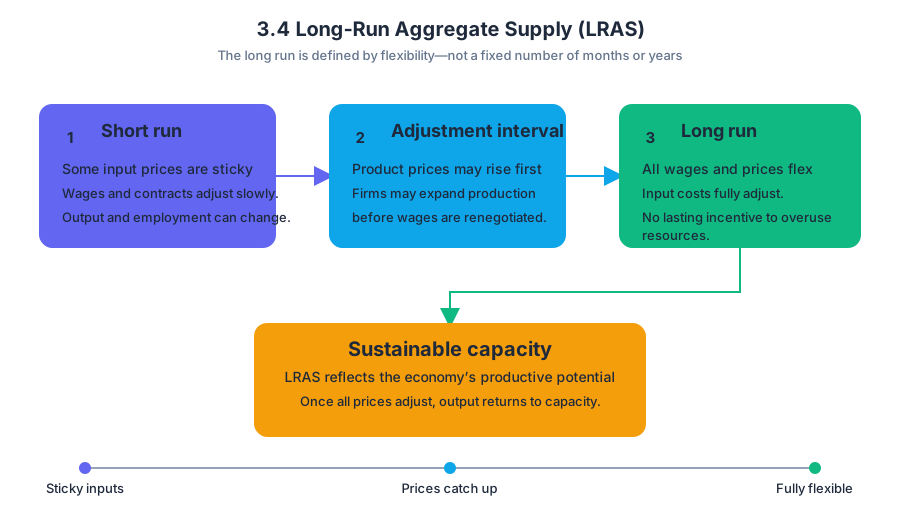
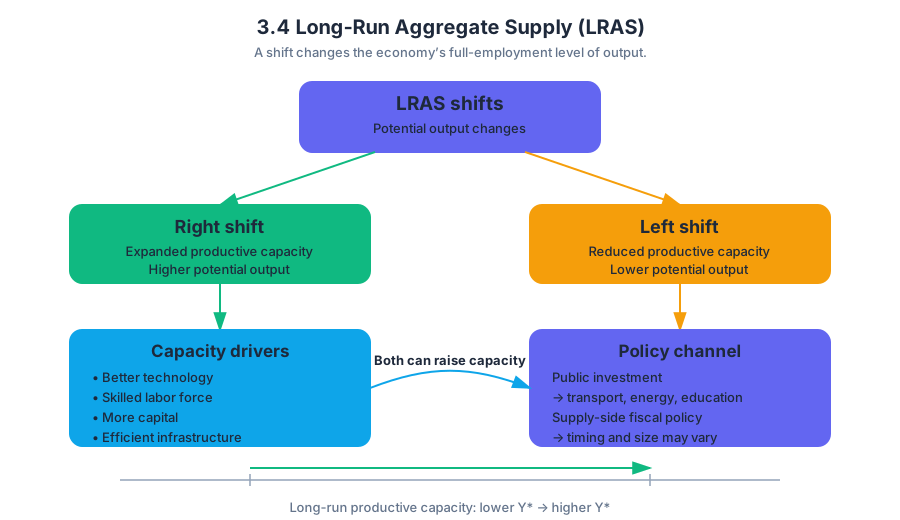
3.5 Equilibrium in the Aggregate Demand–Aggregate Supply (AD–AS) Model
Key concepts: Aggregate Demand–Aggregate Supply (AD–AS) model · Equilibrium in the AD–AS model · Aggregate demand · Aggregate supply · Macroeconomic indicators · Gross domestic product (GDP) · Real GDP · GDP deflator · Movement along a curve versus shifts of a curve · Accurately labeled economic graphs
The AD–AS model shows how an economy’s overall price level and real output are determined together. Its central question is simple: Where do the economy’s desired purchases meet the economy’s willingness to produce?
3.5 Equilibrium in the Aggregate Demand–Aggregate Supply (AD–AS) Model
The AD–AS model shows how an economy’s overall price level and real output are determined together. Its central question is simple: Where do the economy’s desired purchases meet the economy’s willingness to produce?
Learning Objective MOD-3.E: Explain how equilibrium in the aggregate demand–aggregate supply model represents an economy’s performance. Essential Knowledge MOD-3.E.1: The AD–AS model represents the relationship between the price level and real gross domestic product.
Reading the AD–AS equilibrium
Aggregate demand, or $AD$, is the total quantity of domestically produced final goods and services demanded at different price levels. It combines consumption, investment, government spending, and net exports:
$$AD = C + I + G + NX$$
Aggregate supply describes the total quantity of goods and services firms are willing and able to produce at different price levels. In the short run, the relevant curve is short-run aggregate supply, or $SRAS$.
Equilibrium in the AD–AS model occurs where the $AD$ curve intersects the $SRAS$ curve. At that point, planned spending equals actual production.
The horizontal axis must measure real GDP, also written as real output $Y$. The vertical axis must measure the price level, often written as $PL$. The equilibrium intersection identifies both the economy’s current real output, such as $Y_1$, and its current price level, such as $PL_1$.
Businesses influence aggregate demand through investment and production decisions; the government affects it through purchases, taxes, and transfers; and the rest of the world affects it through exports, imports, exchange rates, and international income. The model therefore connects household, business, government, and international activity in one economy-wide picture.
Movement versus shift
A change in the price level causes a movement along an existing $AD$ or $SRAS$ curve. A change in one of the determinants other than the price level causes the entire curve to shift.
| Change | Graphical result | Example |
|---|---|---|
| Price level rises | Movement upward along $AD$ | Households purchase less real output because purchasing power and interest-sensitive spending change |
| Consumption changes for a reason other than $PL$ | Shift of $AD$ | Consumer confidence increases |
| Input prices change | Shift of $SRAS$ | Energy costs rise |
| Price level falls | Movement downward along $SRAS$ | Firms respond to the lower overall selling-price level |
Misconception check — “Any change in output shifts $AD$.” Not necessarily. If the price level changes and the economy moves to another point on the same curve, that is a movement along the curve. A shift requires a change in a determinant such as consumption, investment, government spending, net exports, resource prices, or productivity.
Using macroeconomic indicators
The equilibrium output shown in the model is measured with real GDP, which values current production using prices from a base year. Real GDP is therefore designed to measure changes in production while removing the effect of changing prices. Nominal GDP uses current prices, so it can rise because the economy produces more, prices rise, or both.
The GDP deflator measures the price level of all final goods and services included in GDP:
$$GDP\ deflator = \frac{Nominal\ GDP}{Real\ GDP} \times 100$$
For example, suppose nominal GDP is $$1{,}200$ billion and real GDP is $$1{,}000$ billion. Then:
$$GDP\ deflator = \frac{1{,}200}{1{,}000}\times100 = 120$$
A deflator of $120$ means that the prices of domestically produced final goods and services are $20%$ higher than in the base year. It does not mean that real output is $20% higher.
Gaps and the business cycle
Using the LRAS benchmark from Section 3.4, compare the AD–SRAS equilibrium output with full-employment output $Y_F$. If equilibrium output is below $Y_F$, the economy has a recessionary gap and typically elevated cyclical unemployment. If equilibrium output is above $Y_F$, it has an inflationary gap, meaning short-run output exceeds its full-employment benchmark.
Suppose an economy’s equilibrium is at $Y_1$, while the benchmark is $Y_F$, with $Y_1>Y_F$. The graph identifies an inflationary gap; macroeconomic indicators would likely show output above sustainable full-employment production and pressure on the price level. If instead $Y_1<Y_F$, the economy is operating below capacity, consistent with a downturn in the business cycle.
Worked interpretation: A decline in business investment reduces one component of $AD$. On the graph, locate the new $AD$–$SRAS$ intersection and read the two coordinates: the new equilibrium real GDP and price level. The correct explanation must include the causal chain: lower investment $\rightarrow$ lower aggregate demand $\rightarrow$ lower equilibrium real output and price level, assuming an unchanged $SRAS$ curve.
AP reasoning and retrieval check
This topic directly develops Skill Category 1: Principles and Models, especially defining and explaining the AD–AS model; Skill Category 2: Interpretation, by reading GDP, real GDP, and the GDP deflator; and Skill Category 4: Graphing and Visuals, especially MOD-2.A.2 and MOD-2.A.3, which require an accurately labeled economic graph and an explanation of the relationship represented. The graph must show $PL$ and real GDP on the axes, correctly labeled $AD$ and $SRAS$ curves, and a clearly marked equilibrium.
Retrieval check: If nominal GDP rises while real GDP remains constant, what must happen to the GDP deflator? If the $AD$–$SRAS$ intersection lies left of $Y_F$, name the gap and the likely business-cycle condition.
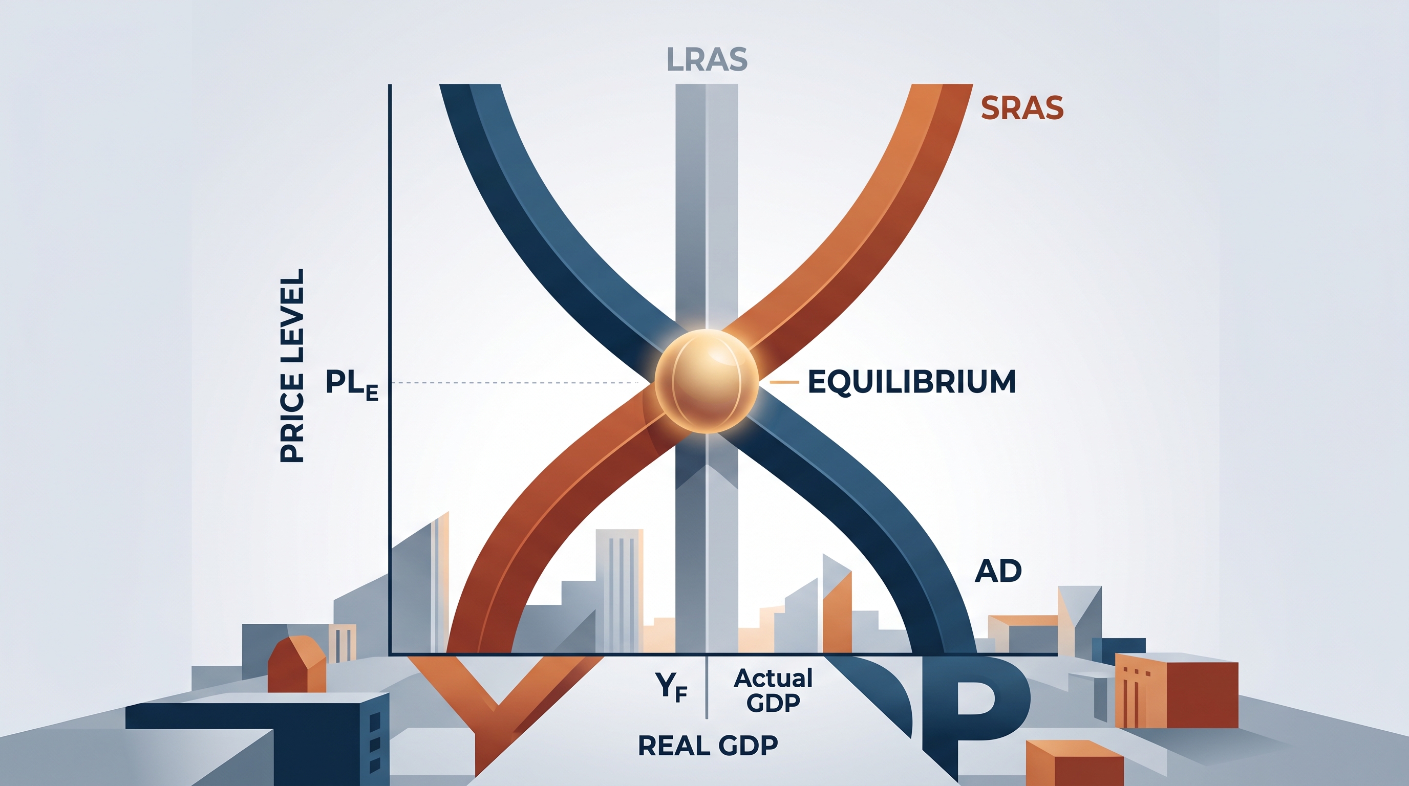
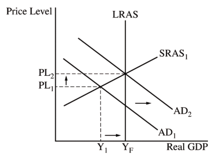

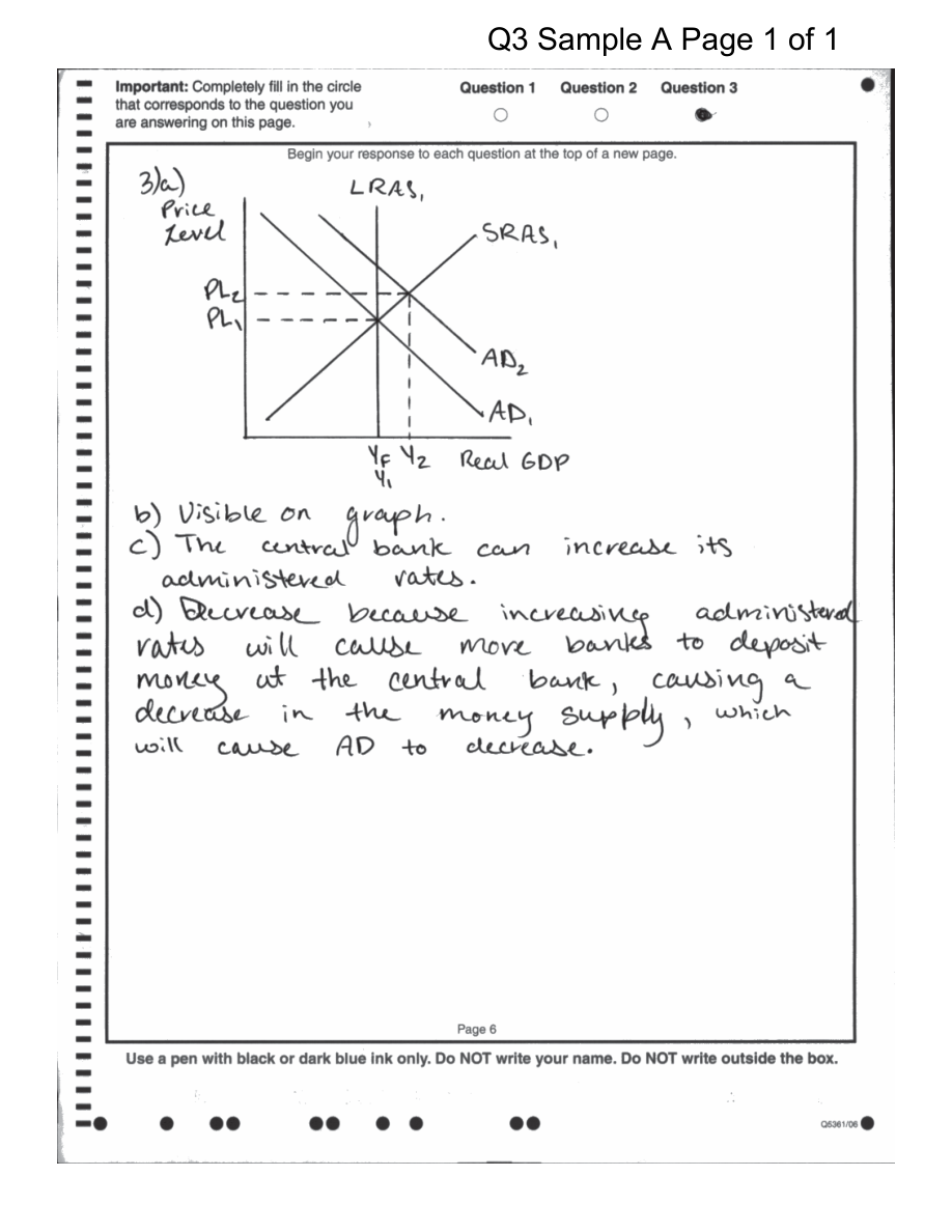
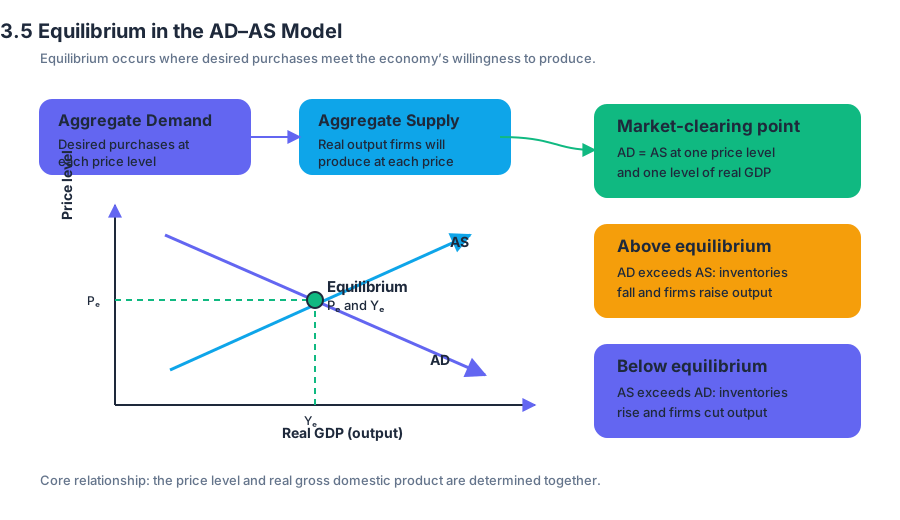
3.6 Changes in the AD–AS Model in the Short Run
Key concepts: Short-run changes in the AD–AS model · Effects of macroeconomic changes on output, price level, and employment · Business-cycle turning points: peaks and troughs · Actual output, potential output, and recessionary gaps · Short-run and long-run equilibrium · The short-run aggregate supply (SRAS) curve · Sticky wages and prices · Production costs and inflationary expectations as determinants of SRAS · The long-run aggregate supply (LRAS) curve · The Phillips curve and macroeconomic shocks
A recessionary gap exists when an economy’s actual output is below its potential output, so firms produce less and employ fewer workers than they would at full employment.
3.6 Changes in the AD–AS Model in the Short Run
A recessionary gap exists when an economy’s actual output is below its potential output, so firms produce less and employ fewer workers than they would at full employment. The AD–AS model makes this gap visible by comparing the short-run equilibrium output with the economy’s sustainable capacity.
The time horizons: short run versus long run
In the short run, some input prices—especially nominal wages—are sticky, meaning they do not adjust immediately when economic conditions change. Because firms’ costs are temporarily fixed, a change in the price level can change firms’ profit incentives and the quantity of output they supply.
In the long run, all wages and prices are flexible. Once input prices fully adjust, changes in the overall price level no longer change the economy’s real productive capacity. Potential output depends instead on resources, technology, productivity, and institutions.
Why SRAS slopes upward
The short-run aggregate supply (SRAS) curve shows the relationship between the price level and the quantity of goods and services supplied in an economy (MOD-2.C.1). It slopes upward because wages and other prices are sticky in the short run (MOD-2.C.2): if firms can sell output at higher prices while their input costs have not risen proportionally, production becomes more profitable.
A movement along SRAS is caused by a change in the price level. A shift of SRAS is caused by a change in production costs (MOD-2.C.3). For example, higher expected inflation may lead workers to negotiate higher nominal wages. Higher wages raise firms’ costs, shifting SRAS left; lower wages or lower inflationary expectations reduce costs, shifting SRAS right.
Named misconception — “Every change in output shifts SRAS.” A change in the price level causes movement along a given SRAS curve. A change in wages, resource prices, productivity, taxes on production, or inflationary expectations shifts the entire curve.
LRAS and the two kinds of equilibrium
The long-run aggregate supply (LRAS) curve is vertical at potential output, labeled $Y_F$. Its vertical shape shows that a long-run change in the price level does not change real output: once wages and prices adjust fully, the economy returns to its productive capacity.
Short-run equilibrium occurs where $AD$ intersects $SRAS$. Long-run equilibrium occurs where $AD$ intersects $LRAS$ at potential output, $Y_F$, with wages and prices fully adjusted. Thus, an economy can have a short-run equilibrium at an output level different from $Y_F$, but long-run equilibrium requires actual output to equal potential output.
If short-run equilibrium output is $Y_1$ and $Y_1<Y_F$, the economy has a recessionary gap. If output exceeds $Y_F$, it has an inflationary gap. The gap is measured horizontally on the AD–AS graph as the difference between actual output and potential output.
Shocks, output, prices, and employment
Macroeconomic changes affect output, the price level, and employment in both the short run and the long run, although the immediate effects can differ from the eventual capacity of the economy.
Suppose consumer confidence falls. Consumption decreases, so aggregate demand shifts left from $AD_1$ to $AD_2$. In the short run, the new intersection with SRAS produces lower real output and a lower price level. Firms need fewer workers, so employment falls and cyclical unemployment rises.
A positive demand shock works in the opposite direction: $AD$ shifts right, increasing both the short-run price level and real output. Higher output requires more labor, so employment rises and unemployment falls. This movement along SRAS illustrates the short-run inverse relationship between inflation and unemployment identified in MOD-2.D.1, without implying that the trade-off lasts permanently.
A supply shock has a different signature. If energy prices rise, firms face higher production costs and SRAS shifts left. The economy experiences a lower level of output and a higher price level at the same time—a combination often called stagflation. Because employment is tied to production, unemployment tends to rise as well.
Peaks, troughs, and output gaps
A business-cycle peak is the turning point at which an expansion ends and the economy begins contracting. A trough is the turning point at which a contraction ends and a new expansion begins.
On a time graph of actual output, a peak is the highest point before output turns downward, while a trough is the lowest point before output turns upward. A recessionary gap can occur during a contraction when actual output falls below potential output, even though potential output itself may continue growing.
Worked example: reading an AD–AS shock
An economy begins with $Y_1=950$ billion and potential output of $Y_F=1{,}000$ billion. The recessionary gap is
$$ Y_F-Y_1=1{,}000-950=$50\text{ billion}. $$
If a decline in investment shifts $AD$ left, the short-run result is lower real output, a lower price level, and higher cyclical unemployment. The graph should show $AD$ shifting left while $SRAS$ and vertical $LRAS$ remain in place; the new short-run equilibrium lies left of $Y_F$.
Graphing skill 3.C: “Create a correctly labeled graph or visual to represent an economic model or market.” For an AD–AS response, label the vertical axis Price Level, the horizontal axis Real Output or Real GDP, draw downward-sloping $AD$, upward-sloping $SRAS$, and vertical $LRAS$ when long-run capacity is relevant. Mark the initial and final equilibria and use arrows to show every curve shift.
Retrieval check
An economy’s $AD$ curve shifts right while SRAS remains unchanged. What happens in the short run to real output, the price level, employment, and unemployment? Answer: real output, the price level, and employment rise; unemployment falls. If the new output exceeds $Y_F$, the economy has an inflationary gap.
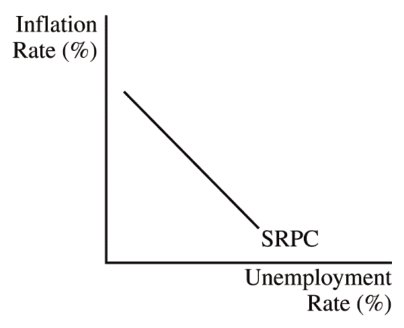
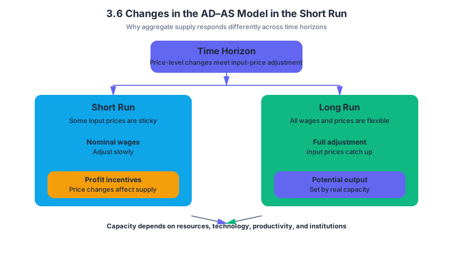
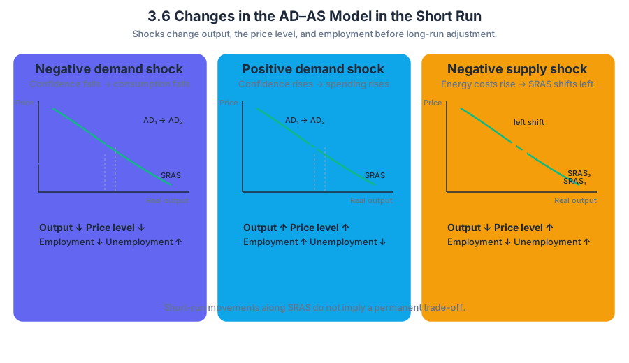
3.7 Long-Run Self-Adjustment
Key concepts: Long-run self-adjustment in the AD-AS model · Recessionary gaps and below-full-employment output · Downward pressure on nominal wages and input prices · Inflationary expectations and their effect on SRAS · Rightward shifts of the short-run aggregate supply (SRAS) curve · Restoration of full employment and potential output · Effects of shifts in aggregate demand on output and the price level · Using economic concepts and models to determine outcomes
A recessionary gap does not necessarily last forever: when real output falls below the economy’s full-employment level, persistent unemployment can gradually lower firms’ input costs and shift short-run aggregate supply rightward until potential output is restored.
3.7 Long-Run Self-Adjustment
A recessionary gap does not necessarily last forever: when real output falls below the economy’s full-employment level, persistent unemployment can gradually lower firms’ input costs and shift short-run aggregate supply rightward until potential output is restored.
Investigative question: If a fall in consumer spending shifts aggregate demand left, why might the economy eventually return to full employment without a new policy action—and why would the final price level be lower?
CED alignment: Enduring Understanding MOD-2; Learning Objective MOD-2.I; Essential Knowledge MOD-2.I.1 and MOD-2.I.2; Suggested Skill 3.A: Manipulation — Determine the outcome of an economic situation using economic concepts, principles, or models.
From an AD shock to a recessionary gap
Suppose households suddenly become cautious and reduce consumption. Because consumption is part of aggregate demand, the AD curve shifts left. In the short run, the economy moves to a new equilibrium with both a lower price level and lower real output.
A recessionary gap exists when actual real output is below the full-employment or potential-output level, written as $Y_F$. The economy is producing less than it could when its labor and other resources are employed at sustainable full-employment levels.
The crucial distinction is between the immediate result and the later adjustment:
| Stage | Output | Price level | Main mechanism |
|---|---|---|---|
| Initial equilibrium | $Y_F$ | $PL_1$ | Economy is at full employment |
| Short run after AD shifts left | Below $Y_F$ | Below $PL_1$ | Lower spending reduces production |
| Long run | Returns to $Y_F$ | Below $PL_1$ | Lower input costs shift SRAS right |
Why unemployment changes costs
In the recessionary gap, firms sell less and reduce production. They need fewer workers, so unemployment rises. If unemployment remains high, workers have less bargaining power and nominal wages—wages measured in current dollars—face downward pressure. Other input prices may also decline as firms reduce their demand for materials, energy, transportation, and rented capital.
Lower input prices reduce firms’ per-unit production costs. At every possible price level, firms can now profitably produce more output. Economically, this is an increase in SRAS, represented by a rightward shift of the short-run aggregate supply curve.
Inflationary expectations also matter
The adjustment is not limited to wages and physical inputs. Inflationary expectations are what households and firms anticipate about future inflation. If a prolonged recession causes people to expect lower inflation, workers may negotiate smaller wage increases and firms may set lower prices. Those expectations reduce cost pressures and can also shift SRAS rightward.
The process continues in stages: lower output creates unemployment; unemployment places downward pressure on nominal wages and other input prices; lower costs increase SRAS; and the new equilibrium produces more real output. The adjustment stops when output returns to $Y_F$.
The final price level is lower
Imagine that consumer spending first shifts $AD_1$ leftward. The economy lands at a short-run equilibrium below $Y_F$, creating a recessionary gap. As SRAS shifts right, the economy moves along the unchanged AD curve toward $Y_F$.
Because the new intersection occurs farther down the downward-sloping AD curve, the final equilibrium price level is less than the initial level $PL_1$. Output returns to full employment, but the price level does not return to its original value.
Key result: After long-run self-adjustment from a recessionary gap, real output returns to $Y_F$, while the final price level is below the initial price level $PL_1$.
This result depends on identifying the correct curve shift. The original decline in consumer spending shifts AD left. The later response to unemployment and falling costs shifts SRAS right. LRAS does not shift merely because the economy is in a recession; a shift in LRAS represents a change in full-employment output or economic growth, as specified by MOD-2.I.2.
Misconception check: “The recession fixes itself by shifting AD back”
Misconception: Students often draw AD shifting right during self-adjustment. That would mean aggregate demand has recovered, but self-adjustment describes a change in production costs and expectations. Therefore, the correct movement is a rightward shift of SRAS, not AD.
A second misconception is that returning to full employment means returning to the original price level. It does not. With AD unchanged, a rightward SRAS shift restores $Y_F$ at a lower price level than $PL_1$.
Skill 3.A in action
To apply 3.A: Manipulation, trace the complete causal chain rather than naming only the first effect:
$$ C \downarrow \Rightarrow AD \text{ shifts left} \Rightarrow Y \downarrow,\ PL \downarrow \Rightarrow u \uparrow \Rightarrow \text{nominal wages and input prices} \downarrow \Rightarrow SRAS \text{ shifts right} \Rightarrow Y \to Y_F,\ PL < PL_1 $$
Retrieval check: An economy is initially at $Y_F$. Consumer confidence falls, shifting AD left. In the long run, what curve shifts, what causes that shift, and how does the final price level compare with the original price level? The complete answer is: SRAS shifts right because high unemployment lowers nominal wages, input costs, and possibly inflationary expectations; output returns to $Y_F$, and the final price level is below the original $PL_1$.
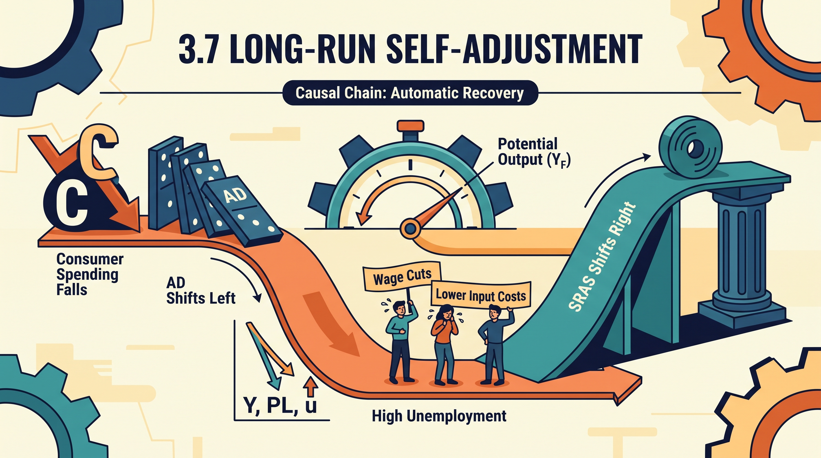
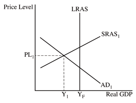
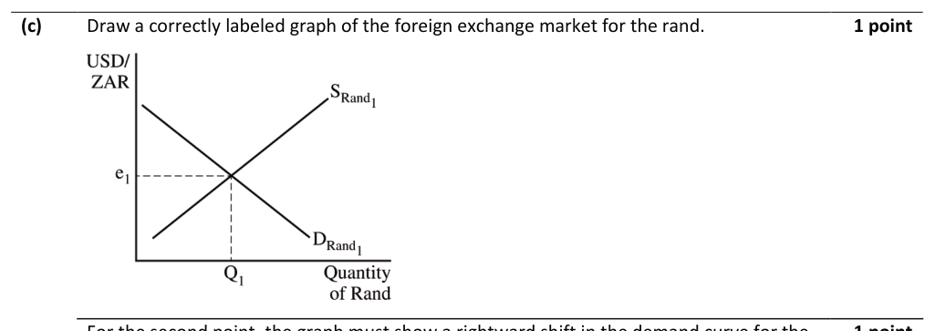
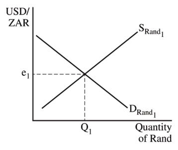
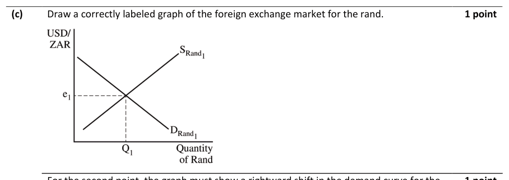
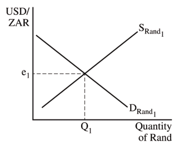
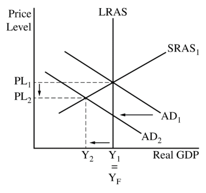
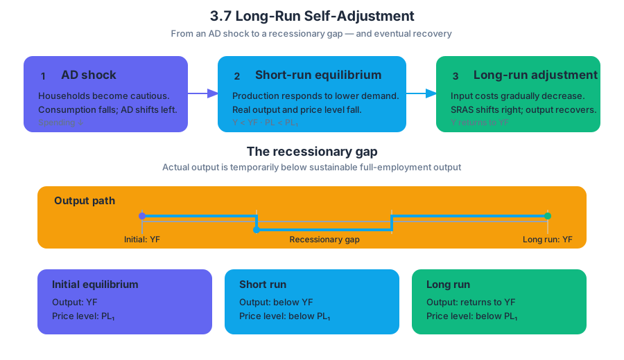
3.8 Fiscal Policy
Key concepts: Fiscal policy · Physical capital accumulation · Graphical analysis of policy changes
Fiscal policy is the government’s use of spending, taxation, and transfer payments to influence aggregate economic activity. The central policy question is not merely whether government action changes output, but whether its short-run benefit creates a long-run cost through higher interest rates, reduced…
3.8 Fiscal Policy
Fiscal policy is the government’s use of spending, taxation, and transfer payments to influence aggregate economic activity. The central policy question is not merely whether government action changes output, but whether its short-run benefit creates a long-run cost through higher interest rates, reduced investment, and slower growth.
Expansionary fiscal policy increases aggregate demand in the short run, but financing the policy can raise real interest rates and cause crowding out—a reduction in private investment caused by government borrowing.
The fiscal-policy transmission chain
The most common expansionary fiscal policies are:
- an increase in government purchases,
- a decrease in taxes, or
- an increase in transfer payments.
Each can increase household or business spending and shift aggregate demand, or AD, to the right. In the short run, real output rises, unemployment falls, and the price level increases.
The full causal chain is:
$$ G \uparrow \quad \text{or} \quad T \downarrow \quad \text{or} \quad TR \uparrow $$
$$ \Rightarrow \text{disposable income or planned spending} \uparrow $$
$$ \Rightarrow AD \text{ shifts right} $$
$$ \Rightarrow \text{real GDP} \uparrow,\ \text{price level} \uparrow,\ \text{cyclical unemployment} \downarrow $$
The effect is not necessarily equal to the initial policy change. For example, an increase in government purchases can generate additional rounds of consumption as recipients spend part of their new income. The final change in real GDP depends on the spending multiplier and on factors such as the marginal propensity to consume, taxes, imports, and crowding out.
Graphical analysis of a policy change
To explain a fiscal-policy change graphically, draw an accurately labeled AD–AS model:
- vertical axis: price level;
- horizontal axis: real GDP;
- downward-sloping $AD_1$;
- upward-sloping short-run aggregate supply, $SRAS$;
- initial equilibrium at $E_1$;
- rightward shift from $AD_1$ to $AD_2$;
- new equilibrium at $E_2$.
At $E_2$, the economy has a higher price level and greater real GDP than at $E_1$. A complete explanation must connect the graph to the policy: increased government purchases shift aggregate demand right; the new equilibrium raises real GDP and the price level in the short run.
A graph earns explanatory power only when every essential label is present. A curve’s direction alone is not enough: identify both axes, label the curves, mark the initial and final equilibria, and show the direction of the shift.
Why deficits can crowd out private investment
When government spending exceeds tax revenue, the government runs a budget deficit. To finance the deficit, it borrows in the loanable funds market. This increases the demand for loanable funds.
In the loanable funds model:
- vertical axis: real interest rate;
- horizontal axis: quantity of loanable funds;
- demand for loanable funds shifts right from $D_1$ to $D_2$;
- equilibrium real interest rate rises from $r_1$ to $r_2$;
- equilibrium quantity of loanable funds may rise.
The higher real interest rate makes borrowing more expensive for firms. Some firms cancel or delay purchases of factories, machinery, equipment, and technology. This decline in private investment is crowding out.
$$ \text{budget deficit} \uparrow \Rightarrow D_{\text{loanable funds}} \text{ shifts right} \Rightarrow r \uparrow \Rightarrow I \downarrow $$
The long-run cost: physical capital accumulation
Physical capital consists of productive assets such as machines, buildings, tools, and infrastructure. Physical capital accumulation occurs when an economy adds to its stock of these assets, allowing workers to produce more output per hour.
If crowding out reduces private investment, the economy accumulates physical capital at a lower rate. Over time, slower capital accumulation can reduce productivity growth and produce less economic growth than would otherwise occur.
$$ I \downarrow \Rightarrow \text{physical capital accumulation} \downarrow \Rightarrow \text{future productive capacity} \downarrow \Rightarrow \text{long-run economic growth} \downarrow $$
This creates an important distinction: expansionary fiscal policy may raise real GDP in the short run while reducing the growth of potential output in the long run if crowding out is substantial. The short-run demand gain and the long-run supply consequence must be analyzed separately.
Worked example: from stimulus to slower growth
Suppose an economy is below full employment. The government increases infrastructure spending, shifting $AD$ right. In the short run, real GDP increases from $Y_1$ to $Y_2$, the price level rises from $P_1$ to $P_2$, and cyclical unemployment falls.
The government finances the spending by issuing bonds. The resulting deficit shifts loanable-funds demand right, raising the real interest rate from $r_1$ to $r_2$. A firm that intended to borrow for new equipment now faces a higher financing cost and reduces its investment.
Therefore, the immediate policy effect is expansionary, but the later effect is a lower rate of physical capital accumulation. The economy may still grow, yet its future production possibilities expand more slowly.
Misconception check: “A deficit always reduces investment”
Misconception: Every government deficit causes complete crowding out. Correction: A deficit creates pressure for crowding out through higher demand for loanable funds, but the magnitude depends on the market. If substantial saving or capital inflows are available, the real interest rate may rise only slightly. If the economy has unused resources, the short-run increase in output may also offset some reduction in private investment.
Skill focus and retrieval check
This topic develops POL-3.C.3, explaining how fiscal policy affects economic outcomes; POL-3.C.4, explaining how fiscal policy may cause crowding out; and POL-3.B, analyzing policy effects through macroeconomic models. It also uses Skill Category 4: Graphing and Visuals, especially drawing correctly labeled graphs and explaining one or more changes using graphs.
Retrieval check: If expansionary fiscal policy is financed by government borrowing, what happens first in the loanable funds market, and how can that eventually produce a lower rate of physical capital accumulation?
Answer: Government borrowing shifts the demand for loanable funds right and raises the real interest rate. The higher rate reduces private investment, slowing the accumulation of physical capital and potentially reducing long-run economic growth.
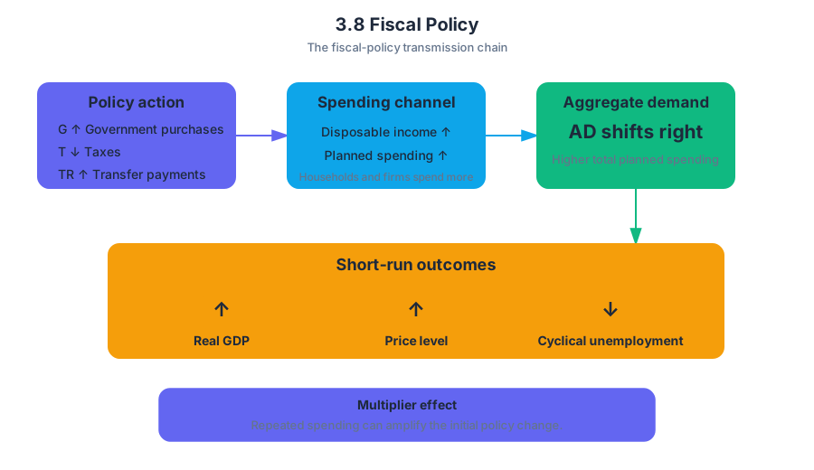
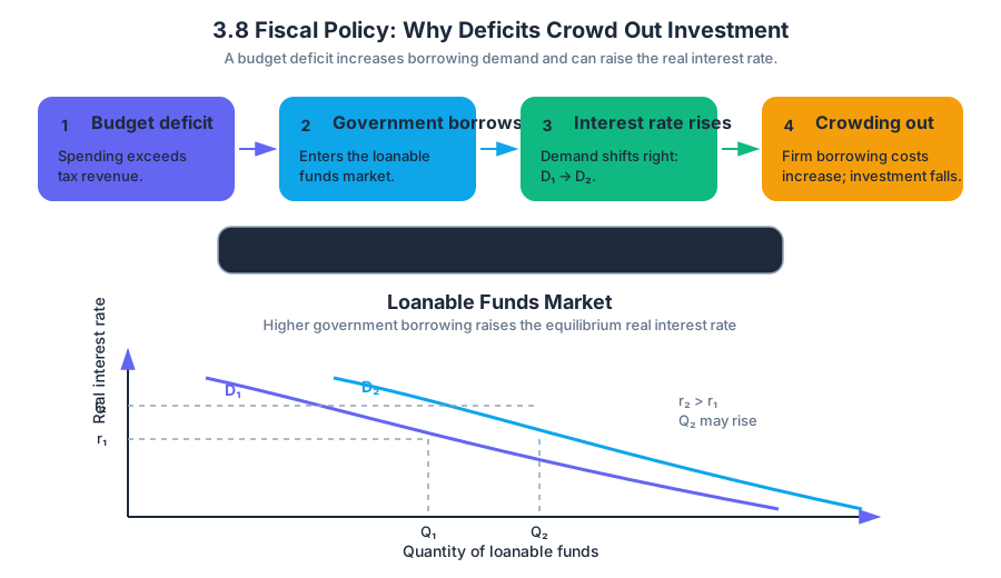
3.9 Automatic Stabilizers
Key concepts: Automatic stabilizers
When the economy slows, government transfer payments tend to rise while tax collections tend to fall—even if lawmakers pass no new policy. These built-in responses are automatic stabilizers: fiscal mechanisms that automatically soften expansions and contractions in the business cycle.
3.9 Automatic Stabilizers
When the economy slows, government transfer payments tend to rise while tax collections tend to fall—even if lawmakers pass no new policy. These built-in responses are automatic stabilizers: fiscal mechanisms that automatically soften expansions and contractions in the business cycle.
Learning Objective 3.9.A: Explain how automatic stabilizers affect the business cycle.
Automatic stabilizers work through the government’s effects on disposable income, the income households have available after taxes and including transfer payments. During a recession, disposable income falls less than it otherwise would, so consumption and aggregate demand decline by a smaller amount. During an expansion, the same mechanisms restrain excessive growth in disposable income and aggregate demand.
The automatic response
The key mechanism can be visualized as a two-sided shock absorber:
- Recession: Real GDP and employment fall $\rightarrow$ tax revenue falls and transfer payments rise $\rightarrow$ disposable income falls less $\rightarrow$ consumption falls less $\rightarrow$ aggregate demand is supported.
- Expansion: Real GDP and employment rise $\rightarrow$ tax revenue rises and transfer payments fall $\rightarrow$ disposable income rises less $\rightarrow$ consumption grows less rapidly $\rightarrow$ aggregate demand is restrained.
Common automatic stabilizers include a progressive income tax system, in which the tax rate rises as income rises, and transfer payment programs, such as unemployment benefits. These mechanisms do not eliminate the business cycle; they reduce the size of fluctuations in output, employment, and consumption.
Essential Knowledge 3.9.A.1: Automatic stabilizers are fiscal policy mechanisms that work automatically to reduce fluctuations in the business cycle.
Essential Knowledge 3.9.A.2: Automatic stabilizers include progressive income tax systems and transfer payments.
Worked example: cushioning a recession
Suppose a negative spending shock initially reduces aggregate demand by $$100$ billion. Assume the marginal propensity to consume is $0.80$, so the simple spending multiplier is
$$ \frac{1}{1-\text{MPC}}
\frac{1}{1-0.80}
$$
Without any stabilizing response, the eventual change in real GDP could be
$$ \Delta Y = 5(-$100\text{ billion})=-$500\text{ billion}. $$
Now suppose the recession causes tax payments to fall by $$20$ billion and transfer payments to rise by $$30$ billion. Household disposable income therefore receives a $$50$ billion cushion. If households spend $80%$ of that additional disposable income, the first-round increase in consumption is
$$ $50\text{ billion}\times 0.80=$40\text{ billion}. $$
That extra consumption creates further income for other households, which creates additional consumption. Using the simple multiplier for this illustrative support,
$$ \Delta Y_{\text{support}}
5($40\text{ billion})
$200\text{ billion}. $$
The economy still experiences a downturn, but the automatic stabilizers prevent the initial decline from passing through the entire repeated-spending process without interruption. On an aggregate demand–aggregate supply diagram, the result is a smaller leftward movement of aggregate demand than would occur without the stabilizers.
Automatic versus discretionary fiscal policy
Discretionary fiscal policy requires an intentional change in government spending, taxes, or transfer payments. Automatic stabilizers require no new legislative decision: tax collections and transfer payments change as income and employment change.
| Feature | Automatic stabilizers | Discretionary fiscal policy |
|---|---|---|
| Trigger | Changes in income or employment | Deliberate government action |
| Timing | Begins automatically | Requires policy design and implementation |
| Examples | Progressive taxes, unemployment benefits | A new infrastructure program or tax law |
| Main effect | Moderates fluctuations | Intentionally changes aggregate demand |
Automatic stabilizers are especially valuable because discretionary policy can face recognition, legislative, and implementation lags. However, they also create larger government budget deficits during recessions and larger surpluses, or smaller deficits, during expansions. The budget balance changes as part of the stabilizing process; that change is not itself evidence that policymakers have adopted a new discretionary policy.
Misconception check: “A recession automatically causes expansionary fiscal policy”
Correction: A recession automatically produces expansionary effects through the budget system, not necessarily a new expansionary law. Falling tax revenue and rising transfers support aggregate demand, but government officials may not have changed tax rates, spending laws, or eligibility rules.
A second common error is to say that automatic stabilizers increase aggregate demand during every recession. More precisely, they make aggregate demand higher than it would have been without them. Aggregate demand may still decrease overall; the decline is simply smaller.
AP skills and reasoning processes
Automatic stabilizers are commonly assessed through the official skill categories Skill Category 1: Principles and Models, Skill Category 2: Interpretation, Skill Category 3: Manipulation, and Skill Category 4: Graphing and Visuals.
- 1.B — Explain given economic outcomes: connect a recession to lower tax revenue, higher transfers, stronger disposable income, and a smaller decline in consumption.
- 2.B — Explain economic variables: distinguish changes in real GDP, disposable income, consumption, tax revenue, and transfer payments.
- 2.C — Interpret visual representations: read an AD–AS graph and identify the smaller change in equilibrium real output.
- 3.A — Calculate rate, ratio, or percentage change: calculate changes in tax revenue, transfers, or disposable income when data are provided.
- 3.C — Calculate an economic variable: apply the spending multiplier to estimate the effect of a change in consumption or government support.
- 4.A — Draw a correctly labeled graph: label the vertical axis as Price Level, the horizontal axis as Real GDP or real output, and show the appropriate AD shift and equilibrium changes.
Retrieval check
If real GDP falls and unemployment rises, what happens automatically to tax revenue and transfer payments, and why does that reduce the size of the recessionary decline in consumption? A complete answer should state: tax revenue falls, transfer payments rise, disposable income falls less, and consumption—and therefore aggregate demand—falls less than it otherwise would.
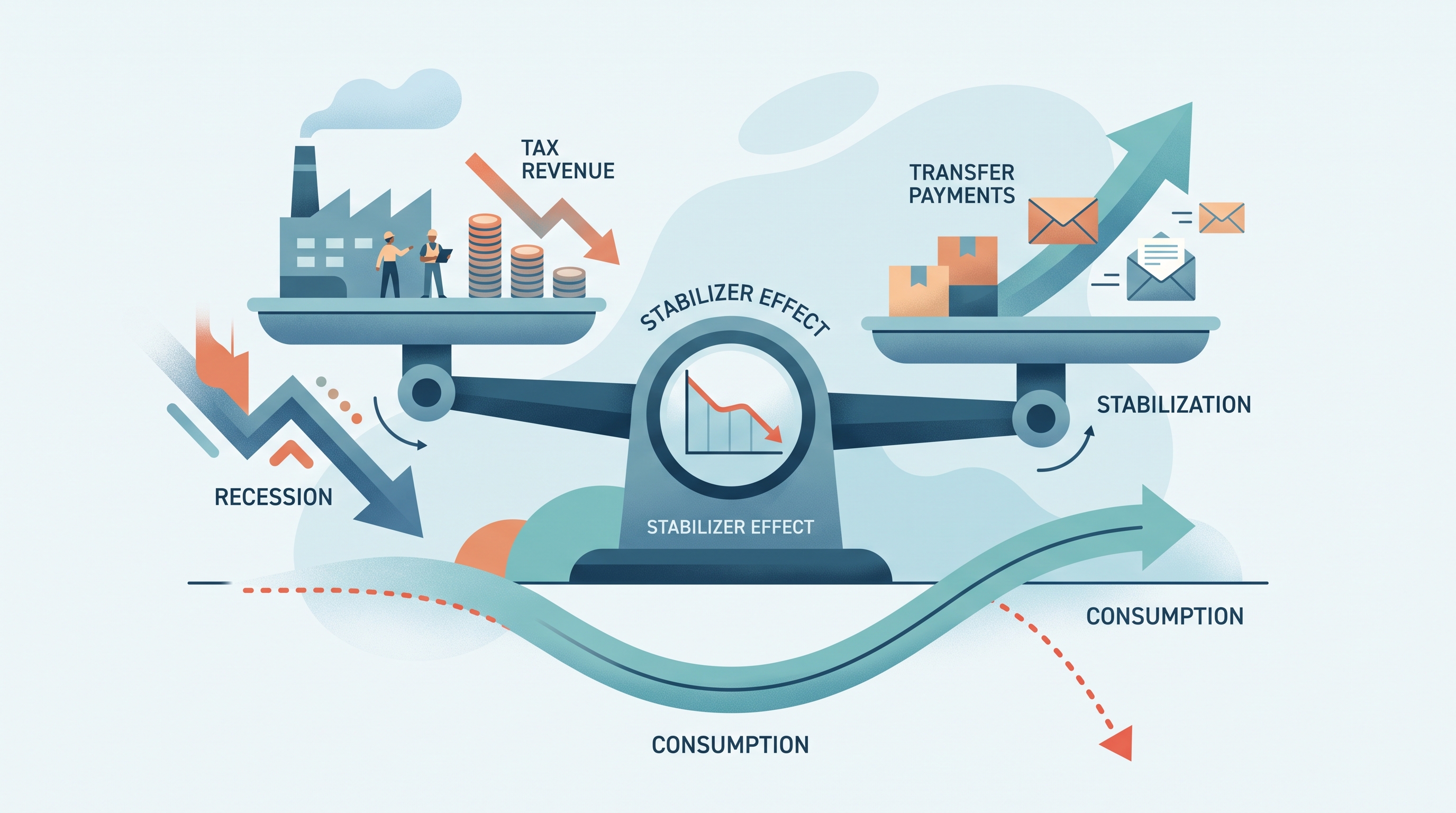
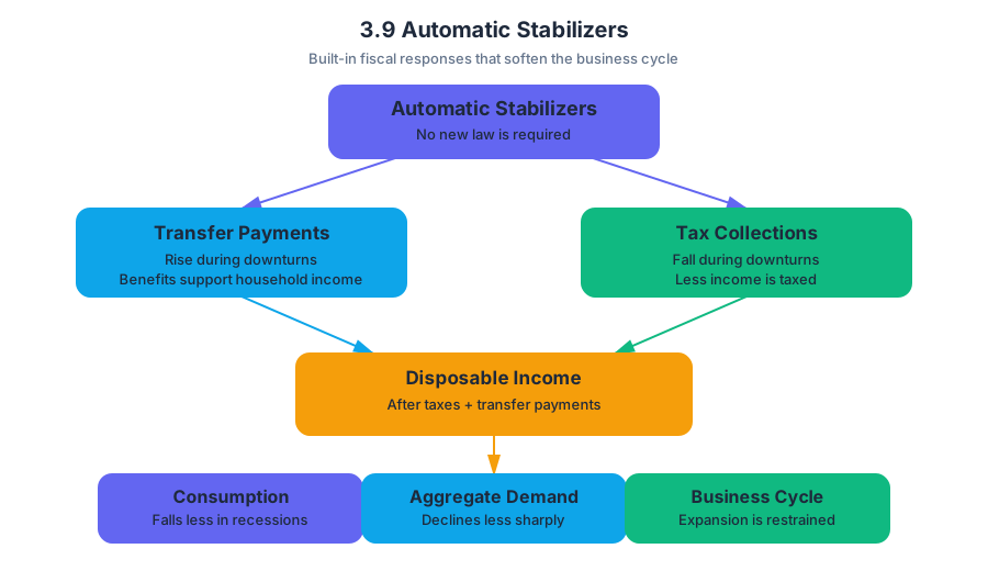
4.1 Financial Assets
Key concepts: Financial assets · Liquidity · Money · Cash · Demand deposits
A financial asset is valuable partly because of how quickly it can be used, sold, or exchanged without losing much value. That property is liquidity—and among the financial assets people hold, cash and demand deposits are the most liquid forms of money.
4.1 Financial Assets
A financial asset is valuable partly because of how quickly it can be used, sold, or exchanged without losing much value. That property is liquidity—and among the financial assets people hold, cash and demand deposits are the most liquid forms of money.
The three attributes of a financial asset
The CED identifies three principal attributes associated with financial assets, including money: liquidity, rate of return, and risk. These attributes help explain why people may choose to hold one asset instead of another.
Liquidity is the ease with which an asset can be converted into a means of payment, with little or no loss in value.
A dollar bill is immediately usable at a store. A house may be valuable, but converting it into spending power usually requires finding a buyer, negotiating a price, and completing a transaction. The house is therefore much less liquid than cash.
| Financial asset or form of money | How quickly it can be used for payment | Relative liquidity |
|---|---|---|
| Cash | Immediately | Very high |
| Demand deposit | Immediately through payment, withdrawal, or transfer | Very high |
| Bond | Usually must be sold first | Lower |
| Stock | Usually must be sold first; market price can change | Lower |
The trade-off is that highly liquid assets may not provide the same rate of return as assets designed for investment. Bonds are interest-bearing assets, while stocks are equity, meaning they represent ownership claims. People can hold bonds or stocks in place of the most liquid forms of money, but they generally must sell those assets before using the proceeds for ordinary purchases. This extra step makes them less liquid.
Money, cash, and demand deposits
Money is an asset accepted as payment for goods and services. In Topic 4.1, the important comparison is not simply whether an asset has value; it is whether the asset can function readily as a means of payment.
Cash—currency held by the public—is one of the most liquid forms of money. If a customer hands a seller a valid bill, the payment is complete immediately; no conversion, sale, or waiting period is required.
Demand deposits are funds held in checking accounts that can be accessed whenever the account holder demands them. A debit-card purchase, check, or electronic transfer allows the deposit to serve as money even though it is recorded in a bank account rather than held as physical currency.
The most liquid forms of money are cash and demand deposits (MEA-3.A.1).
A useful mental picture is a payment “ladder”:
$$ \text{Cash} ;\longleftrightarrow; \text{Demand deposits} ;\longrightarrow; \text{Immediate payment} $$
$$ \text{Bonds or stocks} ;\longrightarrow; \text{Sell the asset} ;\longrightarrow; \text{Receive funds} ;\longrightarrow; \text{Make payment} $$
The first path requires no asset sale. The second path does, so its usefulness for immediate purchases is lower.
Worked contextual example
Imagine that Maya receives $1,000 and must decide where to hold it for one month. She keeps $200 as cash, places $500 in a checking account, buys a bond with $200, and buys stock with $100.
If Maya needs to pay a $75 bill today, she can use either the cash or the demand deposit. Both are highly liquid. If she instead needs to use the bond or stock, she must sell the asset first, and the amount received may differ from the amount originally invested because market prices can change.
This example shows why liquidity is an attribute rather than a synonym for value. The stock may rise substantially in value, but that does not make it as immediately usable for payment as cash or a demand deposit.
Misconception check: “Anything valuable is money”
Misconception: A bond or stock is money because it can eventually be exchanged for money.
Correction: An asset’s ability to be sold is not the same as its ability to function directly as a means of payment. Cash and demand deposits are the most liquid forms of money; bonds and stocks are financial assets that people may hold instead (MEA-3.A.2).
AP reasoning in this topic
This topic develops MEA-3.A, especially MEA-3.A.a, which asks students to define the principal attributes—liquidity, rate of return, and risk—associated with various classes of financial assets, including money.
The relevant AP skill is Skill Category 1: Principles and Models, because students must apply the principle of liquidity to classify assets and predict which holdings are most convenient for immediate transactions. It also uses Skill Category 2: Interpretation when a prompt presents a list of assets, account types, or a financial decision and asks students to identify the most liquid option.
Retrieval check
A person owns $400 in currency, $600 in a checking account, $1,000 in a corporate bond, and $500 in stock. Which holdings are the most liquid forms of money, and why?
Answer: The $400 in currency and the $600 demand deposit are the most liquid forms of money because they can be used immediately for payment. The bond and stock must generally be sold before their value can be used for purchases.

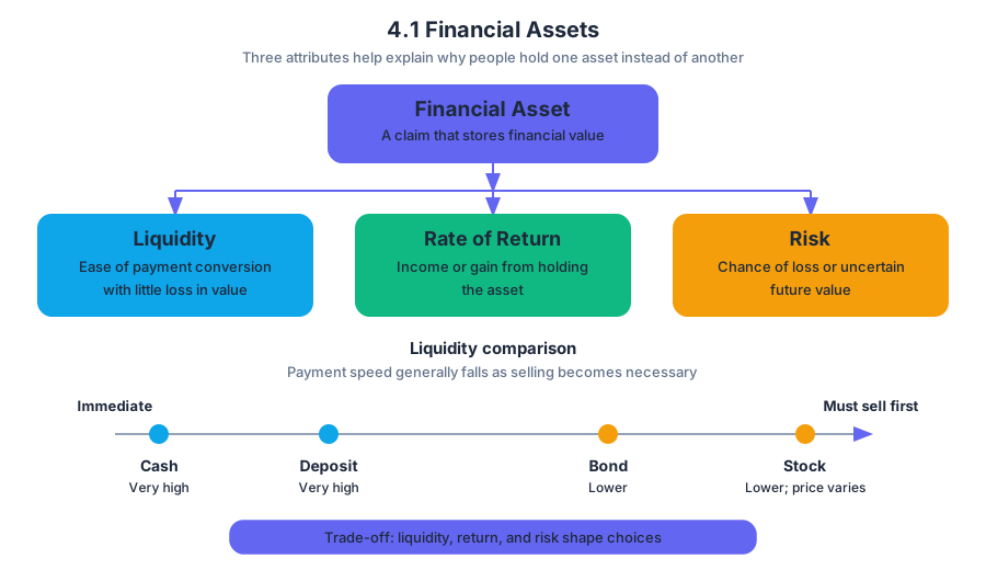
4.2 Nominal versus Real Interest Rates
Key concepts: Nominal interest rate · Real interest rate · Expected inflation · Actual inflation · Relationship between nominal and real interest rates · Lenders and borrowers · Inflation adjustment · Central bank influence on nominal interest rates · Interest rates as the price of money
An interest rate is the price of money: it tells a borrower what must be paid to use someone else’s money and tells a lender what return is earned for postponing consumption.
4.2 Nominal versus Real Interest Rates
An interest rate is the price of money: it tells a borrower what must be paid to use someone else’s money and tells a lender what return is earned for postponing consumption. The crucial question is whether that price is measured in ordinary dollars or adjusted for the changing purchasing power of those dollars.
Two interest rates, two perspectives
A nominal interest rate is the interest rate paid on a loan without adjustment for inflation. If a bank advertises a mortgage at $7%$, that $7%$ is nominal: it describes the dollar amount owed, not how much purchasing power the lender ultimately gains or the borrower ultimately sacrifices.
A real interest rate is the inflation-adjusted cost of borrowing or return to lending. It answers the economically meaningful question: After prices change, how much purchasing power has transferred from the borrower to the lender?
The distinction matters because a dollar received in the future may buy less than a dollar today. Inflation acts like a hidden adjustment to the loan: the nominal rate is written into the contract, while the real rate reveals the loan’s purchasing-power effect.
The expected-rate relationship
Before a loan is made, lenders and borrowers cannot know the exact future inflation rate. They therefore use expected inflation, the inflation rate they anticipate over the life of the loan, when negotiating the nominal interest rate.
MEA-3.B.2: Lenders and borrowers establish nominal interest rates as the sum of their expected real interest rate and expected inflation.
The relationship is:
$$ \text{Nominal interest rate}=\text{Expected real interest rate}+\text{Expected inflation} $$
Using standard notation, where $i$ is the nominal interest rate, $r^e$ is the expected real interest rate, and $\pi^e$ is expected inflation:
$$ i=r^e+\pi^e $$
Rearranging gives the expected real interest rate:
$$ r^e=i-\pi^e $$
For example, suppose a lender wants an expected purchasing-power return of $3%$ and expects inflation of $4%$. The nominal interest rate will be set at:
$$ i=3%+4%=7% $$
If expected inflation rises to $6%$ while the lender still requires an expected real return of $3%$, the nominal rate rises to:
$$ i=3%+6%=9% $$
The higher nominal rate does not necessarily mean the lender expects a higher real return. It may simply compensate for the expected loss in purchasing power.
Realized real interest: the hindsight calculation
After the loan period ends, economists can calculate the real interest rate in hindsight using actual inflation, the inflation rate that actually occurred rather than the rate people predicted.
MEA-3.B.3: A real interest rate can be calculated in hindsight by subtracting the actual inflation rate from the nominal interest rate.
The realized real interest rate is:
$$ r=i-\pi $$
Suppose a borrower signs a loan at a nominal rate of $7%$. If actual inflation turns out to be $5%$, the realized real interest rate is:
$$ r=7%-5%=2% $$
If actual inflation instead reaches $9%$, then:
$$ r=7%-9%=-2% $$
A negative real interest rate means the lender receives more dollars but loses purchasing power overall. The borrower repays the loan with dollars that are worth less than expected, making the borrowing cost negative in real terms.
Expected versus actual inflation
Keep the timing straight:
| When the calculation is made | Inflation measure | Formula |
|---|---|---|
| Before inflation occurs | Expected inflation, $\pi^e$ | $r^e=i-\pi^e$ |
| After inflation occurs | Actual inflation, $\pi$ | $r=i-\pi$ |
Named misconception — using actual inflation when setting the loan rate: A nominal interest rate is established using expected inflation, not inflation that has not yet occurred. Actual inflation is used later to calculate the realized real rate.
Named misconception — “nominal” means unimportant: Nominal rates determine the actual number of dollars paid or received. They are not economically sufficient by themselves because inflation determines what those dollars can purchase.
Lenders, borrowers, and central-bank influence
Lenders prefer a higher real return; borrowers prefer a lower real cost. Their agreement over the expected real return and expected inflation produces the nominal rate. If either expectation changes, the nominal rate can change even before any loan is signed.
The central bank does not directly set the economy-wide nominal interest rate. Instead, it influences nominal rates by changing its administered interest rates, such as the rates governing balances held by commercial banks. Those policy changes affect market interest rates, borrowing, lending, and interest-sensitive spending.
This distinction is especially important when analyzing monetary policy: a central bank’s higher administered rate can raise nominal market rates, while the effect on real rates depends partly on what happens to expected inflation.
AP skill connection: Principles and Models [1.A]
The suggested AP skill is Principles and Models [1.A]: Describe economic concepts, principles, or models. A strong response defines both rates precisely, identifies whether inflation is expected or actual, and uses the correct causal relationship rather than merely stating a number.
MEA-3.B: Define the nominal and real interest rate; explain the relationship between changes in nominal interest rates, expected inflation, and real interest rates; and calculate the nominal and real interest rate.
Retrieval check: A loan carries a nominal interest rate of $8%$. Expected inflation is $3%$, but actual inflation is $6%$. What are the expected real interest rate and the realized real interest rate?
Answer: Before the loan period, the expected real rate is $8%-3%=5%$. In hindsight, the realized real rate is $8%-6%=2%$. The two answers differ because they use different inflation measures.
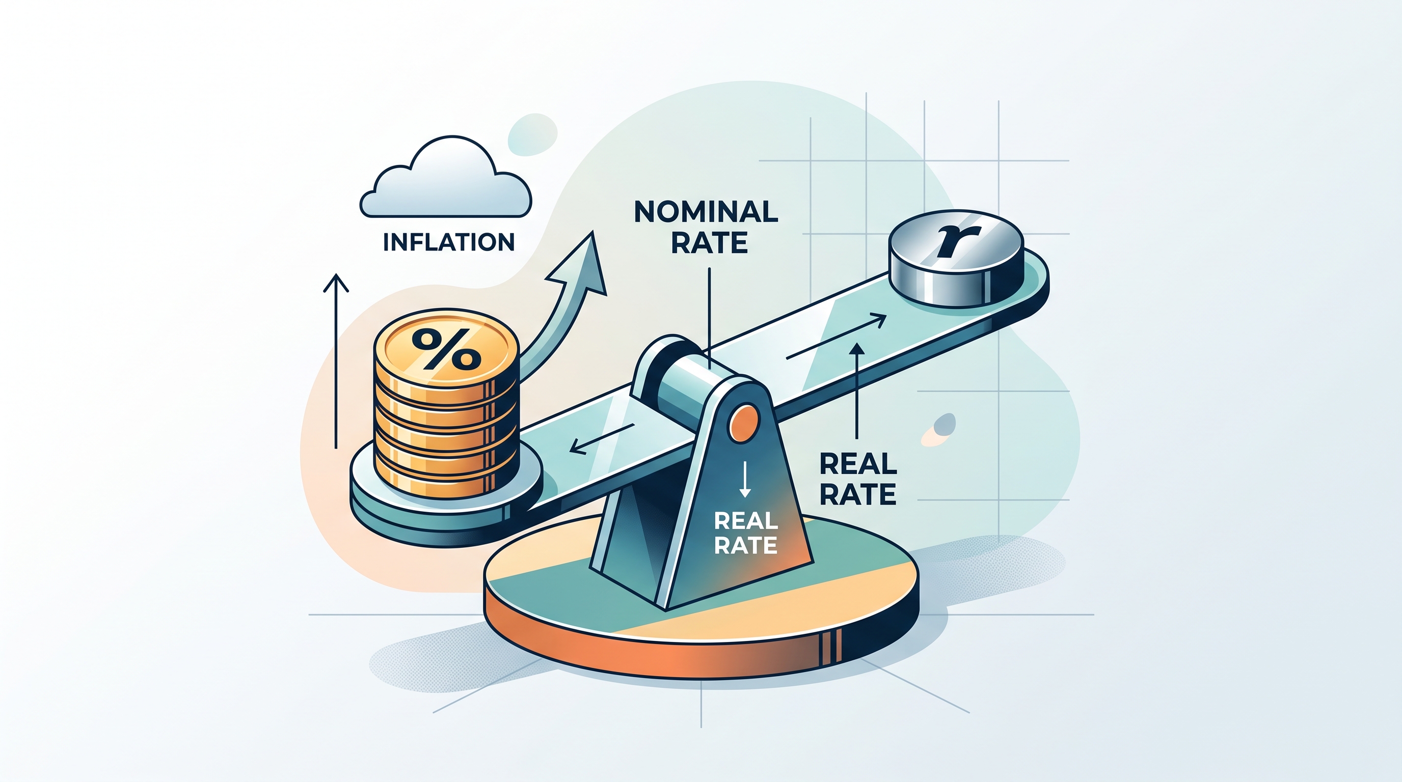
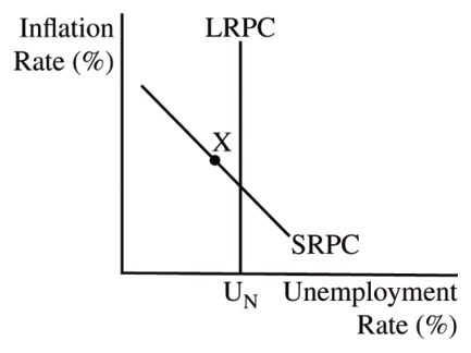
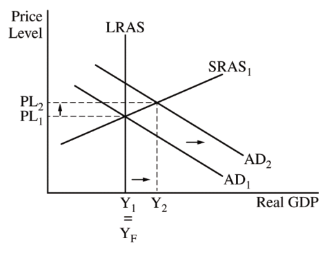
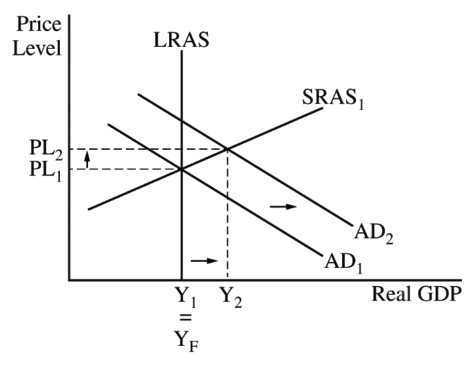
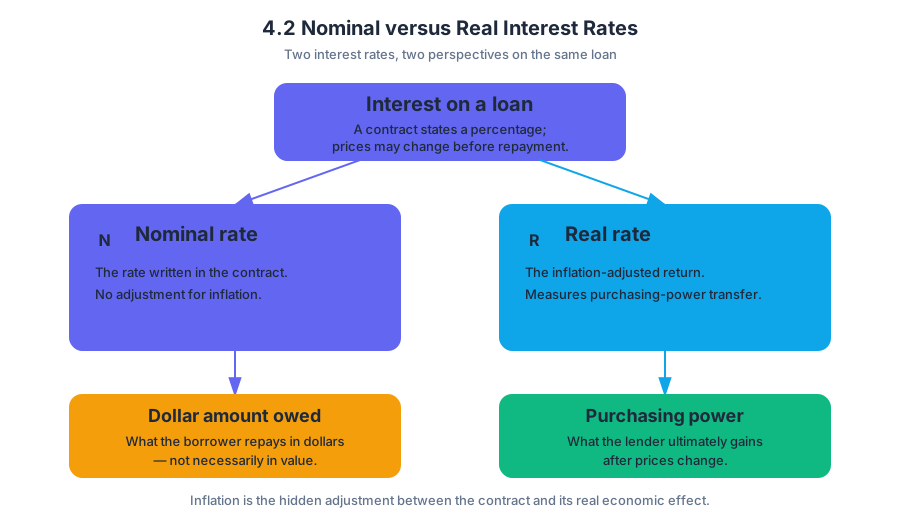
4.3 Definition, Measurement, and Functions of Money
Key concepts: Money as an asset generally accepted as payment · The three functions of money: medium of exchange, unit of account, and store of value · Liquidity and its relationship to money · Commodity money · Fiat money · The money supply · M1 · M2
Money is an asset that people generally accept as payment, allowing an economy to trade without requiring each buyer and seller to want exactly what the other offers.
4.3 Definition, Measurement, and Functions of Money
Money is an asset that people generally accept as payment, allowing an economy to trade without requiring each buyer and seller to want exactly what the other offers.
Imagine a bakery that wants flour, while the flour seller wants shoes rather than bread. Without money, the bakery must find someone who both sells flour and wants bread—a difficult double coincidence of wants. Money solves the problem by giving everyone a commonly accepted item to use between transactions.
What makes something money?
Money is an asset generally accepted as payment for goods and services and for the repayment of debts.
Money is not identical to wealth. Wealth includes houses, machinery, stocks, bonds, land, and other valuable assets. Money is one part of wealth, distinguished by its ability to function directly in transactions.
Money performs three connected functions:
- Medium of exchange: It facilitates transactions because sellers accept it in exchange for goods and services.
- Unit of account: It provides a common numerical system for measuring and comparing values.
- Store of value: It can be saved and used to purchase goods and services in the future.
A price such as $4.00 for a sandwich uses money as a unit of account: it lets consumers compare the sandwich with a $2.00 coffee or a $40.00 meal. When the customer hands over $4.00, money acts as a medium of exchange. If the customer keeps the remaining cash for next week, money acts as a store of value.
Retrieval check
A rare painting may be a valuable store of wealth, but it is usually a poor medium of exchange because most stores will not accept it at checkout. Which function of money is missing? Medium of exchange.
Liquidity: how quickly value can be spent
Liquidity is the ease with which an asset can be converted into a medium of exchange without losing value.
Currency is highly liquid: a $20 bill can be used immediately and normally retains its face value in the transaction. A house is much less liquid because selling it takes time, requires a buyer, and may involve a price reduction. A savings account is generally more liquid than a house but less immediately spendable than currency if transfers or withdrawals are restricted.
Liquidity explains why money is especially useful even when other assets may earn a higher return. Holding money makes transactions convenient, while holding less-liquid assets may require conversion before spending. The key question is not merely “Does this asset have value?” but “Can it become a means of payment quickly without losing value?”
Commodity money and fiat money
Commodity money has value partly because of the commodity itself. Gold, silver, or cigarettes used as money can have nonmonetary uses or value independent of their role in exchange.
Fiat money has value because the government declares it legal tender and because people accept it in payment. A modern dollar bill is not valuable because the paper can be used for another productive purpose; its purchasing power depends on legal recognition, public confidence, and acceptance throughout the economy.
| Type of money | Where its value comes from | Example |
|---|---|---|
| Commodity money | The underlying commodity itself, as well as its usefulness in exchange | Gold or cigarettes |
| Fiat money | Government designation as legal tender and public acceptance | Modern currency |
Misconception check — “Fiat” means worthless. Fiat money is not necessarily worthless or unstable. “Fiat” identifies the source of its value: legal status and acceptance rather than a valuable material contained in the money itself.
Measuring the money supply: M1 and M2
The money supply is the total quantity of money available in an economy, measured with monetary aggregates such as M1 and M2.
M1 focuses on assets used most directly for everyday payments. It includes:
- Currency in circulation
- Demand deposits
- Other checkable deposits
- Travelers’ checks
M2 includes everything in M1 plus assets that are slightly less liquid but can be converted into spendable funds relatively easily:
- Savings deposits
- Small time deposits
- Retail money market mutual fund shares
The relationship can be represented compactly as
$$ M2 = M1 + \text{savings deposits} + \text{small time deposits} + \text{retail money market mutual fund shares}. $$
For example, suppose an economy has $900$ billion in M1, $500$ billion in savings deposits, $100$ billion in small time deposits, and $50$ billion in retail money market mutual fund shares. Then
$$ M2 = 900 + 500 + 100 + 50 = 1{,}550\text{ billion dollars}. $$
The categories are aggregates, not separate piles of physical bills. Much of the money supply consists of account balances recorded electronically. Also, M2 is broader than M1, so an asset can be included in M2 without being as immediately spendable as currency.
AP skill connection: 1.B — Principles and Models
The suggested skill for Topic 4.3 is Skill Category 1: Principles and Models, 1.B: “Identify an economic concept, principle, or model illustrated by an example.” On an assessment, the task may present a situation rather than name the concept: a shopper pays with a debit card, a household holds savings, or a government requires a currency to be accepted for debts. The response must identify the relevant concept—medium of exchange, store of value, liquidity, fiat money, M1, or M2—and connect it to the evidence.
A reliable identification routine is:
- Ask whether the example concerns using, measuring, or saving money.
- If it concerns immediate spending, examine the asset’s liquidity.
- If it concerns the source of value, distinguish commodity money from fiat money.
- If it lists financial components, classify them under M1 or M2.
Final interpretation check: A household owns a certificate of deposit that cannot be withdrawn immediately without a penalty. Is it money in the same sense as currency? It is less liquid than currency and is included in M2 only when it meets the small-time-deposit definition; it is not part of M1.
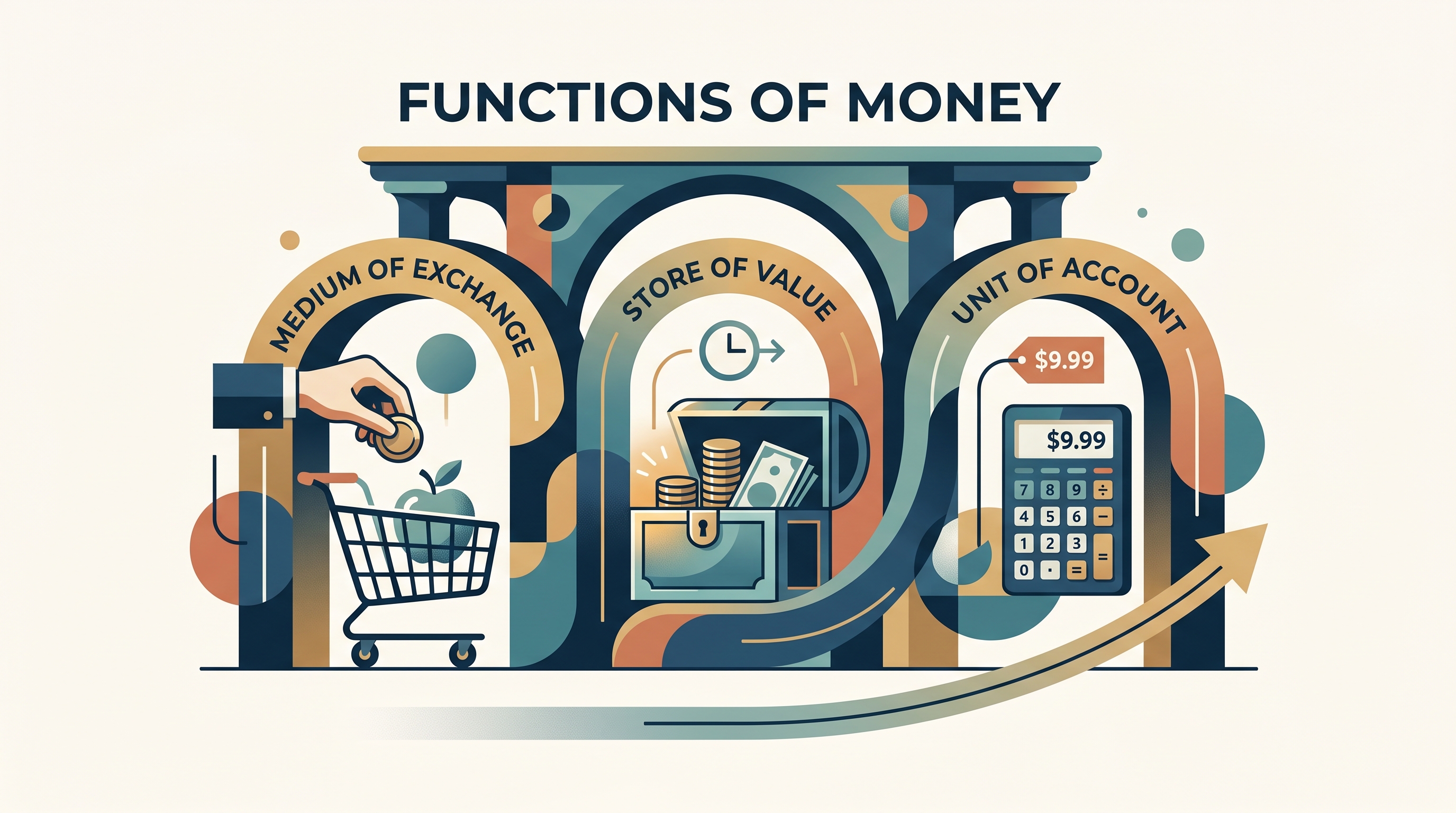
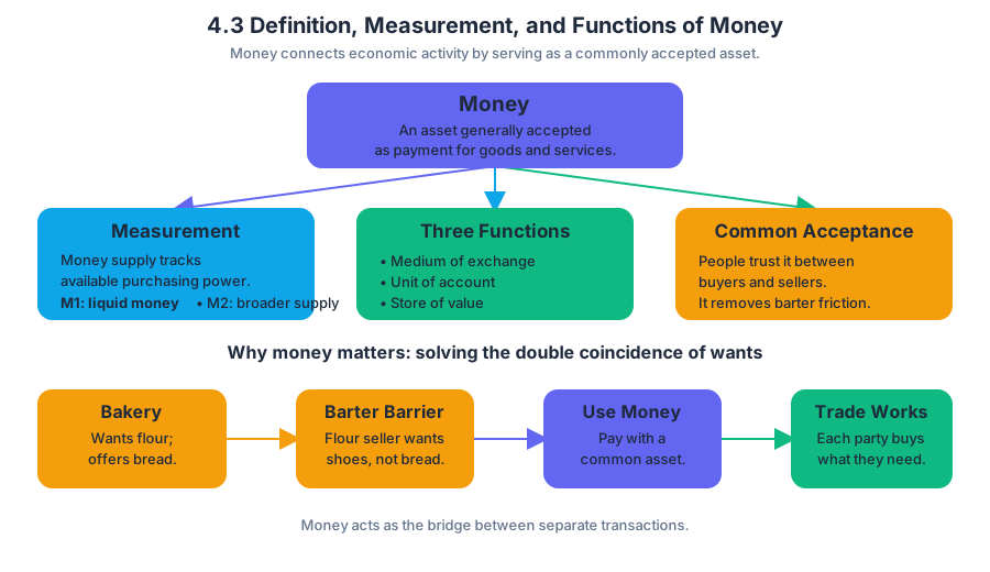
4.4 Banking and the Expansion of the Money Supply
Key concepts: Functions of money · Monetary base (M0 or MB) · Fractional-reserve banking · Money multiplier · Banking system and money-supply expansion · Bank reserves and currency holdings · Central-bank policy rate · Federal funds rate · Ample-reserves banking systems · Quantity theory of money
A bank can transform one deposit into a much larger volume of spendable deposits—not by printing currency, but by lending part of the reserves it holds.
4.4 Banking and the Expansion of the Money Supply
A bank can transform one deposit into a much larger volume of spendable deposits—not by printing currency, but by lending part of the reserves it holds. That process is fractional-reserve banking, and it explains how the banking system expands the money supply.
From money’s functions to bank-created deposits
A newly created bank deposit expands the money supply because the deposit can be used as a means of payment and held as a store of value. For example, when a bank credits a borrower’s checking account with a loan, the borrower can use that balance to purchase equipment even though no new physical currency has appeared.
The deposit also provides a unit of account: prices, debts, and loan balances can be recorded in the same monetary units. Thus, banking connects money’s functions to money creation: loans create deposits, and deposits make economic transactions possible.
Key idea: Banks do not create wealth simply by creating deposits. They create additional money-like purchasing power by recording deposits as liabilities while recording loans as assets.
The monetary base and bank balance sheets
The monetary base, also called $M0$ or $MB$, consists primarily of currency held by the public plus bank reserves held at the central bank. A bank’s balance sheet records what it owns as assets and what it owes as liabilities.
Under POL-2.A.1, depository institutions use balance sheets to track assets and liabilities. A customer’s checking-account deposit is the bank’s liability because the bank owes that amount to the depositor; the bank’s reserves and loans are assets.
The central distinction is that reserves are not identical to deposits. Reserves are claims held by banks at the central bank, while deposits are claims held by the public at banks. When a bank lends, reserves may support the transaction, but the borrower receives a deposit that can circulate through the economy.
Fractional-reserve banking
Under POL-2.A.2, banks operate through fractional-reserve banking: they hold only a fraction of deposits as reserves and lend or invest the remainder. The required reserve ratio, written as $r$, is the fraction of deposits a bank must hold as required reserves.
Reserves have two categories under POL-2.A.3:
- Required reserves: the minimum reserves associated with a bank’s deposits.
- Excess reserves: reserves held above the required minimum.
Excess reserves matter because they provide the immediate basis for additional lending and deposit creation, as identified in POL-2.A.4. A bank cannot safely expand loans indefinitely: it must maintain enough reserves to meet withdrawals, payments to other banks, and applicable requirements.
Worked example: one deposit, many deposits
Suppose a banking system receives an initial deposit of $1{,}000$ and the required reserve ratio is $0.10$. The first bank keeps $100$ as required reserves and lends $900$.
If the borrower spends the $900$ and the recipient deposits the payment in another bank, that second bank keeps $90$ and lends $810$. Repeated redepositing and relending produces the following idealized sequence:
$$ 1{,}000 + 900 + 810 + 729 + \cdots $$
The simple money multiplier is the ratio of the money supply to the monetary base, as specified in POL-2.A.5. Its maximum value is determined by the reciprocal of the required reserve ratio under POL-2.A.7:
$$ \text{Money multiplier}=\frac{1}{r} $$
Here,
$$ \frac{1}{0.10}=10 $$
so the maximum total deposit expansion from $1{,}000$ of new reserves is:
$$ \Delta \text{Deposits}=\frac{1}{r}\times \Delta \text{Reserves} =10\times 1{,}000 =10{,}000 $$
This is a maximum, not a guaranteed outcome. The calculation assumes every bank lends all excess reserves and that the public redeposits every dollar rather than holding currency.
Why actual expansion is smaller
Under POL-2.A.6 and POL-2.A.8, actual money-supply expansion depends on behavior throughout the banking system. The simple multiplier overstates expansion when banks hold excess reserves or when the public keeps more currency outside banks.
Misconception check — “A bank lends out the original deposit.” A bank does not hand the same deposit to the borrower and erase the depositor’s claim. It keeps the depositor’s account as a liability and creates a loan as an asset; the loan generally generates a new deposit in the borrower’s account. The banking system’s repeated process of deposits and loans expands the measured money supply.
Policy rates in an ample-reserves system
The central bank can influence nominal interest rates and the money supply through monetary policy. An interest rate is the price paid for borrowing money and the return received from saving.
The policy rate is the central bank’s administered target or operating rate—the rate it directly sets or closely controls through its policy tools. In the United States, the federal funds rate is the interest rate banks charge one another for overnight loans of reserves. The Federal Reserve influences this market rate by changing administered rates, especially the interest rate paid on reserves, which helps guide the federal funds rate toward the central bank’s desired level.
In a traditional limited-reserves system, changing the quantity of reserves can move the federal funds rate and affect lending conditions. In an ample-reserves system, banks already hold abundant reserves, so adding or removing reserves does not effectively change the nominal interest rate. Instead, the central bank primarily changes administered rates, including interest on reserves, to guide the federal funds rate and other market rates.
Exam distinction: In an ample-reserves system, expansionary policy means lowering administered rates—not necessarily increasing the quantity of reserves. Contractionary policy means raising administered rates.
Retrieval check
A bank receives $2{,}000$ in new reserves, and the required reserve ratio is $0.20$. The simple multiplier is $\frac{1}{0.20}=5$, so the maximum deposit expansion is $10{,}000$. If banks hold excess reserves or households hold currency, is the actual expansion larger, equal to, or smaller than $10{,}000$? Answer: smaller. In an ample-reserves system, would the central bank normally rely on a large change in reserves to alter the federal funds rate? Answer: no; it would adjust administered policy rates, such as interest on reserves.
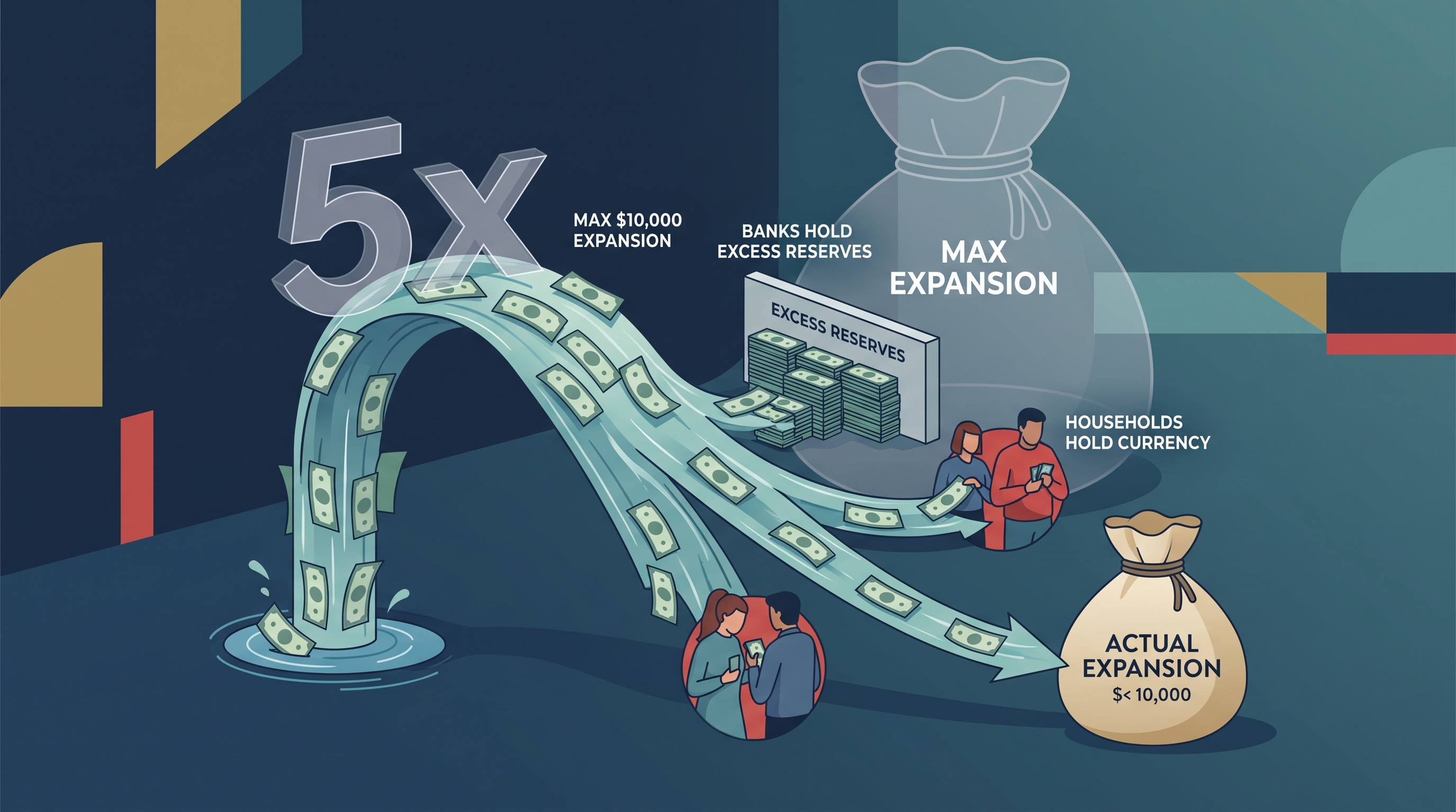
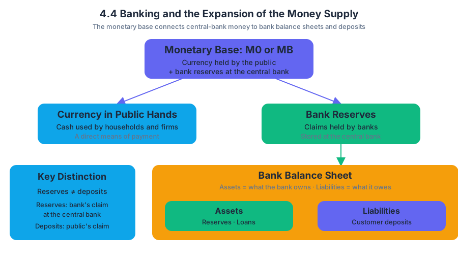
4.5 The Money Market
Key concepts: The money market · Money creation process · Money market versus reserve market · Interest rates and investment spending · Surpluses and shortages in a market · Transmission mechanisms linking policy actions to macroeconomic outcomes · Graphical analysis of markets · Fixed-interest-rate borrowers and inflation
The money market determines the economy’s nominal interest rate—the stated price paid to borrow money—through the interaction of the quantity of money people want to hold and the quantity available.
4.5 The Money Market
The money market determines the economy’s nominal interest rate—the stated price paid to borrow money—through the interaction of the quantity of money people want to hold and the quantity available. Its central question is simple: At what interest rate will money supplied equal money demanded?
CED traceability: Topic 4.5 The Money Market; Enduring Understanding MEA-3; Learning Objective MEA-3.D; Essential Knowledge MEA-3.D.1, MEA-3.D.2, and MEA-3.D.3. The topic emphasizes AP Skills 1.D: Describe the similarities, differences, and limitations of economic concepts, principles, or models, 3.A: Explain economic concepts, principles, or models, 3.B: Explain how a change in an economic situation affects a specific economic outcome, and 3.C: Calculate economic outcomes.
The money market model
Imagine households and businesses carrying a certain amount of cash or checking-account money because money is useful for purchases. Holding money, however, has an opportunity cost: funds kept as money do not earn the interest that could be earned in a bond or interest-bearing account. As the nominal interest rate rises, people generally hold less money and shift more wealth into interest-bearing assets.
Money demand is the quantity of money people choose to hold at each nominal interest rate. Money supply is the quantity of money available in the economy at each nominal interest rate.
In the standard money-market graph, the vertical axis is the nominal interest rate, $r$, and the horizontal axis is the quantity of money, $M$. The money-demand curve, $D_M$, slopes downward because a higher interest rate raises the opportunity cost of holding money. The money-supply curve, $S_M$, is vertical when the central bank fixes the quantity of money.
The intersection of $D_M$ and $S_M$ gives equilibrium: the equilibrium quantity of money and the equilibrium nominal interest rate. A change in the interest rate caused by movement along $D_M$ is not a shift in money demand. A shift occurs only when a determinant such as the price level changes.
Surpluses and shortages
A surplus of money occurs when the quantity of money supplied exceeds the quantity demanded at a particular interest rate. On the graph, this appears when the vertical distance from $S_M$ to $D_M$ indicates $M_S>M_D$. People attempt to reduce excess money holdings by purchasing bonds and other financial assets; bond prices rise, and the nominal interest rate falls toward equilibrium.
A shortage of money occurs when the quantity of money demanded exceeds the quantity supplied, or $M_D>M_S$. People try to obtain money by selling bonds or other assets. Bond prices fall, pushing the nominal interest rate upward until the quantity demanded equals the quantity supplied.
Worked example. Suppose the money supply is fixed at $500$ units. At a nominal interest rate of $8%$, households want to hold $650$ units. The market has a money shortage of
$$M_D-M_S=650-500=150\text{ units}.$$
People sell assets to acquire the missing $150$ units. The resulting decline in bond prices raises interest rates, reducing the quantity of money demanded. This is the complete adjustment mechanism—not merely “the interest rate increases.”
Money market versus reserve market
The money market analyzes the public’s demand for money and the economy’s total money supply. The reserve market analyzes commercial banks’ reserves—funds held at the central bank—and the interest rate used to influence banks’ lending behavior. These are related markets, but they are not interchangeable.
| Feature | Money market | Reserve market |
|---|---|---|
| Traded or analyzed quantity | Money held by the public | Bank reserves |
| Main demanders | Households and firms | Commercial banks |
| Vertical axis commonly used | Nominal interest rate | Policy or reserve-market interest rate |
| Typical policy connection | Money supply changes affect interest rates | Administered rates or reserve operations affect banks |
| Common graph error | Labeling reserves as money | Drawing the money-demand curve instead of reserve demand |
Misconception check — “The money market is the reserve market.” It is not. A question asking how households’ money holdings respond to interest rates requires a money-market graph. A question asking how a central bank changes the rate paid on reserves, or how banks respond to reserves, requires a reserve-market graph.
From money creation to macroeconomic outcomes
The “Case of the Gigantic $100,000 Bill” activity illustrates why one deposit can support a larger total money supply. When a bank receives a deposit, it keeps required reserves and lends the remainder. The borrower spends the loan, another person deposits those funds, and a second bank keeps part as reserves and lends the rest. Repeated redepositing and relending expands deposits through the banking system.
If the required reserve ratio is $rr$, the simple maximum-deposit multiplier is
$$\text{Money multiplier}=\frac{1}{rr}.$$
For example, with $rr=0.20$, an initial new reserve deposit of $$100{,}000$ could support a maximum change in deposits of
$$\Delta M=\frac{1}{0.20}\times $100{,}000=$500{,}000.$$
This is a theoretical maximum: the process is smaller if banks hold excess reserves or if households keep some loan proceeds as currency. The important chain is deposit $\rightarrow$ bank lending $\rightarrow$ spending and redepositing $\rightarrow$ additional deposits.
Interest rates, investment, and aggregate demand
A money-market change matters because interest rates influence interest-sensitive spending. Suppose the central bank reduces the money supply. With money demand initially unchanged, the fixed $S_M$ curve shifts left. At the original interest rate, a shortage of money appears, causing the nominal interest rate to rise.
The transmission mechanism must be stated in sequence:
$$ S_M\text{ shifts left} \rightarrow r\text{ rises} \rightarrow \text{borrowing becomes more expensive} \rightarrow I\text{ falls} \rightarrow AD\text{ shifts left} \rightarrow \text{price level and real output fall in the short run}. $$
Businesses cancel or postpone projects such as factory expansion, equipment purchases, and building construction when financing costs rise. Because investment spending is a component of aggregate demand, lower investment shifts $AD$ left; saying only “the price level falls” omits the mechanism required for a complete explanation.
Inflation and fixed-rate borrowers
Unexpected inflation changes the real burden of a fixed-interest-rate loan. If a borrower receives money when its purchasing power is relatively high and repays the same nominal amount after prices rise, the repayment money buys fewer goods and services.
Borrowers with fixed-interest-rate loans benefit from unexpected inflation because the money repaid is worth less than the money borrowed.
The lender receives the promised nominal payment, but its real value is lower than anticipated. This is distinct from a variable-rate loan, whose interest rate can adjust as inflation expectations or market conditions change.
Retrieval check
At an interest rate of $6%$, suppose $M_D=900$ and $M_S=700$. Is the money market experiencing a surplus or shortage, and what happens to the interest rate? Answer: There is a shortage of $200$ units because $M_D-M_S=200$. People sell assets to obtain money, bond prices fall, and the nominal interest rate rises. If the original disturbance was a fall in the money supply, identify it as a shift of $S_M$, not a movement along the curve.
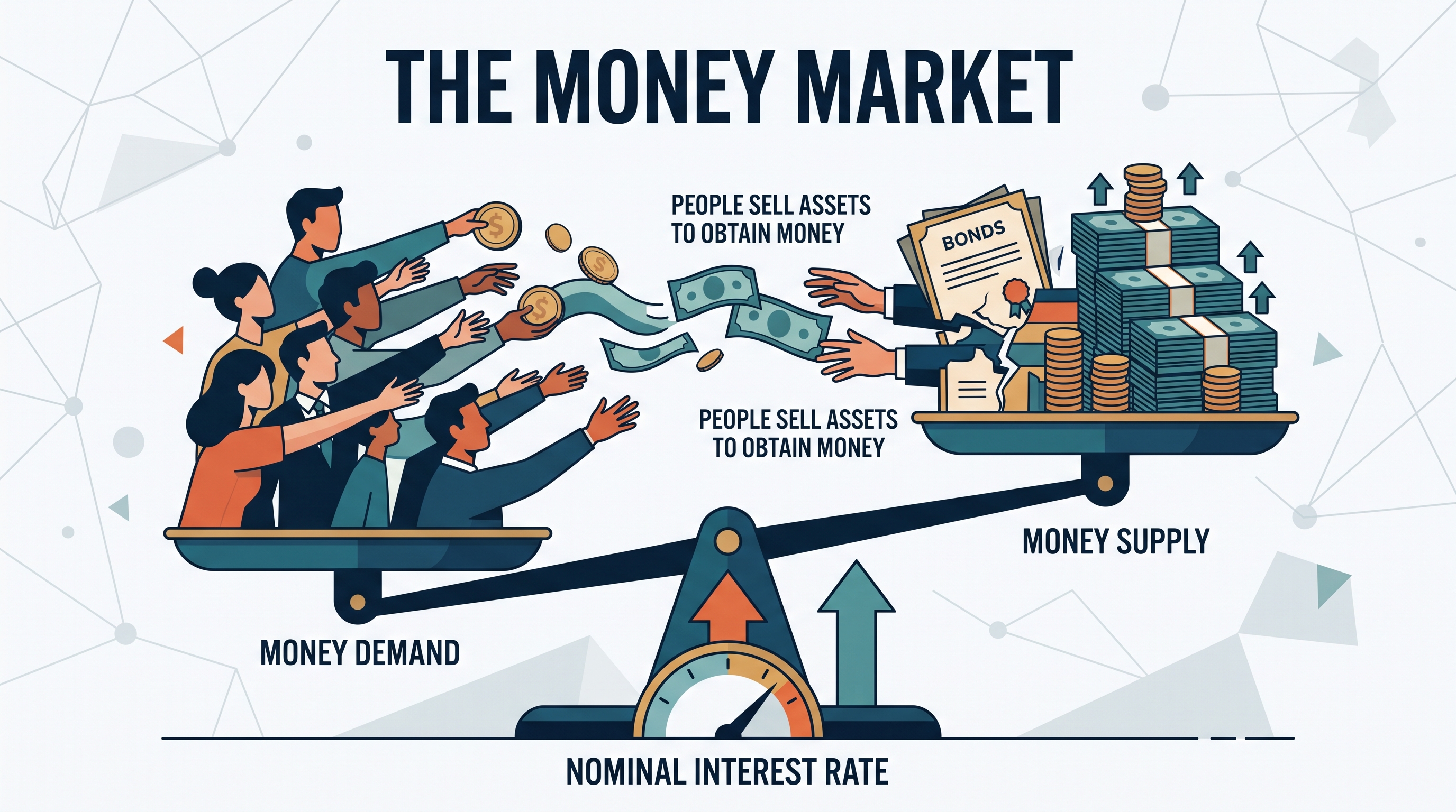
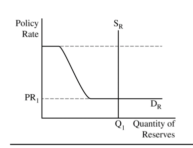
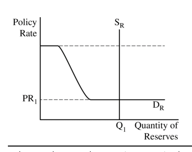
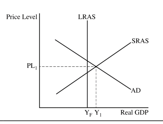
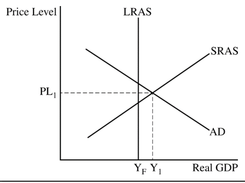
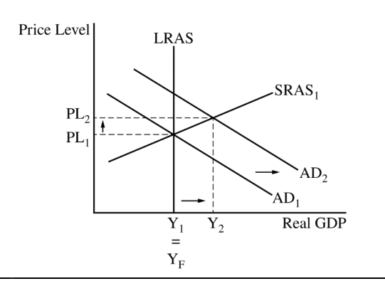
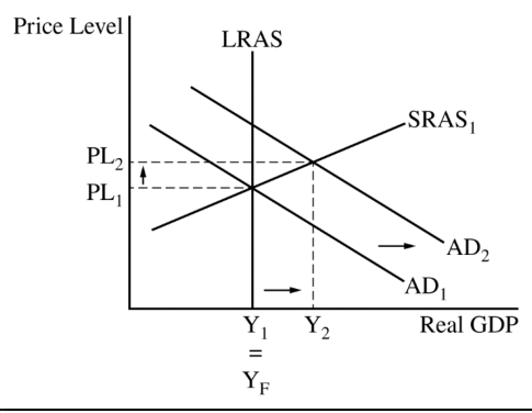
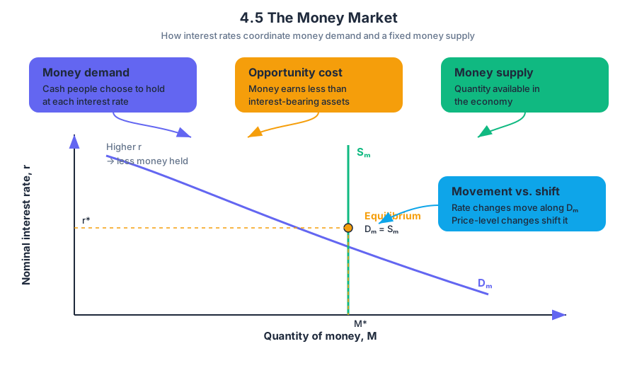
4.6 Monetary Policy
Key concepts: Monetary policy · Economic growth
When inflation rises too quickly or a recession leaves factories, workers, and machines idle, the central bank can influence spending by changing financial conditions. Monetary policy is the deliberate use of central-bank actions to affect the money supply, interest rates, aggregate demand, output, employment, and…
4.6 Monetary Policy
When inflation rises too quickly or a recession leaves factories, workers, and machines idle, the central bank can influence spending by changing financial conditions. Monetary policy is the deliberate use of central-bank actions to affect the money supply, interest rates, aggregate demand, output, employment, and the price level.
Monetary policy is conducted by the central bank—in the United States, the Federal Reserve—to pursue macroeconomic stability.
The policy transmission chain
The key is not the policy instrument by itself, but the chain of effects that follows. Using the money-market result that an increase in money supply lowers the nominal interest rate, expansionary policy can raise interest-sensitive spending and aggregate demand.
| Policy direction | Central-bank action | Interest rates | Spending and aggregate demand | Short-run macroeconomic result |
|---|---|---|---|---|
| Expansionary monetary policy | Increase the money supply or lower the policy interest rate | Decrease | Investment and interest-sensitive consumption increase; $AD$ shifts right | Real GDP and employment rise; the price level tends to rise |
| Contractionary monetary policy | Decrease the money supply or raise the policy interest rate | Increase | Investment and interest-sensitive consumption decrease; $AD$ shifts left | Inflationary pressure falls; real GDP and employment tend to decline |
For example, suppose an economy is operating below full employment. The Federal Reserve adopts expansionary monetary policy, which lowers the nominal interest rate. Firms find it cheaper to finance new equipment, households face lower borrowing costs for durable goods, investment rises, and aggregate demand shifts right. In the short run, real output increases from $Y_1$ toward potential output $Y_f$, while the price level rises from $PL_1$ to $PL_2$.
The reverse occurs when inflation is excessive. Contractionary monetary policy raises interest rates, discourages borrowing and investment, reduces aggregate demand, and slows increases in the price level. The trade-off is that weaker demand can reduce real GDP and employment in the short run.
Choosing the policy direction
A useful diagnostic is the output gap. A recessionary gap exists when equilibrium real GDP is below potential real GDP, $Y < Y_f$; expansionary monetary policy may help close it. An inflationary gap exists when equilibrium real GDP exceeds potential, $Y > Y_f$; contractionary monetary policy may reduce excess demand.
Policy effects are not instantaneous. Households and firms may take time to refinance loans, change purchases, or revise investment plans. The size of the response also depends on confidence, the sensitivity of investment to interest rates, and whether banks are willing to lend.
Monetary policy and economic growth
A short-run increase in real GDP is not automatically economic growth. Short-run recovery moves an economy closer to its existing productive capacity after a recession; long-run economic growth is a sustained increase in the economy’s productive capacity, shown by a rightward shift of the long-run aggregate supply curve, $LRAS$, or an increase in potential real GDP, $Y_f$.
Stable, appropriately managed monetary policy can support long-run growth indirectly. By reducing the severity of recessions, limiting damaging inflation, and helping maintain predictable financial conditions, it can encourage saving, investment, and productive planning. However, monetary policy alone cannot permanently increase the economy’s productive capacity: it cannot by itself create better technology, expand the labor force, improve human capital, or add physical capital.
Critical distinction: Expansionary monetary policy can raise actual output in the short run, but lasting growth requires an increase in potential output.
Misconception check
Misconception: “Lower interest rates always create economic growth.” Lower rates can increase aggregate demand and temporarily raise real GDP, but if the economy is already near capacity, the main effect may be a higher price level. Permanent growth requires productive-capacity changes, not merely stronger spending.
AP skill application
Topic 4.6 Monetary Policy develops Learning Objective 4.6.A: Explain how the Federal Reserve uses monetary policy to influence the economy and Learning Objective 4.6.B: Explain how monetary policy affects economic outcomes. Its essential knowledge includes 4.6.A.1, 4.6.A.2, 4.6.B.1, and 4.6.B.2: identify the policy direction, connect it to interest rates and financial conditions, trace the effect through spending and $AD$, and state the resulting changes in output, employment, and the price level.
The main assessed reasoning uses Skill Category 1: Principles and Models, especially 1.B Explain economic outcomes; Skill Category 2: Interpretation, especially 2.B Interpret economic models; Skill Category 3: Manipulation, especially 3.A Calculate economic quantities when numerical changes are supplied; and Skill Category 4: Graphing and Visuals, especially 4.A Draw models and graphs. On a graph, label the axes, identify $AD$, $SRAS$, and $LRAS$ when relevant, mark the initial and new equilibria, and show the direction of the shift.
Retrieval check
If the Federal Reserve raises interest rates while the economy is experiencing an inflationary gap, what happens to investment, aggregate demand, real GDP, and the price level in the short run? The expected chain is: investment decreases, $AD$ shifts left, real GDP decreases, and inflationary pressure falls.
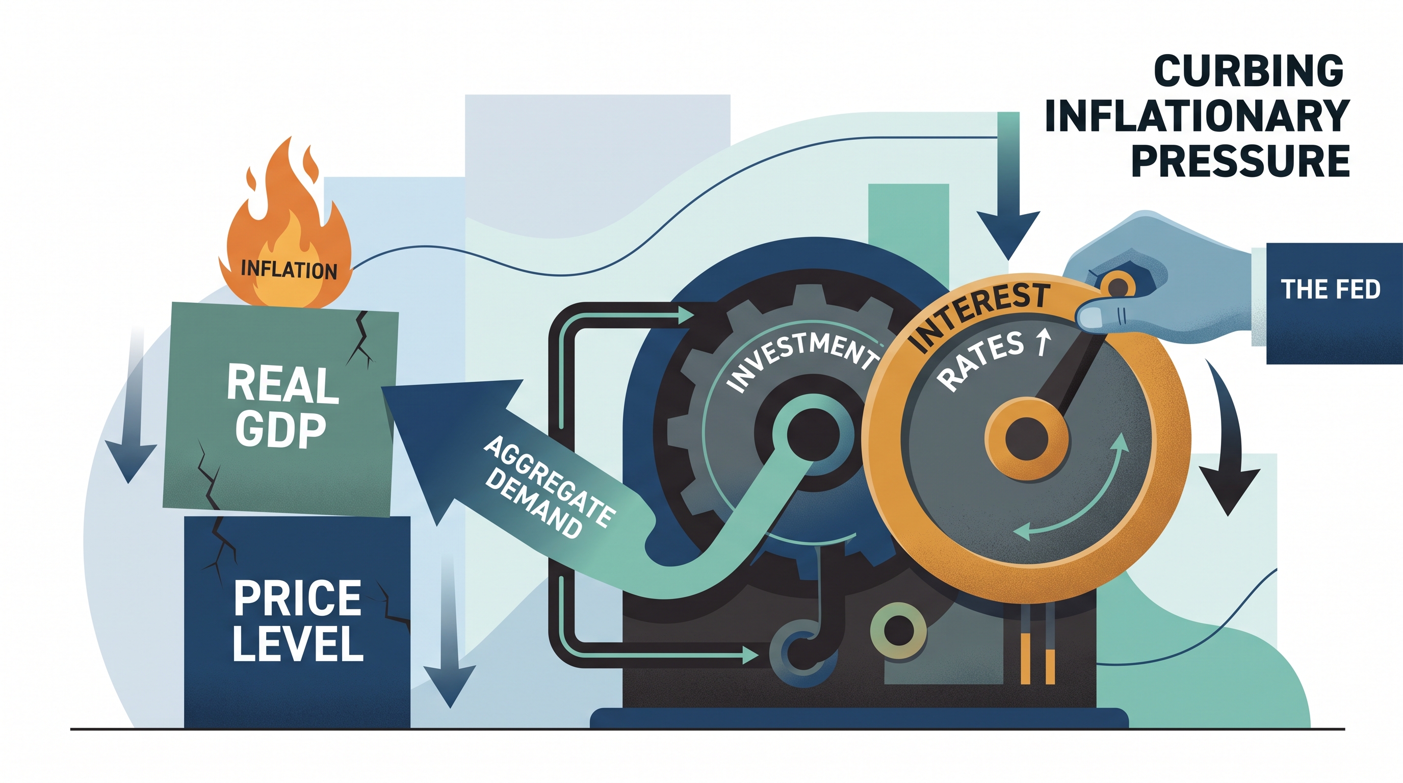
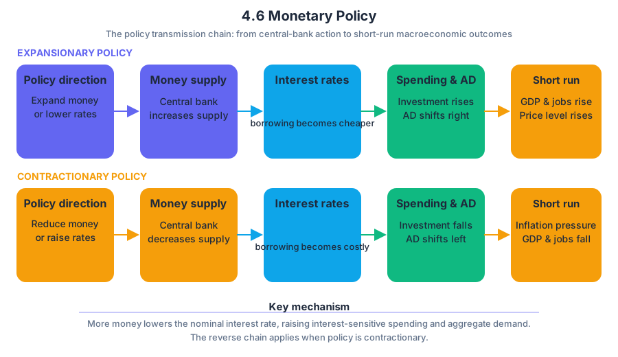
4.7 The Loanable Funds Market
Key concepts: Loanable funds market · Demand for loanable funds · Supply of loanable funds · Quantity of loanable funds demanded and supplied · National savings · Real interest rate · Market equilibrium · Surpluses and shortages in the loanable funds market · Government borrowing · Crowding out of private investment
The loanable funds market determines the equilibrium real interest rate—the interest rate adjusted for inflation—through the interaction of borrowers and savers. Borrowers demand funds to finance investment and government borrowing; savers supply funds by postponing current consumption.
4.7 The Loanable Funds Market
The loanable funds market determines the equilibrium real interest rate—the interest rate adjusted for inflation—through the interaction of borrowers and savers. Borrowers demand funds to finance investment and government borrowing; savers supply funds by postponing current consumption.
Enduring Understanding MKT-4: The interaction of borrowers, who demand loanable funds, and savers, who supply loanable funds, determines the equilibrium real interest rate.
The market’s two sides
The demand for loanable funds is the relationship between the real interest rate and the quantity of funds borrowers want at that rate. Because borrowing becomes more expensive when the real interest rate rises, the quantity of loanable funds demanded falls. This is an inverse relationship, so the demand curve slopes downward.
The supply of loanable funds is the relationship between the real interest rate and the quantity of funds savers are willing to lend at that rate. A higher real interest rate rewards saving more generously, so the quantity of loanable funds supplied rises. This positive relationship produces an upward-sloping supply curve.
In the standard graph, the vertical axis measures the real interest rate, $r$, and the horizontal axis measures the quantity of loanable funds, $Q_{LF}$. The downward-sloping demand curve is labeled $D_{LF}$, and the upward-sloping supply curve is labeled $S_{LF}$. At any particular real interest rate, read horizontally to determine the quantity demanded and the quantity supplied.
MKT-4.A.1: The loanable funds market describes the behavior of savers and borrowers.
MKT-4.A.2: The demand curve shows the inverse relationship between the real interest rate and the quantity demanded of loanable funds.
MKT-4.A.3: The supply curve shows the positive relationship between the real interest rate and the quantity supplied of loanable funds.
National savings supplies funds
National savings is a major source of loanable funds. In a closed economy, where there is no international trade or capital movement, national savings equals public savings plus private savings:
$$ S_{\text{national}} = S_{\text{private}} + S_{\text{public}} $$
Private saving is income not spent on consumption or taxes. Public saving is the government’s budget surplus, calculated as tax revenue minus government purchases and transfer payments. A budget deficit creates negative public saving, reducing national saving when private saving does not change.
In an open economy, domestic investment can be financed by national saving and funds entering from abroad. The required relationship is:
$$ I = S_{\text{national}} + \text{net capital inflow} $$
MKT-4.B.1: In a closed economy, national savings is the sum of public and private savings.
MKT-4.B.2: In an open economy, investment equals national savings plus net capital inflow.
Equilibrium, surplus, and shortage
Equilibrium occurs where the quantity of loanable funds demanded equals the quantity supplied. The intersection of $D_{LF}$ and $S_{LF}$ determines both the equilibrium real interest rate, $r_1$, and the equilibrium quantity of loanable funds, $Q_1$.
If the real interest rate is above $r_1$, lenders want to supply more funds than borrowers want to use. The market has a surplus of loanable funds, placing downward pressure on the real interest rate. If the real interest rate is below $r_1$, borrowers demand more funds than savers supply. The resulting shortage places upward pressure on the real interest rate.
MKT-4.C.1: Equilibrium occurs where the quantity of loanable funds demanded equals the quantity supplied.
MKT-4.D.1: Disequilibrium produces surpluses or shortages, and market forces move the real interest rate toward equilibrium.
Shifts: saving behavior and government borrowing
A change in the real interest rate causes a movement along an existing curve. A change in saving behavior changes the supply of loanable funds and shifts $S_{LF}$. For example, if households decide to save more at every real interest rate, $S_{LF}$ shifts right. The equilibrium real interest rate falls, while the equilibrium quantity of loanable funds rises.
The reverse also follows: a decrease in national saving shifts $S_{LF}$ left, raising the equilibrium real interest rate and lowering the equilibrium quantity of loans. This is why a fall in saving can make borrowing more expensive even when borrowers’ desire for funds has not changed.
Government borrowing increases the demand for loanable funds. Suppose the government finances a budget deficit by borrowing. The demand curve shifts from $D_{LF1}$ to $D_{LF2}$:
- The equilibrium real interest rate rises from $r_1$ to $r_2$.
- The equilibrium quantity of loanable funds rises from $Q_1$ to $Q_2$.
- Higher borrowing costs reduce some private investment spending.
The reduction in private investment caused by government borrowing is crowding out. The complete causal chain is:
$$ \text{budget deficit} \rightarrow \text{increased government borrowing} \rightarrow D_{LF}\text{ shifts right} \rightarrow r\text{ rises} \rightarrow \text{private investment falls} $$
MKT-4.E: Changes in the demand for or supply of loanable funds change the equilibrium real interest rate and equilibrium quantity of loanable funds.
Misconception check
Misconception: “A deficit shifts the supply of loanable funds left.” A government deficit directly increases borrowing, so it shifts the demand for loanable funds right. It may also reduce national saving, which shifts supply left, but an answer must identify the specific mechanism described by the question.
Retrieval check: On a correctly labeled loanable-funds graph, show what happens when households save less. Which curve shifts, and what happens to the equilibrium real interest rate and quantity of loanable funds? The answer is: $S_{LF}$ shifts left, the real interest rate rises, and the equilibrium quantity falls.
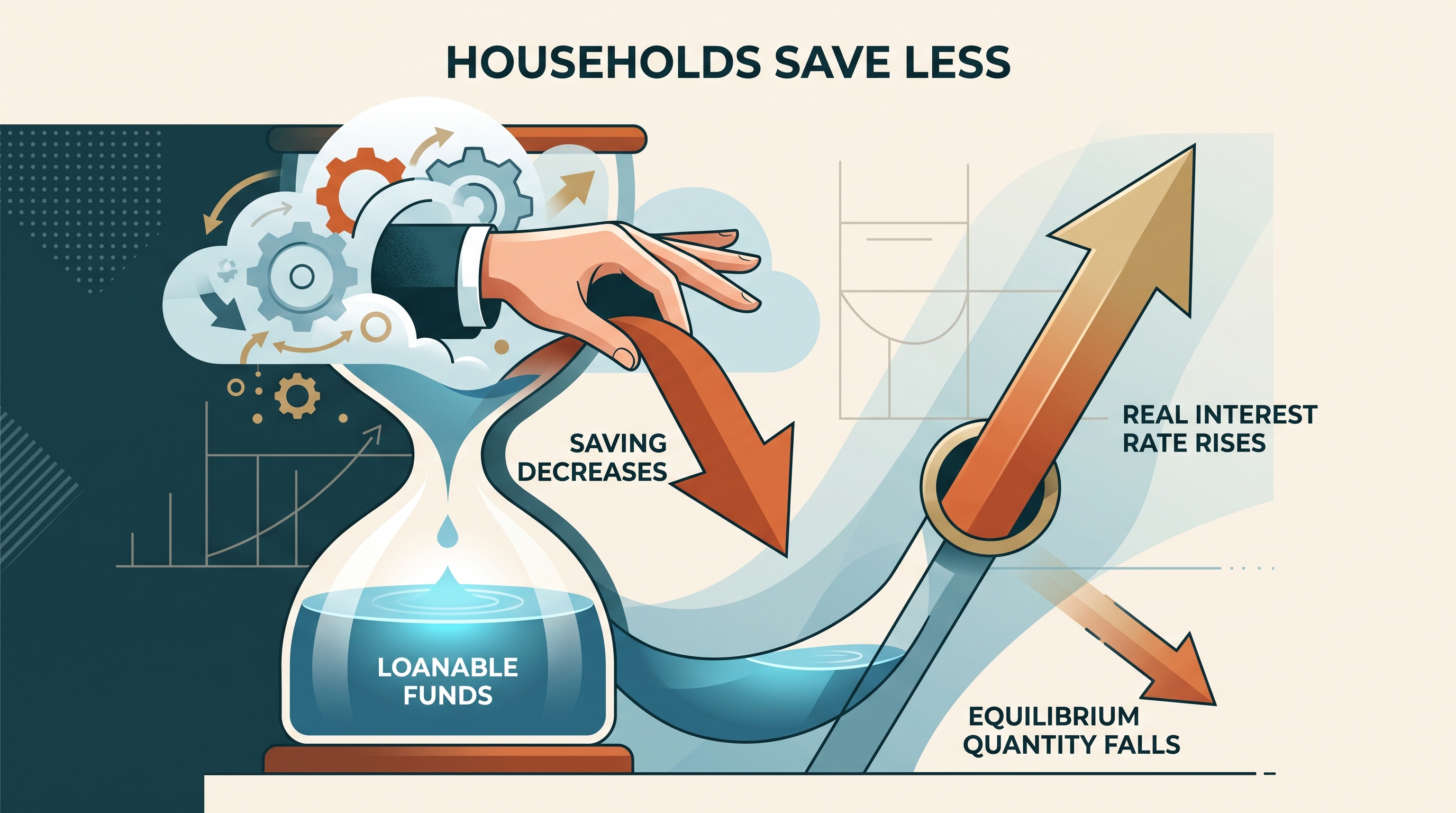
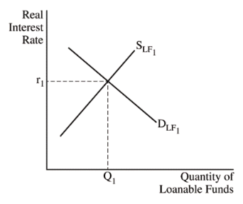
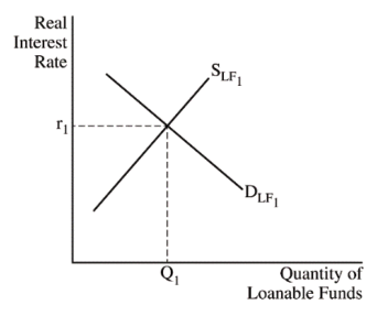
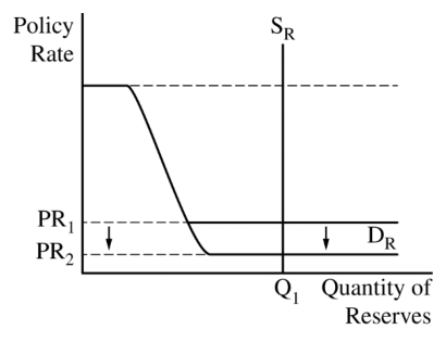
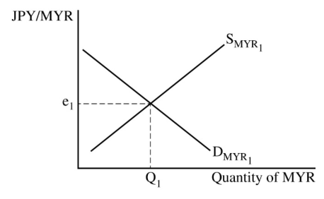
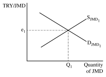
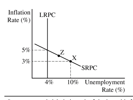
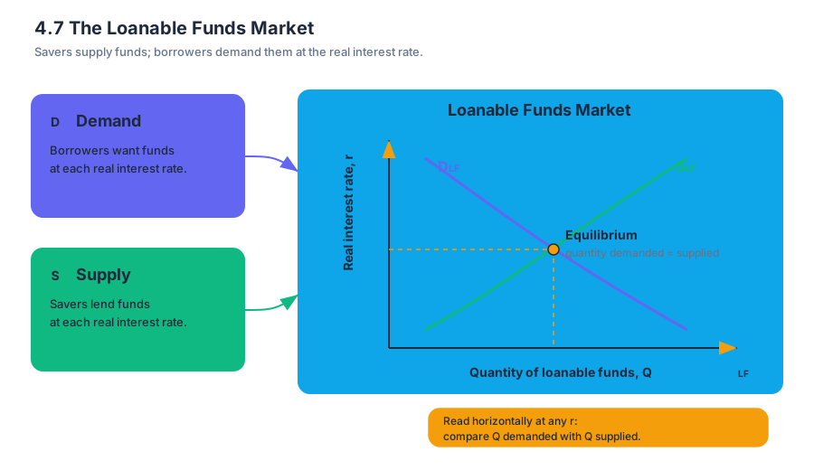
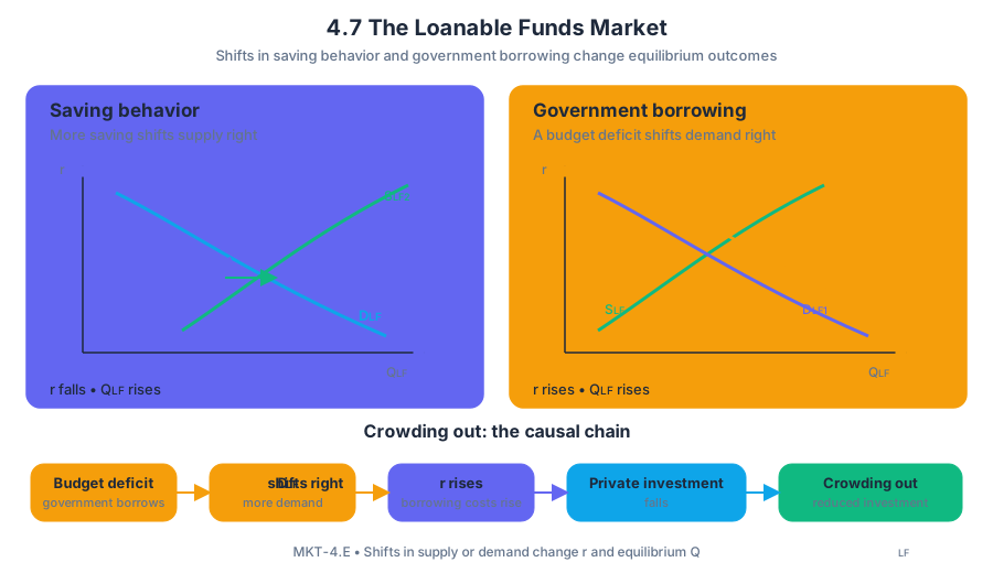
5.1 Fiscal and Monetary Policy Actions in the Short Run
Key concepts: Fiscal policy · Monetary policy · Aggregate demand · Short-run macroeconomic outcomes · Recessionary output gap · Inflationary output gap · Automatic stabilizers · Government deficits · Central banks · Interest on reserves
A recessionary gap means that an economy is producing below its full-employment level, while an inflationary gap means that it is producing above that level.
5.1 Fiscal and Monetary Policy Actions in the Short Run
A recessionary gap means that an economy is producing below its full-employment level, while an inflationary gap means that it is producing above that level. Fiscal and monetary policy can shift aggregate demand, changing short-run real output, the price level, interest rates, and cyclical unemployment.
The policy problem: close the output gap
An output gap is the difference between actual real GDP and potential output, the level of production associated with full employment. If actual output is below potential output, the economy has a negative, or recessionary, output gap. If actual output exceeds potential output, it has a positive, or inflationary, output gap.
Under POL-1.F.1, a combination of expansionary or contractionary policies may restore full employment. Expansionary policy increases aggregate demand and is appropriate for a recessionary gap. Contractionary policy decreases aggregate demand and is appropriate for an inflationary gap.
Under POL-1.F.2, fiscal and monetary policies can influence four connected outcomes: aggregate demand, real output, the price level, and interest rates. The direction of the final result depends on the initial gap and on whether the policies reinforce or offset one another.
Fiscal policy: government spending and taxes
Fiscal policy consists of deliberate changes in government spending, taxes, and transfer payments. Increasing government purchases directly raises aggregate demand because government spending is one component of total spending:
$$Y = C + I + G + NX$$
where $Y$ is real GDP, $C$ is consumption, $I$ is investment, $G$ is government spending, and $NX$ is net exports.
For a recessionary gap, the government can use expansionary fiscal policy by increasing government spending, decreasing taxes, or increasing transfer payments. These actions raise disposable income or directly increase spending, shifting $AD$ rightward. In the short run, real GDP and the price level rise, while cyclical unemployment falls.
For an inflationary gap, the government can use contractionary fiscal policy by decreasing government spending, increasing taxes, or decreasing transfer payments. These actions reduce aggregate demand, lowering the short-run price level and real output toward their sustainable levels.
A fiscal expansion that increases spending or reduces tax revenue can create a government budget deficit. A deficit occurs when government expenditures exceed tax revenues during a period. The deficit is therefore associated with fiscal policy, but it is not itself a policy instrument that automatically determines the economy’s outcome.
Worked example: closing a recessionary gap
Suppose an economy’s potential output is $Y_F = $1{,}000$ billion, but current equilibrium output is $Y_1 = $940$ billion. The recessionary gap is:
$$\text{Output gap} = Y_F - Y_1 = $1{,}000 - $940 = $60\text{ billion}$$
The government increases infrastructure spending. That increase shifts $AD_1$ to the right. The new short-run equilibrium has higher real output and a higher price level. If the spending increase is financed by borrowing, the government budget deficit increases.
At the same time, the central bank lowers interest on reserves. Banks have less incentive to hold reserves, market interest rates tend to fall, and interest-sensitive consumption and investment increase. The resulting increase in spending shifts aggregate demand farther right, reinforcing the fiscal expansion.
Monetary policy and the ample-reserves framework
Monetary policy is the central bank’s use of its tools to pursue macroeconomic goals such as price stability and full employment. Monetary policy affects the money supply and interest rates, which influence consumption and investment and therefore aggregate demand.
In a limited-reserves system, an expansionary open-market purchase increases bank reserves and the money supply, placing downward pressure on interest rates. In an ample-reserves framework, banks already hold substantial reserves, so changing the quantity of reserves may have little effect on the policy rate. Instead, the central bank influences interest rates through administered rates.
The Federal Reserve’s key policy tool in this framework is interest on reserves—the interest rate paid to banks on reserve balances held at the central bank. Decreasing interest on reserves is expansionary: it lowers the opportunity cost of lending, reduces interest rates, increases interest-sensitive spending, and shifts $AD$ rightward. Increasing interest on reserves is contractionary and shifts $AD$ leftward.
A complete monetary-policy explanation must show the entire transmission chain:
$$ \text{Interest on reserves}\downarrow \rightarrow \text{market interest rates}\downarrow \rightarrow I\uparrow \text{ and } C\uparrow \rightarrow AD\uparrow \rightarrow Y\uparrow,\ PL\uparrow,\ \text{cyclical unemployment}\downarrow $$
Automatic stabilizers
Automatic stabilizers are government programs that automatically reduce fluctuations in aggregate demand without requiring a new legislative decision. Progressive income taxes and unemployment benefits are standard examples: during a recession, tax payments fall and benefit payments rise, supporting household disposable income and consumption.
Automatic stabilizers tend to reduce the size of a recessionary gap and restrain an inflationary gap. They do not necessarily eliminate the gap, and they operate through changes in taxes and transfers rather than through a newly enacted discretionary policy.
Policy combinations and common errors
Fiscal and monetary policy can work together. Expansionary fiscal policy raises aggregate demand but may increase interest rates if government borrowing raises demand for loanable funds. Expansionary monetary policy can lower interest rates and partially offset that pressure, supporting investment and consumption.
Misconception check — “Any increase in government spending is always beneficial.” An increase in $G$ is expansionary, but if the economy already has an inflationary gap, it can increase the price level further. Policy must be matched to the initial economic condition.
Misconception check — “Increasing interest on reserves expands the money supply.” In an ample-reserves framework, increasing interest on reserves is contractionary: it raises the policy rate, reduces interest-sensitive spending, and shifts aggregate demand left.
Graphing rule: An AD–AS graph should include a vertical axis labeled Price Level, a horizontal axis labeled Real GDP or Real Output, correctly labeled $AD$ and $SRAS$ curves, the relevant equilibrium points, and arrows showing the direction of the policy-induced shift. A verbal claim without the causal chain or graph may not establish the economic outcome.
Retrieval check
An economy is producing below potential output. Identify one expansionary fiscal action and one expansionary monetary action, then state the short-run effects on $AD$, real output, the price level, and cyclical unemployment. A complete answer should connect each policy to spending before stating the final macroeconomic outcomes. The identifiers for this reasoning are POL-1.F.1, POL-1.F.2, and POL-12.B.
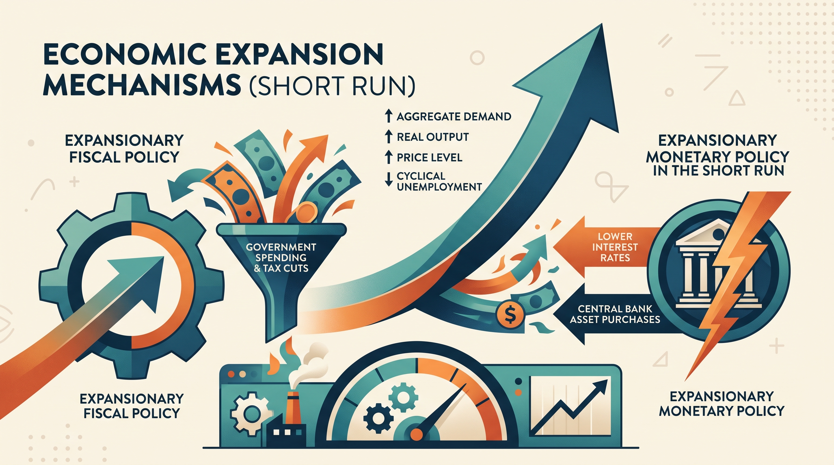
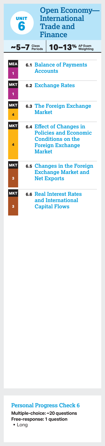
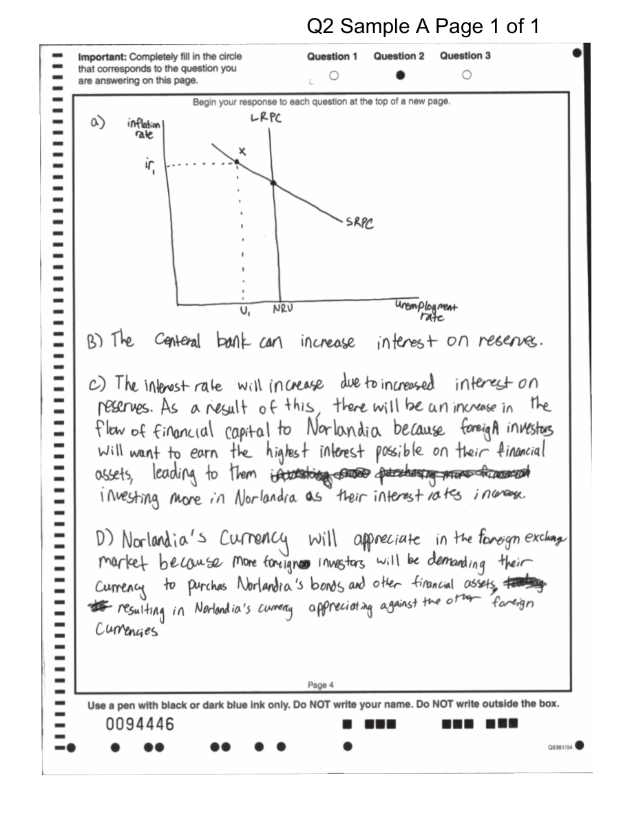
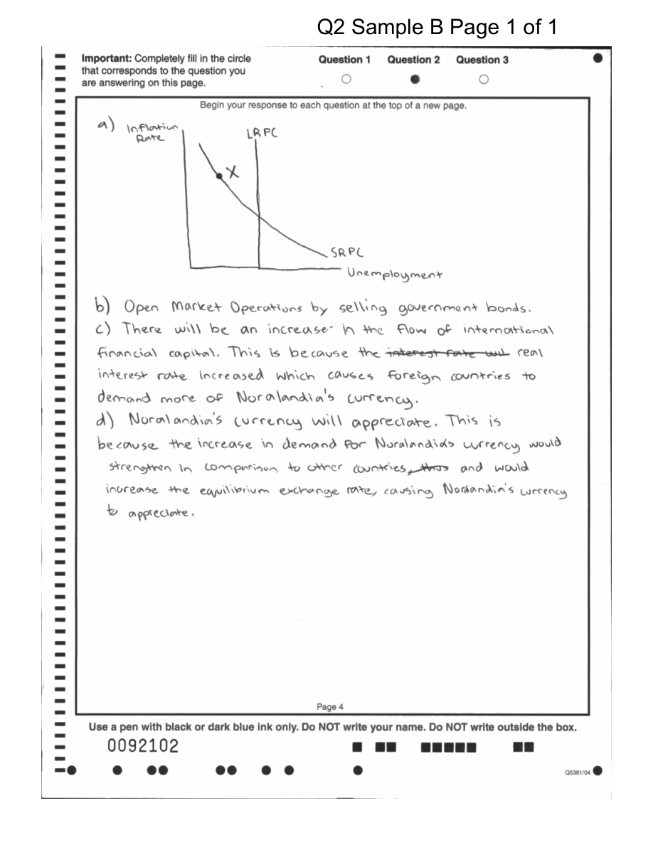
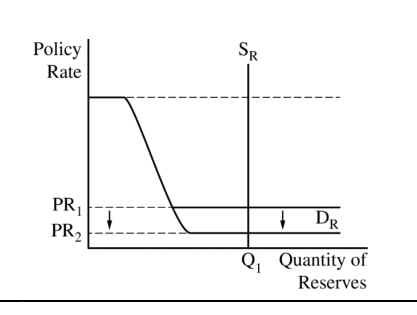
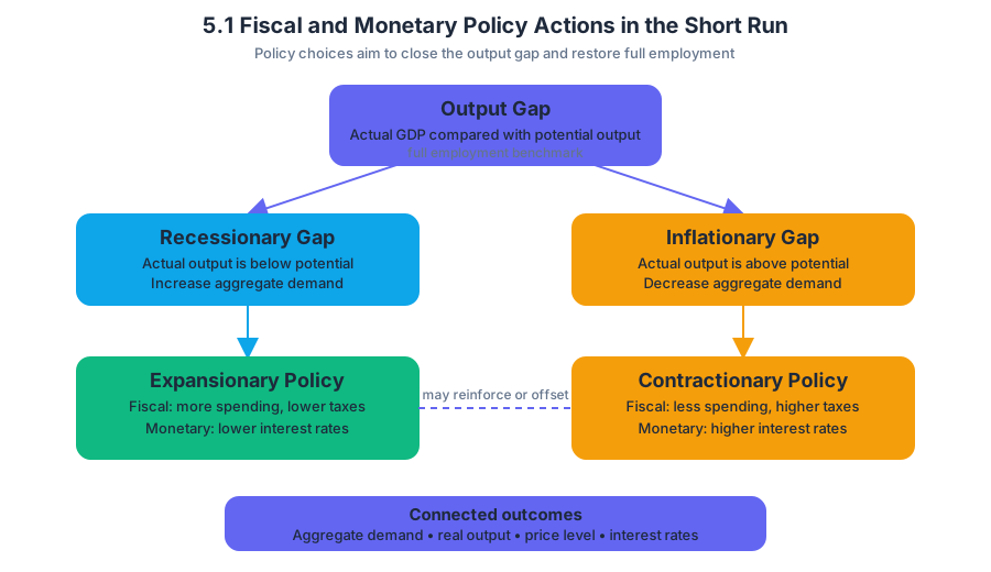
5.2 The Phillips Curve
Key concepts: Short-run Phillips curve (SRPC) · Long-run Phillips curve (LRPC) · Natural rate of unemployment · Actual unemployment rate · Cyclical unemployment · Structural unemployment · Natural unemployment · Graphing Phillips curve relationships · Distinguishing short-run and long-run outcomes · Common errors in calculating unemployment rates
The Phillips curve models the relationship between inflation and unemployment: in the short run, higher inflation is associated with lower unemployment, but in the long run unemployment returns to a rate determined by the economy’s labor-market structure.
5.2 The Phillips Curve
The Phillips curve models the relationship between inflation and unemployment: in the short run, higher inflation is associated with lower unemployment, but in the long run unemployment returns to a rate determined by the economy’s labor-market structure.
The two curves
The short-run Phillips curve (SRPC) is downward sloping. Its horizontal axis measures the unemployment rate, and its vertical axis measures the inflation rate. Moving along the SRPC represents a short-run trade-off: stronger demand can raise production and employment while also increasing the price level and inflation.
The long-run Phillips curve (LRPC) is vertical at the natural rate of unemployment. In the long run, there is no permanent trade-off between inflation and unemployment. Changes in aggregate demand may move the economy to a different point on a short-run curve, but unemployment ultimately returns to the natural rate.
The intersection of the SRPC and LRPC represents long-run equilibrium. Points to the left of the LRPC have unemployment below the natural rate and represent an inflationary gap. Points to the right have unemployment above the natural rate and represent a recessionary gap; this distinction is formalized in MOD-3.A.5.
Natural versus actual unemployment
Natural unemployment is the unemployment that remains even when the economy is producing at full employment. It consists of frictional unemployment, caused by normal job search and transitions, plus structural unemployment, caused by a mismatch between workers’ skills or locations and available jobs:
$$ \text{Natural unemployment}=\text{frictional unemployment}+\text{structural unemployment} $$
The natural rate of unemployment is the natural amount expressed as a percentage of the labor force. The actual unemployment rate is the unemployment rate currently observed in the economy. Their difference is cyclical unemployment, which rises during recessions and falls during expansions:
$$ \text{Cyclical unemployment}=\text{Actual unemployment rate}-\text{Natural rate of unemployment} $$
Therefore, the correct relationship is:
$$ \text{Actual unemployment rate}=\text{Natural rate of unemployment}+\text{Cyclical unemployment} $$
Structural unemployment is already included in the natural rate. It must not be added again.
Misconception check: The actual unemployment rate is not calculated by adding cyclical, natural, and structural unemployment. It is also not calculated by adding only cyclical and structural unemployment. Adding structural unemployment separately double-counts it because structural unemployment is already part of the natural rate.
Reading points on the graph
Suppose an economy’s natural rate of unemployment is $6%$. A temporary boom reduces the actual unemployment rate to $4%$, while inflation rises to $7%$. On the Phillips curve graph, locate the point at $4%$ unemployment and $7%$ inflation. Because $4%$ is below the natural rate, the point lies to the left of the vertical LRPC and represents an inflationary gap.
The cyclical unemployment rate is:
$$ 4%-6%=-2% $$
A negative cyclical unemployment rate does not mean that total unemployment is negative. It means actual unemployment is $2$ percentage points below the natural rate.
Now consider a supply shock, such as a sudden increase in energy costs. A supply shock raises firms’ production costs and can create higher inflation and higher unemployment simultaneously. In the Phillips curve model, this is represented by a shift of the SRPC, not movement along the existing SRPC. By contrast, a demand shock corresponds to movement along the SRPC (MOD-3.B.1 and MOD-3.B.2).
Why the LRPC can move
The LRPC shifts when the natural rate of unemployment changes. For example, widespread improvements in job-matching technology could reduce frictional unemployment, shifting the LRPC leftward. A lasting increase in skill mismatch could raise structural unemployment, shifting the LRPC rightward (MOD-3.B.3).
This is why the natural rate is not a fixed unemployment number. It depends on labor-market institutions, worker skills, geographic mobility, information about jobs, and the time required to match workers with employers.
Graphing protocol
For an AP graph, label the vertical axis Inflation rate (%) and the horizontal axis Unemployment rate (%). Draw a downward-sloping SRPC, a vertical LRPC at the natural rate, and label the relevant point on the SRPC. Then state whether the point lies left or right of the LRPC and connect that position to an inflationary or recessionary gap.
A complete explanation might read: “The point lies to the right of the LRPC, so the actual unemployment rate exceeds the natural rate. Cyclical unemployment is positive, indicating a recessionary gap.” This graph-and-causal-chain work is connected to the topic’s official learning objectives OD-3, MKT-4, POL-3, GMEA-2, AMOD-3, and BPOL-3.
Retrieval check
An economy has a natural rate of unemployment of $5%$ and an actual unemployment rate of $3%$. Is cyclical unemployment positive or negative? Where is the point located relative to the LRPC, and what type of gap does it represent?
Answer: Cyclical unemployment is $3%-5%=-2%$. The point lies to the left of the LRPC and represents an inflationary gap.
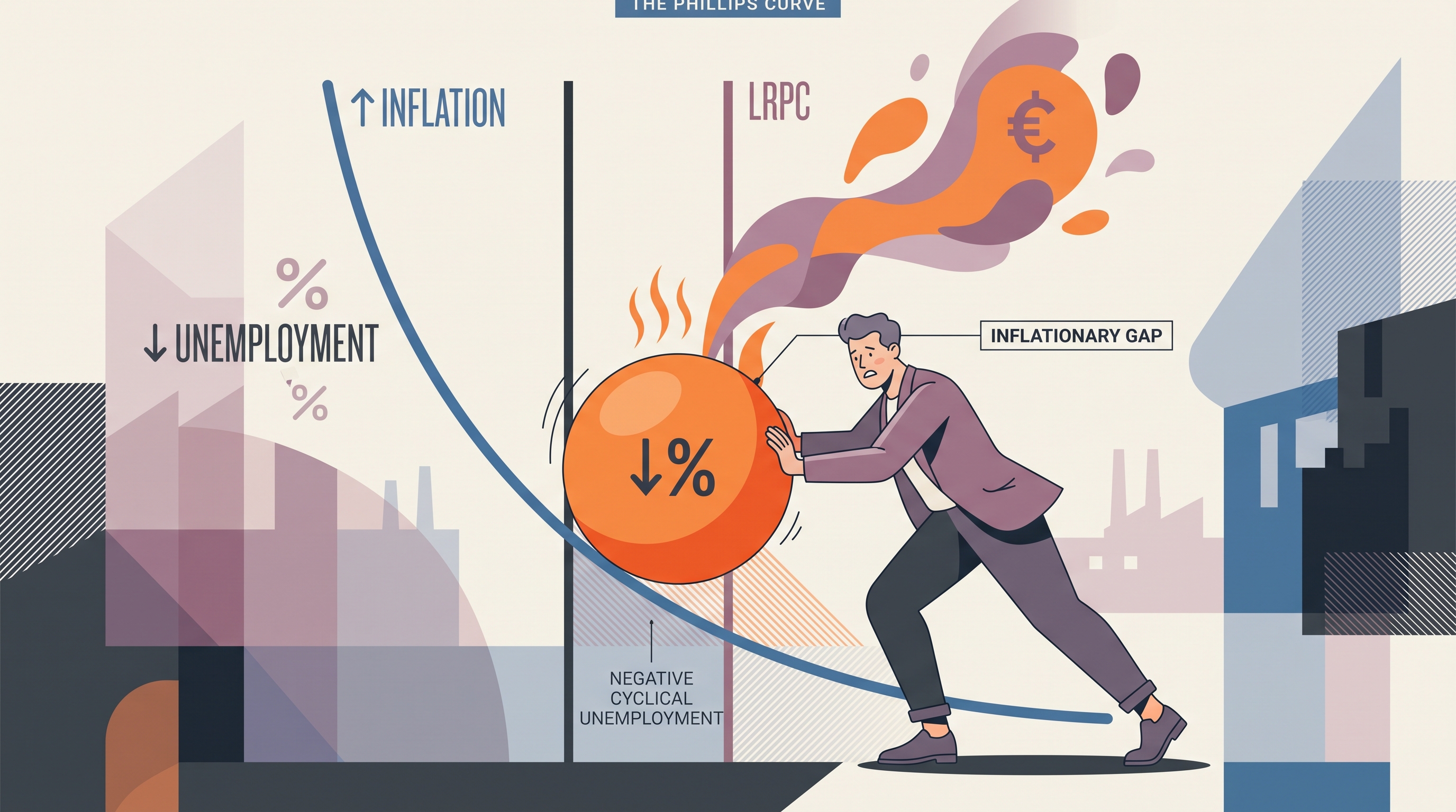
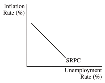
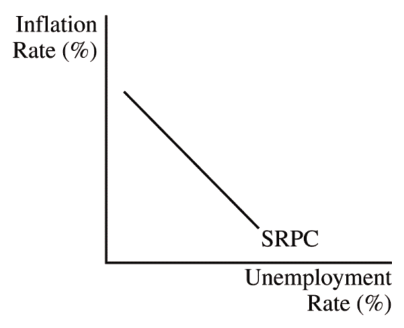
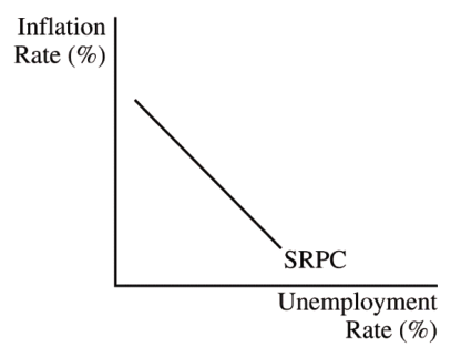
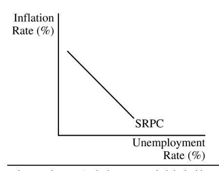
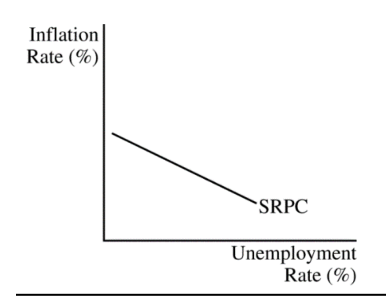
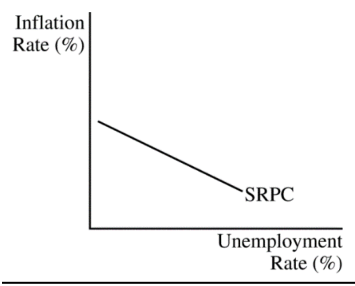
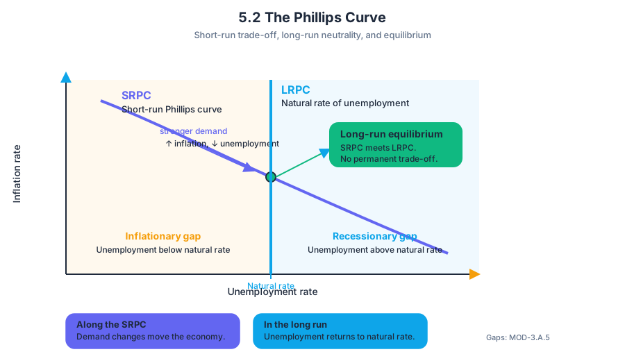
5.3 Money Growth and Inflation
When the quantity of money grows faster than the economy’s production of goods and services, the average price level tends to rise. The central question is therefore: How can more money chasing roughly the same output reduce the purchasing power of each monetary unit?
5.3 Money Growth and Inflation
When the quantity of money grows faster than the economy’s production of goods and services, the average price level tends to rise. The central question is therefore: How can more money chasing roughly the same output reduce the purchasing power of each monetary unit?
The quantity theory of money
Imagine a small island economy producing exactly $100$ smoothies in a year. If the money used to purchase those smoothies rises from $1{,}000$ to $2{,}000$ while smoothie production stays at $100$, sellers can charge more per smoothie without producing anything additional. The economy has more spending power, but not more products.
Quantity theory of money: In the long run, a sustained increase in the money supply, with other important factors held constant, tends to produce a proportional increase in the price level.
The relationship is represented by the equation
$$MV = PY$$
where:
- $M$ is the money supply, the quantity of money available for transactions;
- $V$ is the velocity of money, the average number of times each unit of money is used to purchase final goods and services;
- $P$ is the price level;
- $Y$ is real output, or the quantity of goods and services produced.
From money growth to inflation
Because nominal GDP equals the price level multiplied by real output, $PY$ is also nominal GDP. If velocity is stable, the equation implies that money growth must be connected to nominal GDP growth:
$$\text{growth in }M+\text{growth in }V\approx\text{inflation rate}+\text{growth in }Y$$
If velocity does not change, this simplifies to
$$\text{inflation rate}\approx\text{money-supply growth rate}-\text{real-output growth rate}$$
Worked example. Suppose the money supply increases by $8%$, velocity remains unchanged, and real output increases by $3%$. The approximate inflation rate is
$$8%-3%=5%$$
The economy can absorb about $3%$ more money through increased production. The remaining $5%$ is associated with a higher price level. If real output instead grew by $8%$, the approximate inflation rate would be $0%$, assuming velocity stayed constant.
Why the result is mainly long-run
In the short run, an increase in the money supply can lower interest rates and encourage borrowing, consumption, and investment. Those changes can increase aggregate demand and raise real output as firms respond to stronger sales. This is why money growth does not instantly translate one-for-one into inflation.
Over time, however, wages and input prices adjust, productive capacity becomes the limiting factor, and real output is determined mainly by resources, technology, and institutions rather than by the number of dollars in circulation. Once the economy returns toward its long-run output level, continued money growth primarily raises the price level.
Money neutrality
Money neutrality is the long-run idea that changes in the money supply affect nominal variables—such as the price level, nominal wages, and nominal GDP—but do not permanently change real variables—such as real GDP, employment at the natural rate, or the economy’s productive capacity.
For example, if the money supply doubles while real output and velocity remain unchanged, the quantity equation requires the price level to double:
$$M_2=2M_1 \quad\Rightarrow\quad P_2=2P_1$$
The numerical prices and wages may be larger, but the economy has not automatically gained more factories, workers’ skills, land, or technology.
Misconception check: “More money always creates more real wealth”
Named misconception — money illusion: A larger dollar amount is not necessarily greater purchasing power. If a worker’s nominal wage rises by $6%$ while the price level rises by $6%$, the worker’s real wage is approximately unchanged. The worker has more dollars but can buy roughly the same quantity of goods and services.
A second misconception is that the quantity equation proves inflation must equal money-supply growth in every period. It does not. The relationship depends on velocity and real output. A change in payment habits can alter $V$, while productivity changes can alter $Y$; both affect the inflation outcome.
AP skill focus: POL (3) — Manipulation
Topic 5.3 Money Growth and Inflation is categorized as POL (3): POL identifies the big idea Macroeconomic Policies, and 3 identifies Skill Category 3, Manipulation. This skill requires using economic relationships, equations, and numerical information to determine how a change in one variable affects another.
On an exam, manipulate the quantity equation in a disciplined order:
- Identify whether the prompt gives changes in $M$, $V$, $P$, or $Y$.
- Write the growth-rate relationship.
- Hold velocity constant only when the question states or implies that assumption.
- Substitute the numbers and identify whether the result is inflation or deflation.
- Distinguish a change in nominal values from a change in real output.
Retrieval check
An economy’s money supply grows by $10%$, velocity falls by $2%$, and real output grows by $4%$. Using the growth-rate form of $MV=PY$, estimate the inflation rate.
The answer is
$$10%-2%-4%=4%$$
Money growth raises nominal spending, the velocity decline reduces it, and real-output growth absorbs part of the remaining spending increase. Thus the approximate price-level growth is $4%$, not $10%$.
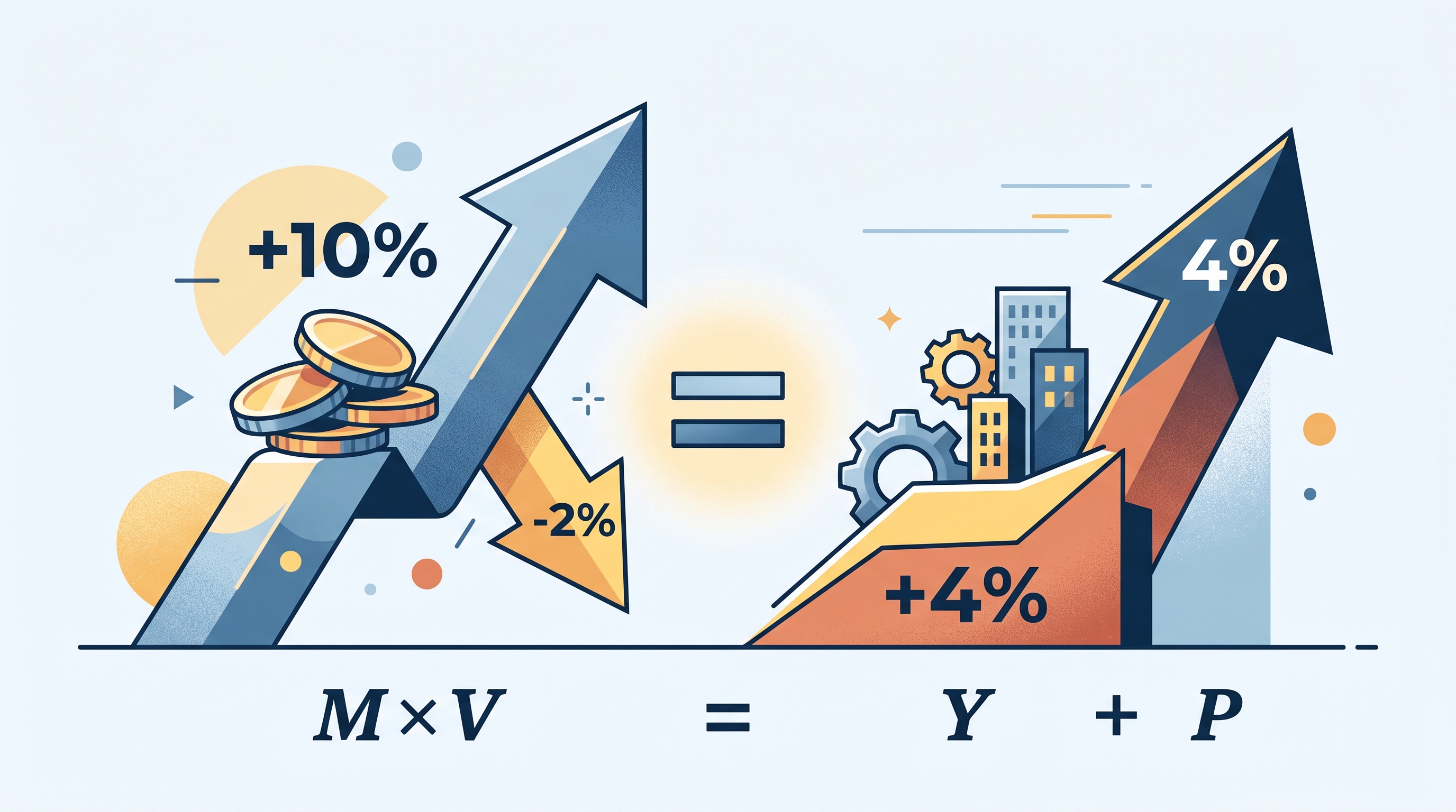
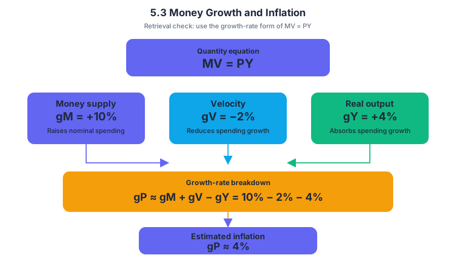
5.4 Government Deficits and the National Debt
Key concepts: Government budget surplus or deficit · Budget deficit and national debt · Government interest payments on accumulated debt · Opportunity cost of debt interest payments · Crowding out · Long-run implications of fiscal policy
A government runs a budget deficit when, during a given year, its purchases and transfer payments exceed the tax revenue it collects. The deficit is a one-year flow; the national debt is the accumulated total of past borrowing, a stock that persists over time.
5.4 Government Deficits and the National Debt
A government runs a budget deficit when, during a given year, its purchases and transfer payments exceed the tax revenue it collects. The deficit is a one-year flow; the national debt is the accumulated total of past borrowing, a stock that persists over time.
The annual government budget
The government budget surplus or deficit is calculated as:
$$ \text{Budget surplus or deficit}=T-(G+TR) $$
where $T$ represents tax revenues, $G$ represents government purchases, and $TR$ represents transfer payments. A positive result is a surplus; a negative result is a deficit.
Learning Objective POL-3.B: Define the government budget surplus (deficit) and national debt, and explain the issues involved in the burden of the national debt.
Essential Knowledge POL-3.B.1: The government budget surplus (deficit) is the difference between tax revenues and government purchases plus transfer payments in a given year.
A useful visual distinction is:
| Annual budget position | Calculation | Immediate meaning |
|---|---|---|
| Budget surplus | $T-(G+TR)>0$ | Tax revenue exceeds purchases plus transfers |
| Balanced budget | $T-(G+TR)=0$ | Revenue equals purchases plus transfers |
| Budget deficit | $T-(G+TR)<0$ | Purchases plus transfers exceed tax revenue |
Worked example: Fehran
Suppose Fehran collects $110$ billion in taxes and makes $90$ billion in government purchases while paying $50$ billion in transfer payments. Its budget result is:
$$ T-(G+TR)=110-(90+50)=110-140=-30 $$
Fehran has a budget deficit of $30$ billion because government outlays are greater than taxes. It must finance that gap by borrowing, assuming it does not use previously accumulated financial assets.
Manipulation — Skill 3: Manipulation is central here: change one component of the expression and determine the outcome. If Fehran raises taxes by $20$ billion, the deficit falls from $30$ billion to $10$ billion. If instead it increases purchases by $20$ billion, the deficit grows to $50$ billion.
From a deficit to national debt
Essential Knowledge POL-3.B.2: A government adds to the national debt when it runs a budget deficit.
The deficit is the addition made during one year; the national debt is the total accumulated balance. All else equal, a surplus reduces the national debt, while a deficit increases it.
$$ \text{Debt}_{t}
\text{Debt}_{t-1} + \text{Current deficit}
\text{Current surplus} $$
For Fehran, if the national debt began at $800$ billion, the $30$ billion deficit raises it to $830$ billion. A later $12$ billion surplus would reduce the debt to $818$ billion, not erase the entire debt.
Misconception check — “The deficit and the debt are the same thing.”
They are not. A deficit is a yearly shortfall; the debt is the accumulated result of many shortfalls, less any surpluses.
Interest payments and opportunity cost
Essential Knowledge POL-3.B.3: A government must pay interest on its accumulated debt, thus increasing the national debt and increasingly forgoing those funds for alternative uses.
Borrowing creates a continuing obligation. If Fehran owes $830$ billion and must make $40$ billion in interest payments, those payments require government funds; if they are financed through additional borrowing, the debt rises further.
The economic burden is not simply the existence of a large number. Interest payments have an opportunity cost: money used to service existing debt cannot simultaneously fund infrastructure, education, emergency relief, tax reductions, or other public priorities. As debt accumulates, interest obligations can claim a larger share of the budget.
Long-run implications and the bridge to crowding out
Enduring Understanding POL-3: There are long-run implications of monetary and fiscal policy. Persistent deficits can increase borrowing, raise future interest obligations, and limit later policy choices.
When government borrowing competes with private borrowers for available loanable funds, it can reduce private investment or other interest-sensitive spending. This adverse effect is called crowding out; the detailed loanable-funds mechanism belongs to POL-3.C, but the causal starting point is established here: deficit spending usually requires borrowing.
Retrieval check: If $T=500$, $G=360$, and $TR=190$, is the government running a surplus or deficit, and by how much?
Answer: $500-(360+190)=-50$, so it is running a $50$ billion deficit. The national debt increases by $50$ billion, all else equal, before considering any further effects such as interest payments.
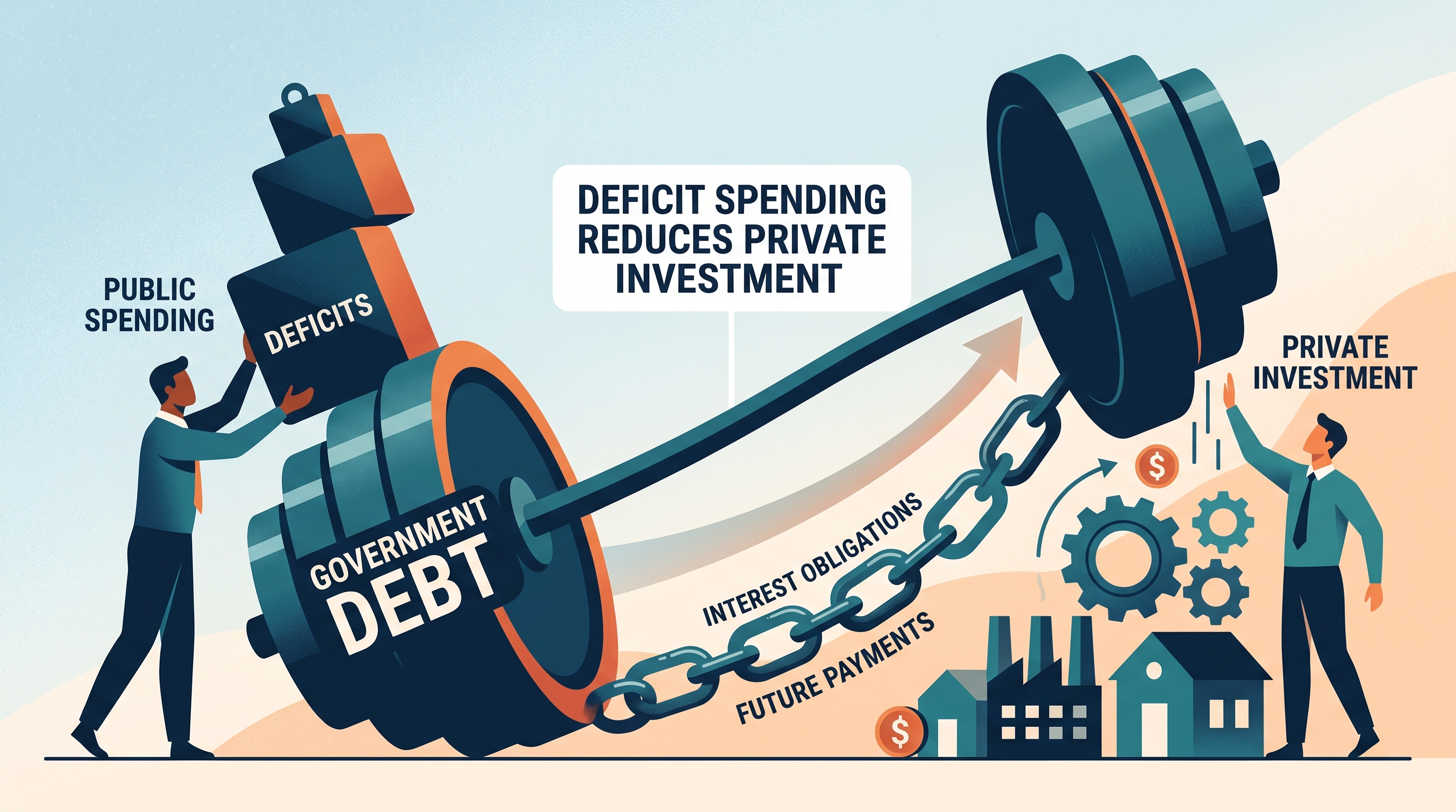
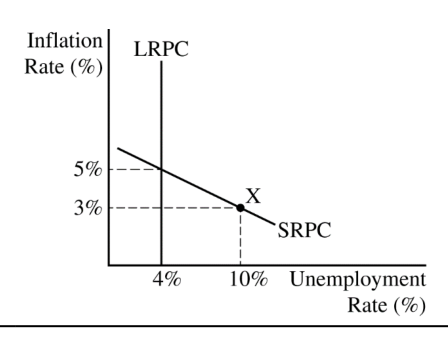
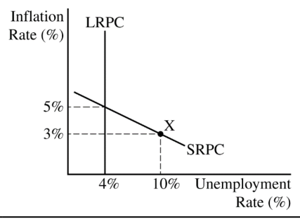
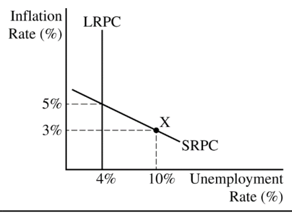
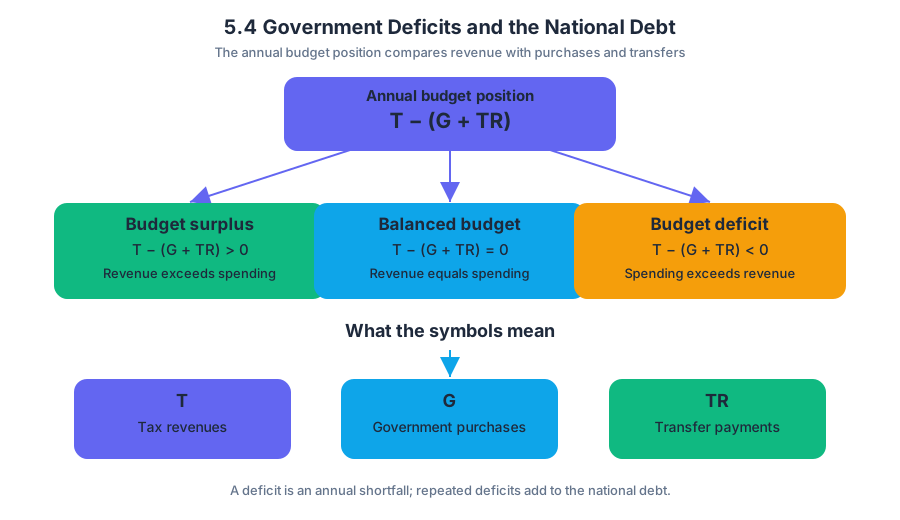
5.5 Crowding Out
When the government finances a budget deficit by selling bonds, its additional borrowing increases demand for loanable funds. If the supply of saving does not increase enough to match that demand, the real interest rate rises and some private investment is displaced—a process called crowding out.
5.5 Crowding Out
When the government finances a budget deficit by selling bonds, its additional borrowing increases demand for loanable funds. If the supply of saving does not increase enough to match that demand, the real interest rate rises and some private investment is displaced—a process called crowding out.
Crowding out is the reduction in private investment caused by higher real interest rates when government borrowing increases demand in the loanable-funds market.
The loanable-funds mechanism
The loanable-funds market connects savers who supply funds with borrowers who demand funds. The market’s price is the real interest rate, because borrowers and lenders care about the purchasing power of repayment rather than merely the number of dollars repaid.
In the standard graph, the vertical axis measures the real interest rate, $r$, and the horizontal axis measures the quantity of loanable funds, $Q_{LF}$. The supply curve represents saving; the demand curve represents borrowing for private investment and government deficits.
When the government finances that gap by selling bonds, its additional borrowing shifts the demand for loanable funds to the right. The equilibrium real interest rate rises from $r_1$ to $r_2$. At the higher interest rate, private firms borrow less for factories, equipment, research, or new buildings, so private investment falls from $I_1$ to $I_2$.
$$ \text{Government borrowing} \uparrow ;\Rightarrow; D_{LF} \text{ shifts right} ;\Rightarrow; r \uparrow ;\Rightarrow; \text{private investment} \downarrow $$
Worked example: tracing the displacement
Suppose the initial loanable-funds equilibrium has a real interest rate of $3%$. Firms plan to borrow $500$ billion for private investment, while households and other institutions supply that amount through saving. The government then borrows an additional $100$ billion by selling bonds.
The government’s borrowing shifts the demand curve rightward. Assume the new equilibrium real interest rate is $5%$. At $5%$, firms now find only $450$ billion of investment projects profitable enough to undertake.
The outcome is:
$$ \Delta I = I_2-I_1 $$
$$ \Delta I = $450\text{ billion}-$500\text{ billion} = -$50\text{ billion} $$
Private investment has fallen by $50$ billion. That $50$ billion is the amount of crowding out in this example—not the entire $100$ billion borrowed by the government. Government borrowing increased total demand for loanable funds, but the higher real interest rate prevented some private borrowers from obtaining funds on acceptable terms.
Why crowding out matters for aggregate demand
In the short run, expansionary fiscal policy can increase aggregate demand because higher government spending raises one component of planned expenditure. However, if the resulting government borrowing raises real interest rates, lower private investment offsets part of that increase.
$$ AD = C + I + G + NX $$
If $G$ rises while $I$ falls, aggregate demand still may increase, but by less than it would have increased without crowding out. This is why crowding out reduces the size of fiscal policy’s effect rather than automatically reversing it.
Crowding out can be stronger when the supply of loanable funds is relatively unresponsive to the interest rate. It can be weaker when households save more, foreign lenders supply funds, or the economy has substantial unused saving capacity.
Common misconception: “All government borrowing crowds out investment completely”
Correction: Crowding out is usually partial in the basic model. Government borrowing raises the real interest rate and reduces private investment, but it does not necessarily reduce private investment dollar-for-dollar. The final effect depends on the slopes and positions of the loanable-funds curves.
A second misconception is that a higher nominal interest rate proves crowding out. The loanable-funds model focuses on the real interest rate:
$$ r \approx i-\pi^e $$
where $i$ is the nominal interest rate and $\pi^e$ is expected inflation. A change in the nominal rate does not by itself establish that borrowing has become more expensive in real terms.
AP reasoning and graphing
This topic directly exercises Skill Category 3: Manipulation, especially 3.A, applying economic models to determine how a change shifts a curve or changes an equilibrium. On a loanable-funds graph, a strong response identifies the rightward shift of demand, the higher equilibrium real interest rate, and the lower quantity of private investment.
It also uses 3.B, explaining an economic chain in words and symbols: government borrowing increases demand for loanable funds; the real interest rate rises; private investment decreases. A complete graph must label the axes, identify the original and new equilibrium, show the demand shift, and mark the change in the real interest rate.
Retrieval check
A government begins borrowing more while the supply of loanable funds remains unchanged. Predict the effects on the loanable-funds graph and private investment.
Answer: Demand for loanable funds shifts right, the equilibrium real interest rate rises, and private investment falls. The fall in private investment is crowding out.
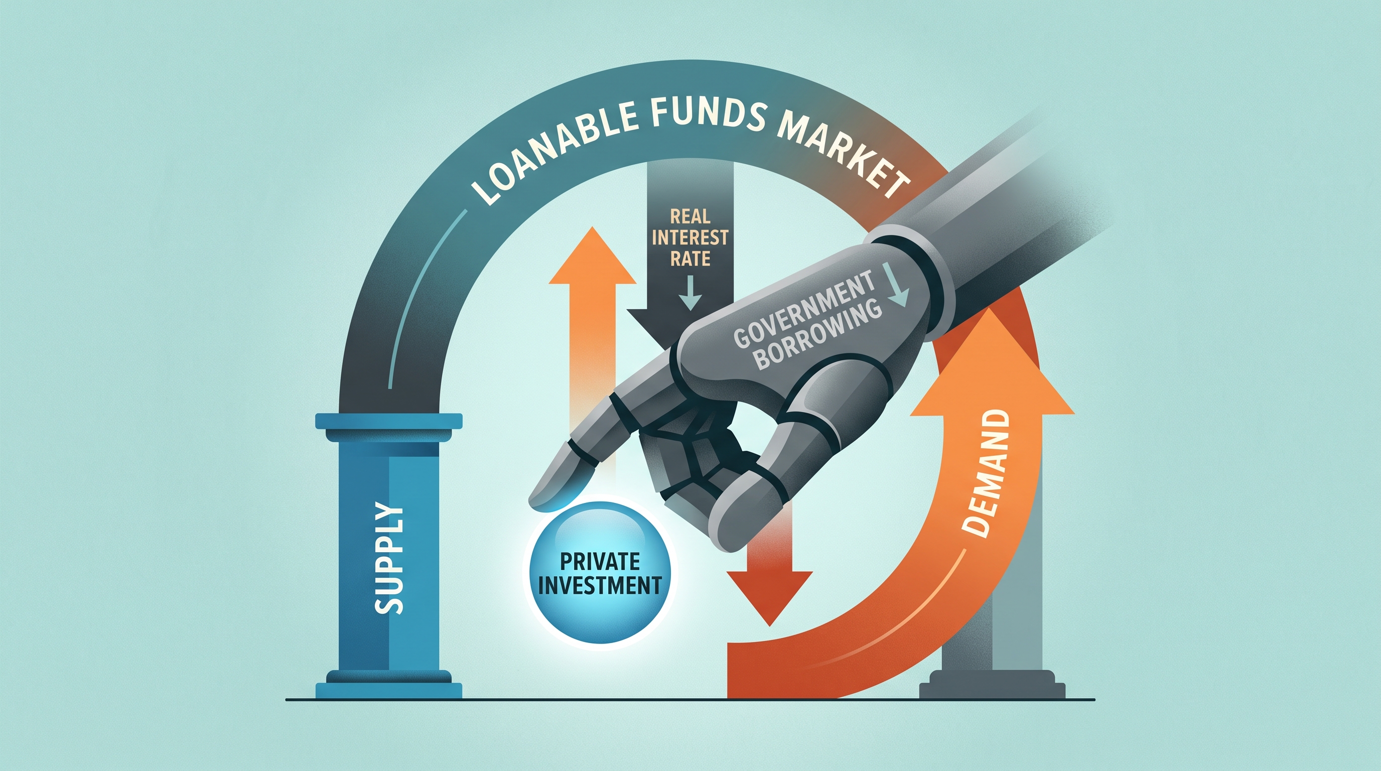
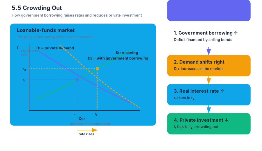
5.6 Economic Growth
Economic growth is an increase in an economy’s ability to produce goods and services over time. The key question is not merely whether a country produces more dollars of output, but whether it can produce more real output per person without mistaking higher prices for greater production.
5.6 Economic Growth
Economic growth is an increase in an economy’s ability to produce goods and services over time. The key question is not merely whether a country produces more dollars of output, but whether it can produce more real output per person without mistaking higher prices for greater production.
CED alignment: Topic 5.6 Economic Growth; Learning Objective 5.6.A Explain how economic growth is measured; Learning Objective 5.6.B Explain the determinants of economic growth; Big Idea MEA: Economic Measurements; Skill Category 1: Principles and Models, 2: Interpretation, 3: Manipulation, and 4: Graphing and Visuals.
Measuring growth: real output, not inflated prices
The standard measure of economic growth is the percentage change in real GDP, which values current production using constant prices. Real GDP is essential because nominal GDP can rise even when an economy produces the same quantity of goods and services at higher prices.
$$ \text{Economic growth rate}
\frac{\text{Real GDP}{\text{new}}-\text{Real GDP}{\text{old}}} {\text{Real GDP}_{\text{old}}} \times 100 $$
For living standards, economists usually examine real GDP per capita—real GDP divided by the population. Total real GDP may increase while real GDP per capita falls if population growth is faster than output growth.
$$ \text{Real GDP per capita}
\frac{\text{Real GDP}}{\text{Population}} $$
Worked example. Suppose an economy’s real GDP rises from $$800$ billion to $$840$ billion while its population rises from $100$ million to $105$ million.
$$ \text{Real GDP growth}
\frac{840-800}{800}\times 100
5% $$
$$ \text{Old real GDP per capita}
\frac{$800\text{ billion}}{100\text{ million}}
$8{,}000 $$
$$ \text{New real GDP per capita}
\frac{$840\text{ billion}}{105\text{ million}}
$8{,}000 $$
Total real GDP grew by $5%$, but real GDP per capita did not change. The economy became larger, not more productive per person. This distinction is why economic growth and improvements in average material living standards are related but not identical.
What produces economic growth?
Under CED Essential Knowledge 5.6.B.1, long-run economic growth results when an economy’s productive capacity expands. In the production possibilities model, growth appears as an outward shift of the production possibilities curve (PPC). In the AD–AS model, sustained growth is represented by a rightward shift of long-run aggregate supply (LRAS).
The principal determinants of growth are:
- Physical capital: tools, factories, machines, infrastructure, and equipment used to produce output.
- Human capital: workers’ education, training, skills, and health.
- Natural resources: land, minerals, energy, and other inputs supplied by nature.
- Technology: knowledge and methods that allow existing resources to produce more output or produce it at lower cost.
Investment in physical and human capital can raise productivity, meaning output produced per worker or per hour. Technological progress is especially powerful because it can improve the efficiency of many workers and machines simultaneously.
Worked contextual example. A country builds a modern port, trains logistics workers, and adopts software that coordinates shipments. The port is physical capital; worker training creates human capital; the software is a technological improvement. Together, these changes allow the economy to produce and transport more output at every possible price level, shifting LRAS rightward and expanding the PPC.
Graphing the growth mechanism
On a PPC graph, economic growth is shown by the entire curve shifting outward. A movement from an interior point to the existing curve represents better use of idle resources, not economic growth. Growth requires an increase in the economy’s maximum sustainable output.
On an AD–AS graph, long-run growth shifts LRAS from $LRAS_1$ to $LRAS_2$. If aggregate demand remains unchanged, the price level may fall while real output rises. If aggregate demand also increases, both real output and the price level may rise; the output increase still reflects greater productive capacity.
Misconception check
Misconception: “A higher nominal GDP always means economic growth.” Not necessarily. If prices rise by $8%$ while nominal GDP rises by $8%$, real GDP may be unchanged. Always separate changes in quantities from changes in prices.
Misconception: “Economic growth automatically benefits every person equally.” Real GDP per capita is an average. It does not reveal income distribution, unpaid household production, environmental costs, or whether gains are concentrated among a small group. Those limitations do not make the measure useless; they explain why it must be interpreted carefully.
Skills in action
Topic 5.6 is assessed through 1.A Define economic principles and models, 1.B Explain economic principles, concepts, and models, and 1.C Apply economic concepts, principles, and models when identifying growth and connecting capital or technology to productive capacity. 2.C Use quantitative data to evaluate economic outcomes and 3.C Calculate and interpret economic measures are used when computing real GDP growth or real GDP per capita. 4.A Draw correctly labeled graphs and 4.C Analyze graphical representations are used to show and interpret outward shifts of the PPC or LRAS.
Retrieval check
An economy’s real GDP rises by $4%$, but its population rises by $6%$. Did real GDP per capita increase? No. Because population grew faster than real GDP, real GDP per capita decreased. A complete answer should distinguish total economic growth from growth in output per person.
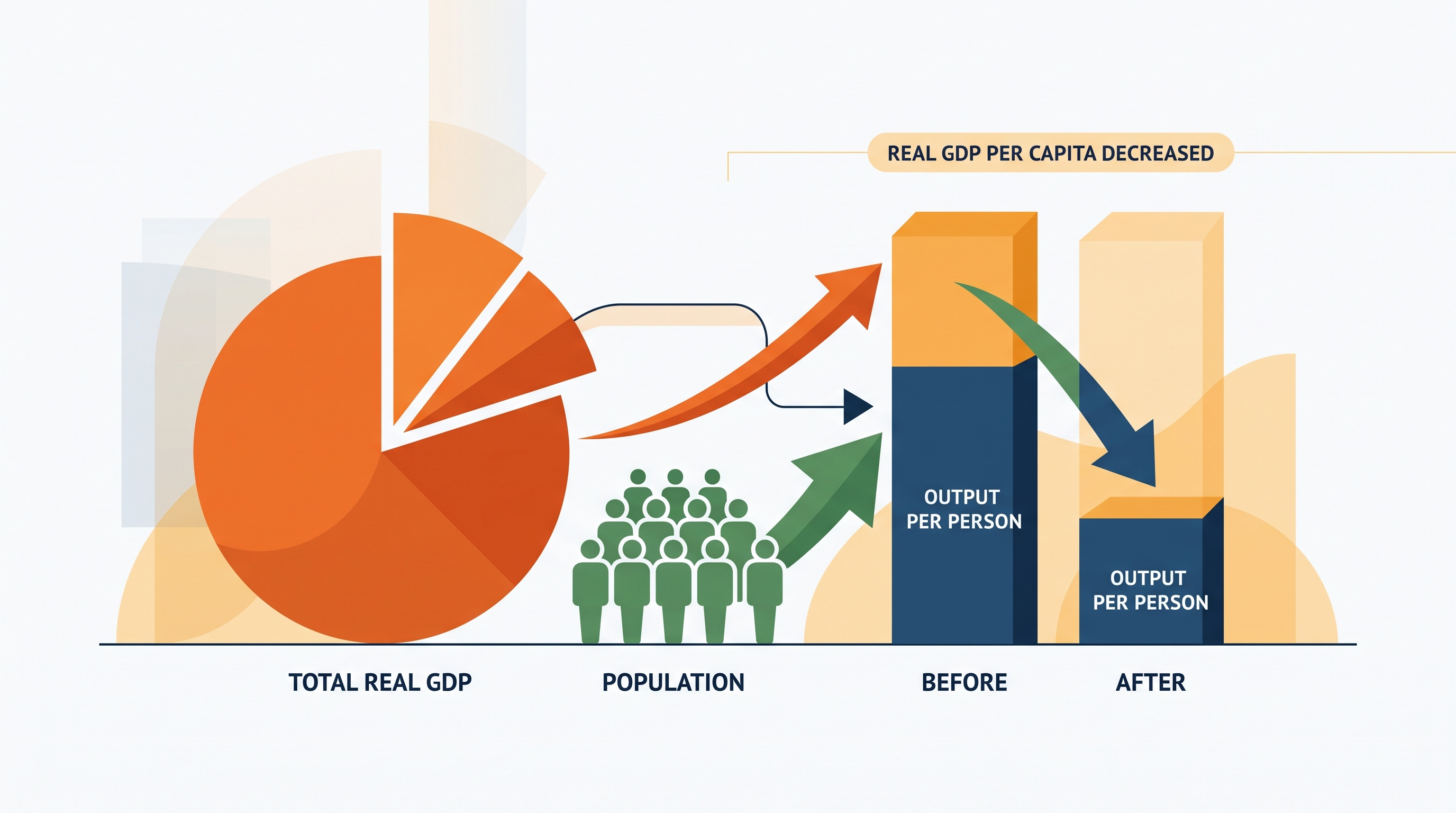
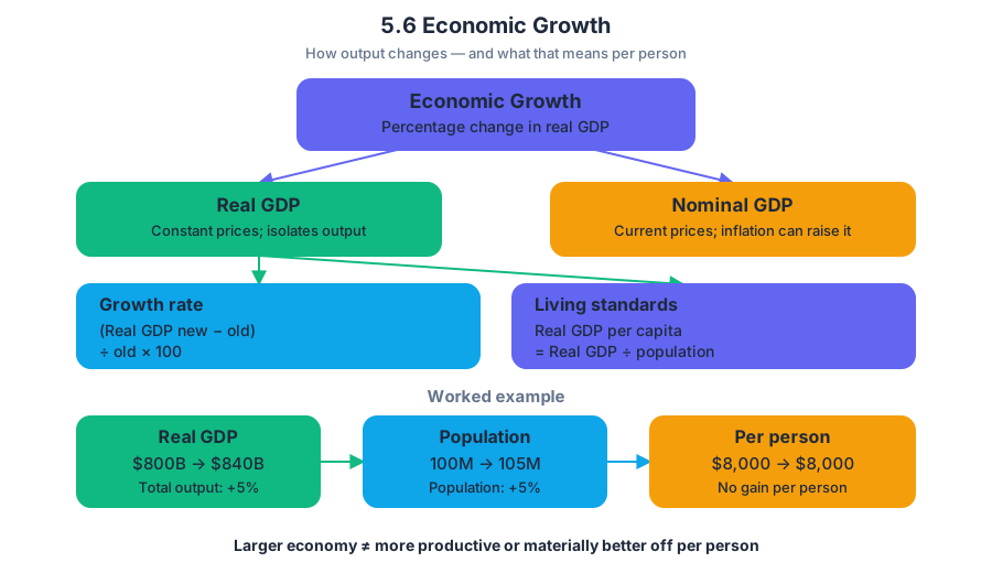
5.7 Public Policy and Economic Growth
Key concepts: Public policy · Productivity · Labor force · Economic incentives · Household economic behavior · Business economic behavior · Long-run economic growth · Government spending · Interest rates · Previously issued bond prices
Public policy can raise long-run economic growth when it changes the incentives that guide household and business decisions, increasing productivity or labor force participation. The central question is not merely “How much does the government spend?” but “How does the policy change the economy’s ability and…
5.7 Public Policy and Economic Growth
Public policy can raise long-run economic growth when it changes the incentives that guide household and business decisions, increasing productivity or labor force participation. The central question is not merely “How much does the government spend?” but “How does the policy change the economy’s ability and willingness to produce?”
POL-4.A.1: Public policies that impact productivity and labor force participation affect real GDP per capita and economic growth.
From incentives to growth
An economic incentive is a reward or cost that influences a decision. A tax credit for job training may encourage firms to invest in worker skills; an earned-income tax credit may increase the incentive for people to work; improved transportation or public education may make productive employment easier. These policies affect behavior first, then productivity or the labor force, and finally the economy’s long-run productive capacity.
The causal chain is:
- Policy changes an incentive
$\rightarrow$ households or businesses alter behavior
$\rightarrow$ labor force participation or productivity changes
$\rightarrow$ potential output and real GDP per capita change
$\rightarrow$ long-run economic growth changes.
Household and business responses
Household economic behavior includes decisions about working, acquiring education, saving, and consuming. For example, a policy that lowers the effective cost of attending technical school can increase human capital. More skilled workers can produce more output per hour, so productivity rises.
Business economic behavior includes decisions about hiring, investment, research, and production methods. A tax incentive for purchasing advanced equipment can reduce the cost of capital. Firms may then invest more, allowing each worker to produce more output. In the long run, this shifts the economy’s productive capacity outward rather than merely increasing demand temporarily.
A policy can also create a disincentive. If an additional dollar earned causes a household to lose more than a dollar in benefits and pay additional taxes, the effective reward from working may fall. Labor force participation may decrease, reducing the amount of labor available for production.
Supply-side fiscal policy
Supply-side fiscal policies are changes in government spending, taxes, or transfers intended to increase the economy’s productive capacity by affecting incentives, productivity, or labor force participation. Their long-run effect depends on how households and firms respond—not simply on the policy’s label.
For example, suppose a government offers firms a credit equal to $20%$ of eligible research spending. If firms respond by developing more efficient production technology, productivity rises. The result is greater potential real GDP and a higher level of real GDP per capita, assuming population does not increase faster than output.
Government spending: demand now, capacity later
A change in government spending can be represented in the aggregate demand–aggregate supply model. Holding other components constant, an increase in government purchases raises aggregate demand because:
$$AD = C + I + G + NX$$
In the short run, higher government spending shifts $AD$ to the right. Real output and the price level rise at the new short-run equilibrium. If the spending funds infrastructure, education, or research that improves productivity, the policy may also shift long-run aggregate supply or LRAS to the right over time.
The distinction matters:
| Policy effect | Immediate model consequence | Possible long-run consequence |
|---|---|---|
| Government purchases of ordinary goods and services | $AD$ shifts right | Mainly higher short-run output and price level |
| Investment in infrastructure, education, or technology | $AD$ shifts right | Greater productivity and an increase in potential output |
| Tax or transfer change that alters work incentives | Consumption or labor decisions change | Labor force participation and productive capacity may change |
Interest rates and investment incentives
Interest rates connect stabilization policy to long-run growth. A lower interest rate reduces the cost of borrowing, which can encourage businesses to purchase capital and households to finance durable goods or education. Greater business investment can expand the economy’s capital stock and raise future productivity.
The financial mechanism also includes asset prices: when market interest rates rise, the prices of previously issued fixed-payment bonds decrease because new bonds offer higher returns. For growth analysis, the key real-economy channel is that higher borrowing costs tend to discourage interest-sensitive investment, while lower borrowing costs can increase investment and support a higher future level of productive capacity.
Misconception check
Misconception: “Every increase in government spending causes economic growth.” Government spending can raise $AD$ and short-run real GDP without increasing productivity. Long-run growth requires a lasting increase in productive capacity—such as better technology, more human capital, a larger participating labor force, or a greater capital stock.
Retrieval check
A government increases spending on a nationwide broadband network and gives firms a tax credit for worker training. Identify one household or business incentive, state the likely effect on productivity or labor force participation, and describe the long-run consequence. Then state what happens to $AD$ immediately if government purchases increase.
Answer: The training credit lowers firms’ cost of improving worker skills, so productivity may rise. The broadband investment immediately shifts $AD$ right and may later increase productive capacity, raising potential output and long-run real GDP per capita.

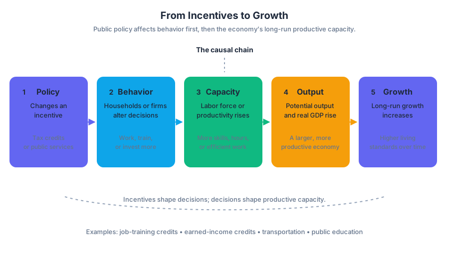
6.1 Balance of Payments Accounts
Key concepts: Capital and financial account (CFA) · Financial capital transfers between countries · International purchases and sales of assets · Balance of payments identity · Current account (CA) deficit · CFA surplus · Currency depreciation · Changes in the value of a currency · Exchange-rate effects on imports
A country can buy more from the world than it sells and still “pay” for the difference—because foreign investors may purchase its assets. The balance of payments (BOP) records these international transactions and explains why a trade imbalance is matched by a financial flow.
6.1 Balance of Payments Accounts
A country can buy more from the world than it sells and still “pay” for the difference—because foreign investors may purchase its assets. The balance of payments (BOP) records these international transactions and explains why a trade imbalance is matched by a financial flow.
Balance of payments: an accounting system that records a country’s international transactions during a particular time period. It consists of the current account (CA) and the capital and financial account (CFA). (MEA-4.A.5)
The two accounts that must fit together
The current account (CA) records transactions involving currently produced goods and services, including net exports, where $NX = X - M$. The capital and financial account (CFA) records financial capital transfers between countries and international purchases and sales of assets such as stocks, bonds, factories, and real estate. (MEA-4.A.2, MEA-4.A.3)
The CFA may show either a surplus, meaning a net financial-capital inflow, or a deficit, meaning a net financial-capital outflow. The capital account and financial account should not be treated as two entirely separate balances when applying the AP relationship: the relevant combined measure is the capital and financial account (CFA). (MEA-4.A.4)
For accounting purposes, the two accounts offset one another:
$$CA + CFA = 0$$
This identity means that a current-account deficit corresponds to an offsetting CFA surplus. If a country imports more goods and services than it exports, the money flowing out through the CA is matched by financial capital flowing into the country through foreign purchases of domestic assets.
| Account movement | Meaning | Required counterpart |
|---|---|---|
| $CA < 0$ | Current-account deficit | $CFA > 0$, a CFA surplus |
| $CA > 0$ | Current-account surplus | $CFA < 0$, a CFA deficit |
| $CA = 0$ | Current account balances | $CFA = 0$ |
Worked example: a current-account deficit
Suppose Country A imports $120$ billion of goods and services but exports only $90$ billion. Its net exports are:
$$NX = X - M = 90 - 120 = -30$$
Assume this makes the current account equal to $-30$ billion. To keep the BOP in balance:
$$CA + CFA = 0$$
$$-30 + CFA = 0$$
$$CFA = 30$$
Country A therefore has a CFA surplus of $30$ billion. Foreign investors must be purchasing $30$ billion more of Country A’s assets than Country A’s residents are purchasing of foreign assets. The deficit does not mean the country’s accounts are “broken”; it identifies the financial inflow financing the current-account deficit.
Why direction matters: Jamaica
A depreciation means that the Jamaican dollar falls in value relative to another currency. The direction must be stated explicitly: writing only “the Jamaican dollar changes” is incomplete, and saying it appreciates when it actually depreciates reverses the economic result.
Exchange-rate changes can also affect the value of imports. For example, if the Jamaican dollar depreciates against the U.S. dollar, U.S. goods become more expensive when priced in Jamaican dollars. Even if the physical quantity of U.S. imports does not immediately change, their measured value in Jamaican currency can increase.
Common misconception: “a deficit means no investment”
Misconception check — “A current-account deficit means financial capital leaves the country.” The opposite is true under the BOP identity. A CA deficit is paired with a CFA surplus: money spent on net imports flows outward, while foreign financial capital flows inward to purchase domestic assets.
AP reasoning process — Principles and Models: Use the accounting model rather than an isolated verbal rule. Identify the sign of the CA, substitute it into $CA + CFA = 0$, and infer the opposite sign for the CFA. This is the complete causal-and-accounting chain exam scoring rewards.
Retrieval check
A country records a current-account deficit of $-45$ billion. What must its CFA equal, assuming the accounts balance? State the result in words as well as symbols.
Answer: $CFA = +45$ billion, so the country has a CFA surplus, representing a net financial-capital inflow.
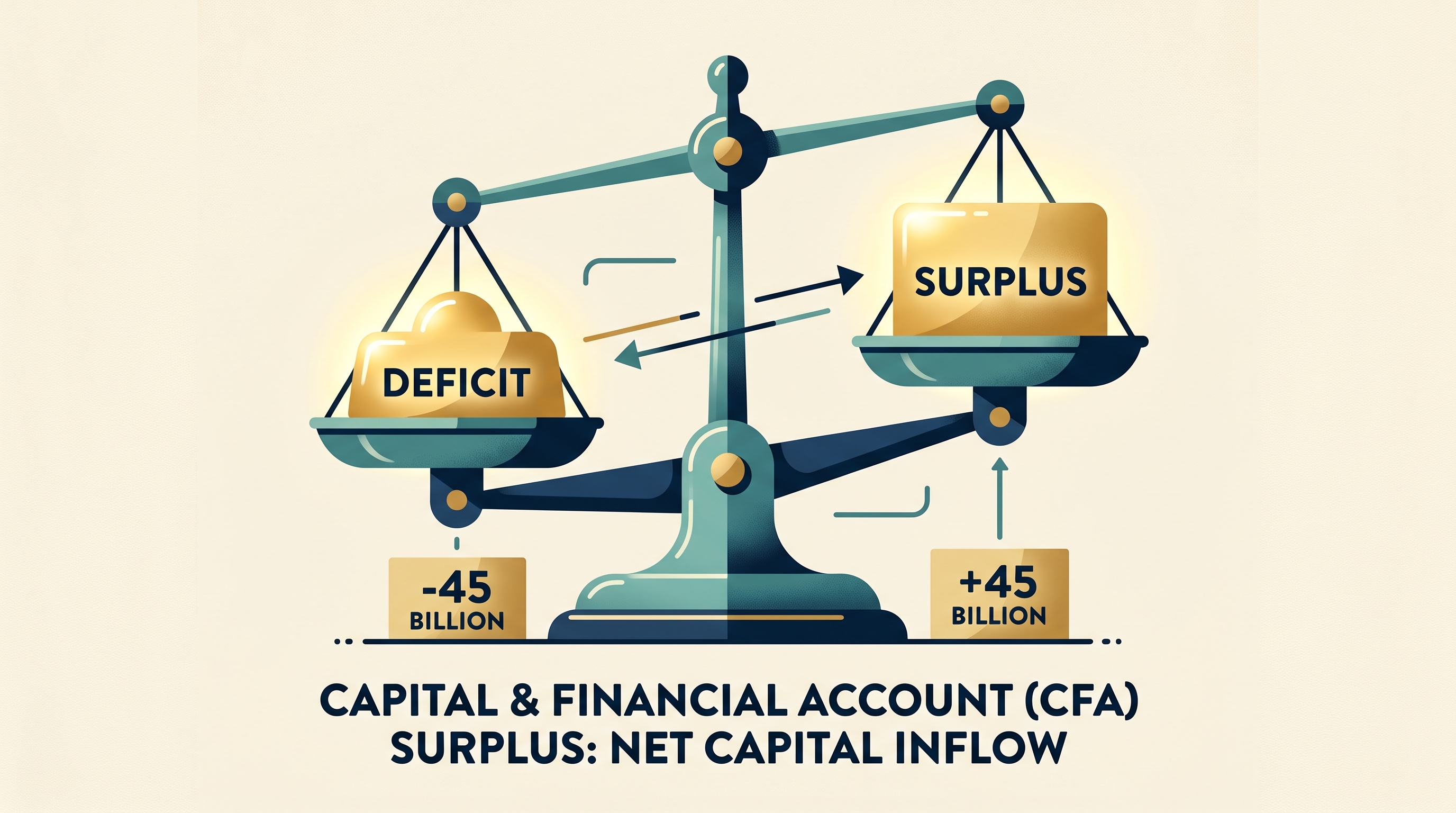
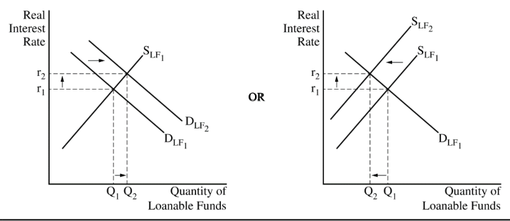
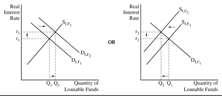
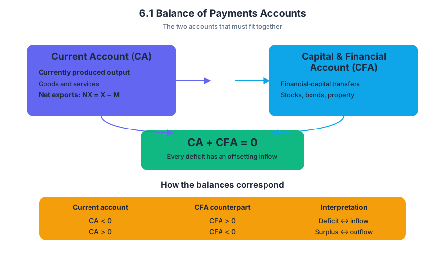
6.2 Exchange Rates
An exchange rate is the price of one currency measured in units of another currency. If $1$ U.S. dollar exchanges for €$0.92$, then the exchange rate is $0.92$ euros per dollar: $1\ \text{USD} = €0.92$.
6.2 Exchange Rates
An exchange rate is the price of one currency measured in units of another currency. If $1$ U.S. dollar exchanges for €$0.92$, then the exchange rate is $0.92$ euros per dollar: $1\ \text{USD} = €0.92$.
The key question is always: which currency is being priced, and which currency is the unit of measurement? A quotation such as €/$ means “euros per dollar,” while $/€ means “dollars per euro.” These are reciprocals:
$$ \text{€ per $}=\frac{1}{\text{$ per €}} $$
If $1$ dollar equals €$0.92$, then $1$ euro equals approximately $1.09$ dollars:
$$ \frac{1}{0.92}\approx 1.09 $$
Appreciation and depreciation
A currency appreciates when it becomes more valuable relative to another currency. It can then purchase more units of the foreign currency. A currency depreciates when it becomes less valuable and purchases fewer units of the foreign currency.
Suppose the exchange rate changes from $1\ \text{USD}=€0.92$ to $1\ \text{USD}=€0.80$. One dollar now buys fewer euros, so the dollar has depreciated relative to the euro. Equivalently, the euro has appreciated relative to the dollar.
The direction depends on the quotation. If the exchange rate is written as dollars per euro, $1\ \text{EUR}=$1.09$ becoming $1\ \text{EUR}=$1.25$ means the euro appreciates. But if it is written as euros per dollar, €/$, an increase means the dollar appreciates relative to the euro. Never label appreciation or depreciation until the numerator and denominator currencies are clear.
Exam rule: An increase in a currency’s value is an appreciation; a decrease is a depreciation. The numerical direction alone is not enough.
Worked contextual example: travel and trade
A U.S. student plans to buy a €$500$ camera. Initially, the exchange rate is $1\ \text{USD}=€0.92$. The dollar cost is:
$$ \text{Cost in dollars}=\frac{€500}{€0.92/$1}\approx $543.48 $$
Now suppose the dollar appreciates to $1\ \text{USD}=€1.00$. The same camera costs:
$$ \frac{€500}{€1.00/$1}=$500 $$
The appreciated dollar makes European goods cheaper for U.S. buyers. At the same time, U.S. goods become more expensive to European buyers because each euro purchases fewer dollars. Thus, holding other factors constant:
- U.S. imports tend to increase.
- U.S. exports tend to decrease.
- U.S. net exports, defined as $NX=X-M$, tend to decrease.
The reverse occurs after a dollar depreciation: U.S. exports become relatively cheaper to foreign buyers, imports become relatively more expensive to U.S. buyers, and U.S. net exports tend to increase. The effect on aggregate demand follows because net exports are one component of aggregate demand:
$$ AD=C+I+G+NX $$
Connection to international accounts
An exchange-rate movement also changes the value of international transactions when they are converted into a common currency. A U.S. firm earning revenue in euros receives fewer dollars when the dollar appreciates, even if the euro price of the product has not changed. This is why exchange rates matter for both trade decisions and the recording of international flows.
Common misconception: “a higher number always means appreciation”
Misconception: “If the exchange-rate number rises, the domestic currency must have appreciated.”
Correction: The quotation determines the interpretation. If the rate rises from $$1.10$ per euro to $$1.25$ per euro, the euro appreciates because it now costs more dollars. But if the rate rises from €$0.91$ per dollar to €$0.95$ per dollar, the dollar appreciates because it now buys more euros.
AP reasoning and skills
This topic is assessed through Learning Objective 6.2.A: Define exchange rates and the associated Essential Knowledge 6.2.A.1: An exchange rate is the price of one currency in terms of another currency. Apply the identifiers by naming both currencies, identifying the quotation, and then explaining the appreciation or depreciation rather than guessing from the number.
The most important connected AP skills are Skill Category 1: Principles and Models, especially 1.A: Define economic principles and models and 1.B: Explain economic principles and models; Skill Category 2: Interpretation, especially 2.A: Identify economic concepts, principles, and models and 2.B: Interpret economic data, information, and models; Skill Category 3: Manipulation, especially 3.A: Solve economic problems using mathematical procedures; and Skill Category 4: Graphing and Visuals, especially 4.A: Draw correctly labeled graphs and visual representations. In practice, these skills require students to interpret a currency quotation, calculate a reciprocal or converted price, and connect the exchange-rate change to exports, imports, and net exports.
Retrieval check: If the exchange rate changes from $$1=€0.80$ to $$1=€0.88$, which currency appreciated? What happens to the dollar price of a €$440$ product?
Answer: The dollar appreciated because it buys more euros. The product’s dollar price falls from $$550$ to $$500$:
$$ \frac{€440}{€0.80/$1}=$550, \qquad \frac{€440}{€0.88/$1}=$500 $$
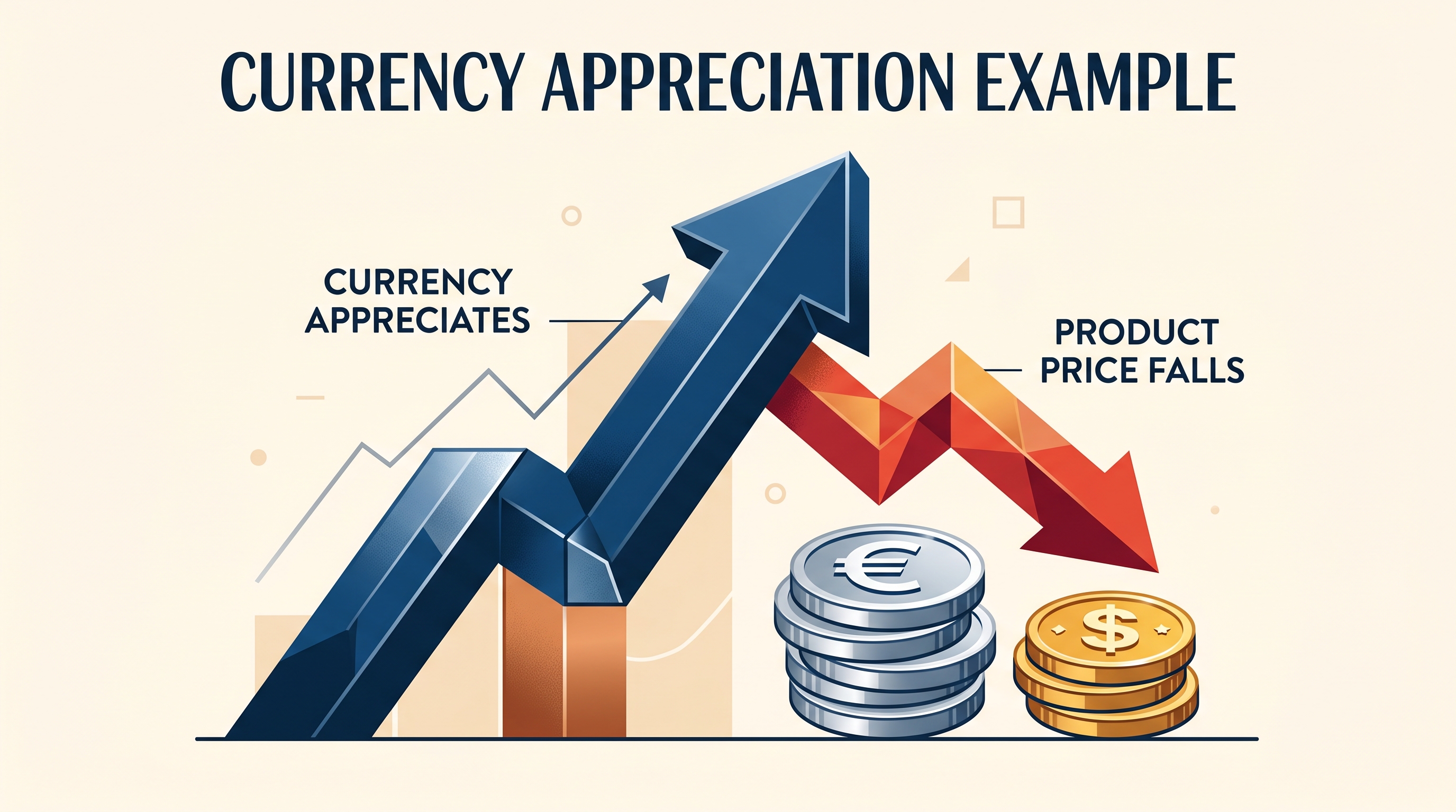
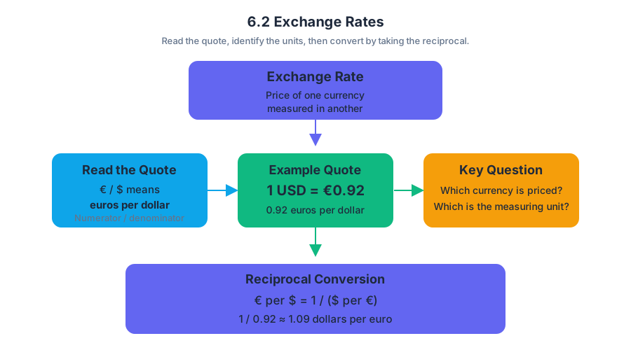
6.3 The Foreign Exchange Market
Key concepts: Foreign exchange market · Exchange rate · Currency appreciation · Currency depreciation · Equilibrium exchange rate · Supply and demand for currency · Flexible exchange market · International trade and financial capital flows · Balance of payments (BOP) · Currency valuation
The foreign exchange market is where buyers and sellers trade one country’s currency for another. Its central question is simple: when millions of international payments and investments occur, what determines the price of a currency?
6.3 The Foreign Exchange Market
The foreign exchange market is where buyers and sellers trade one country’s currency for another. Its central question is simple: when millions of international payments and investments occur, what determines the price of a currency?
Use the exchange-rate convention established in Topic 6.2. For a market for euros priced in U.S. dollars, the vertical axis records dollars per euro, and the horizontal axis records the quantity of euros traded. A quote of $1.20 per euro means that $60 exchanges for $50 euros; the important point here is how buyers and sellers create that market price.
Currency flows create demand and supply
International trade and international finance send currencies in opposite directions. When U.S. residents buy European goods, services, or financial assets, they need euros. Their purchases create demand for euros. When European residents buy U.S. goods, services, or assets, they need dollars; to obtain those dollars, they supply euros in the foreign exchange market.
The same logic applies to financial capital. If investors purchase foreign stocks, bonds, factories, or other assets, they first exchange their domestic currency for the currency in which the asset is priced. Thus, currency demand can arise from demand for a country’s goods, services, and financial assets, while currency supply arises from making payments in other currencies.
MKT-5.B.1: The demand for a currency in a foreign exchange market arises from the demand for the country’s goods, services, and financial assets and shows the inverse relationship between the exchange rate and the quantity demanded of a currency.
MKT-5.B.2: The supply of a currency in a foreign exchange market arises from making payments in other currencies and shows the positive relationship between the exchange rate and the quantity supplied of a currency.
Reading the foreign exchange graph
In the euro market, the demand curve slopes downward. When the dollar price of a euro rises, European goods, services, and assets become more expensive for U.S. buyers, so the quantity of euros demanded decreases. When the dollar price of a euro falls, those purchases become relatively cheaper, so the quantity of euros demanded increases.
The supply curve for euros slopes upward. A higher dollar price per euro gives euro holders more dollars in exchange for each euro, encouraging them to supply more euros to purchase U.S. goods, services, and assets. Therefore, the exchange rate and the quantity supplied of a currency have a positive relationship.
A correctly labeled graph should identify:
- the vertical axis as the exchange rate, such as dollars per euro;
- the horizontal axis as the quantity of euros;
- a downward-sloping demand curve, $D_{\text{€}}$;
- an upward-sloping supply curve, $S_{\text{€}}$; and
- the equilibrium point where the two curves intersect.
Equilibrium, appreciation, and depreciation
The equilibrium exchange rate is the price at which the quantity of a currency demanded equals the quantity supplied. At this point, currency buyers can complete their desired purchases, and currency sellers can complete their desired sales.
MKT-5.C: The equilibrium exchange rate is determined where the quantity demanded and quantity supplied of a currency are equal.
If demand for euros increases while supply is unchanged, the euro’s dollar price rises. The euro appreciates, meaning its value increases relative to the dollar. If demand for euros decreases, the euro’s dollar price falls and the euro depreciates.
Because currencies are always valued relative to one another, one currency’s appreciation is simultaneously the other currency’s depreciation. If the euro appreciates against the dollar, fewer dollars are needed to purchase a given amount of European goods in euro terms, while European buyers find U.S. goods relatively more expensive in their own currency.
Worked market example
Suppose U.S. households begin purchasing more European streaming subscriptions and European investors purchase more U.S. corporate assets. The first transaction increases demand for euros; the second supplies euros because European investors exchange euros for dollars. On a euro foreign-exchange graph, demand shifts right and supply shifts right. The new equilibrium exchange rate depends on the relative size of the two shifts—not on the fact that “more international activity” automatically raises or lowers the euro’s value.
This market therefore coordinates two-way flows: trade moves currencies because buyers pay for imports and sellers receive payment for exports, while capital moves currencies because investors exchange funds to acquire foreign assets. Changes in the equilibrium exchange rate then alter the relative prices of traded goods, services, and assets across countries.
Misconception check
Misconception: “A country supplies its own currency when it exports.” In the foreign exchange market for euros, a U.S. export to Europe creates demand for dollars and supply of euros by the European buyer. Always identify which currency is on the horizontal axis and ask who needs that currency to complete a purchase.
Retrieval check
In a market for Malaysian ringgit priced in Japanese yen, Japanese firms purchase more Malaysian services. Which curve shifts, and what happens to the ringgit?
Answer: Demand for ringgit shifts right because Japanese firms need ringgit to pay Malaysian sellers. The equilibrium quantity of ringgit rises, and the ringgit appreciates relative to the yen if supply does not change. This application uses 3.B: Manipulation, determining the effect of a change in one economic market on another, and 4.A: Graphing, representing the foreign exchange market with correctly labeled axes, curves, and equilibrium.
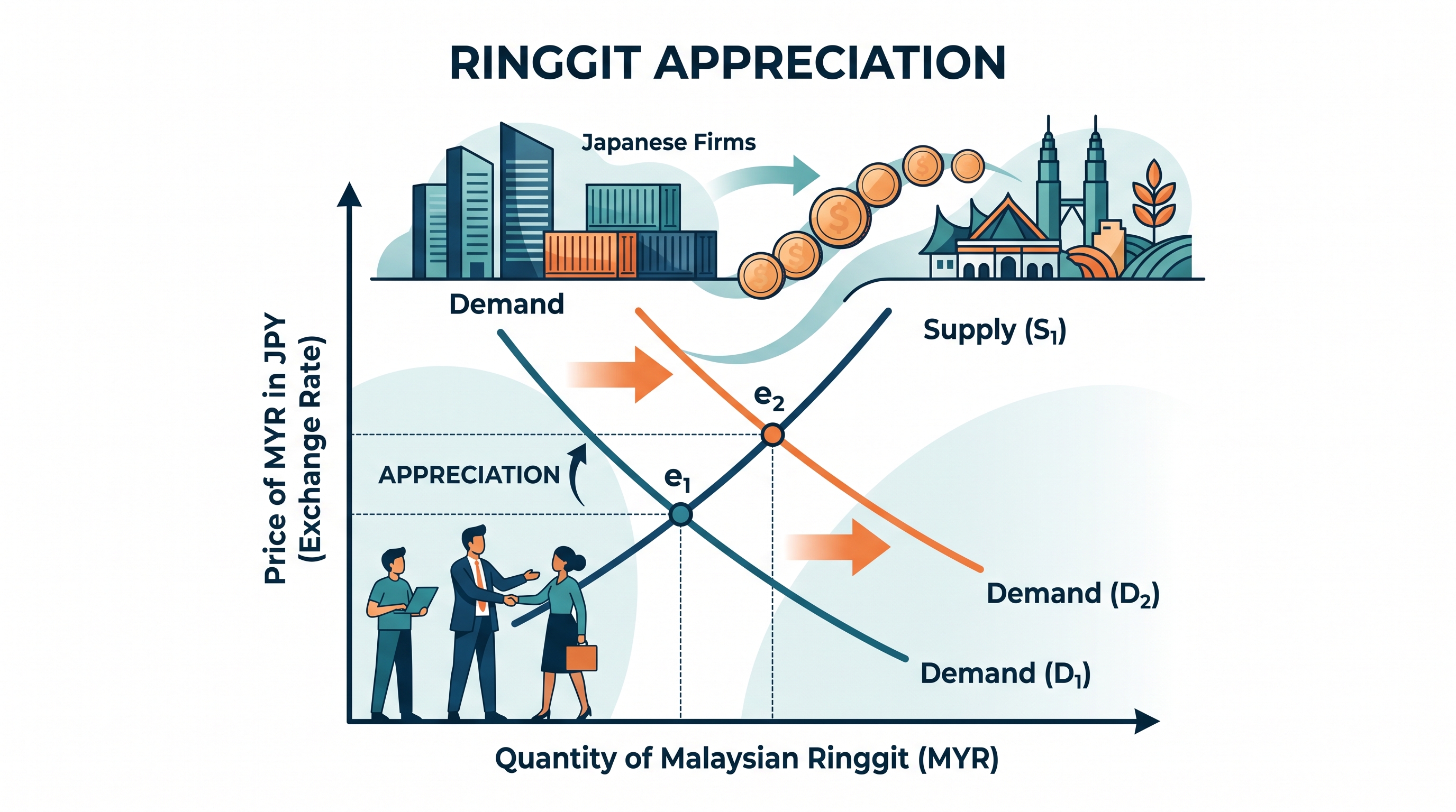
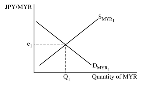
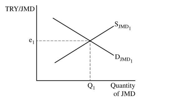
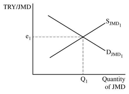
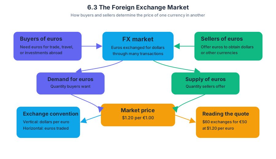
6.4 Effects of Changes in Policies and Economic Conditions on the Foreign Exchange Market
Key concepts: Supply-and-demand models in different market contexts · Macroeconomic graphs as tools for analyzing economic situations · Production possibilities curve (PPC) · Economic growth and full-employment output · Labor force participation rate · Unemployment rate · Full employment · Frictional and structural unemployment · Natural rate of unemployment · Business cycle phases and turning points
A policy change can move a currency even when the foreign-exchange market itself has not changed its basic structure: investors simply alter which assets they want to hold, and buyers or sellers of the currency respond.
6.4 Effects of Changes in Policies and Economic Conditions on the Foreign Exchange Market
A policy change can move a currency even when the foreign-exchange market itself has not changed its basic structure: investors simply alter which assets they want to hold, and buyers or sellers of the currency respond. Using the market model from 6.3 as a working reference, the key task is to identify whether an event changes the demand for the currency or the supply of the currency, then trace the resulting exchange-rate movement.
Policy changes and currency demand or supply
Suppose a central bank adopts expansionary monetary policy by lowering interest rates. Domestic financial assets become less attractive relative to foreign assets, so investors move funds abroad. To purchase foreign assets, they sell the domestic currency; this increases the currency’s supply in the foreign-exchange market and tends to depreciate its value.
The reverse occurs with contractionary monetary policy. Higher domestic interest rates can attract foreign financial capital because investors seek the country’s now-higher returns. Foreign investors must buy the domestic currency to purchase domestic assets, increasing demand for that currency and tending to cause appreciation.
A complete causal chain is more valuable than a one-word answer:
$$ \text{contractionary monetary policy} \rightarrow \text{higher interest rates} \rightarrow \text{greater capital inflows} \rightarrow \text{higher demand for domestic currency} \rightarrow \text{currency appreciation} $$
For example, if Zeetoland’s central bank raises an administered interest rate to fight inflation in an ample-reserves system, investors may purchase more Zeetoland assets. On a graph of the foreign-exchange market for the zeet, the demand curve for zeets shifts right. The equilibrium exchange rate rises, meaning the zeet appreciates.
Other economic conditions
Economic growth can also affect currency markets. Growth expands productive capacity, represented by an outward shift of the production possibilities curve (PPC). If growth makes domestic firms and assets more attractive, foreign investors may demand more of the domestic currency. A stronger currency can then influence international transactions, although the exact effect on exports and imports is analyzed separately through net exports.
Macroeconomic graphs are not illustrations added after the reasoning; they are models that show the mechanism. A correctly drawn foreign-exchange graph must show the currency on the horizontal axis, the exchange rate on the vertical axis, the original and new curve when a shift occurs, and arrows indicating the direction of the shift. The written explanation must connect the shift to its cause.
Graphing rule: Do not shift a curve merely because the exchange rate changes. Shift the curve because an underlying determinant—such as interest rates, capital flows, or economic conditions—changes.
Full employment, output, and labor-market statistics
Full-employment real output is the amount of real output produced when the economy is at full employment. “Full employment” does not mean that every adult has a job; it means unemployment equals the natural rate of unemployment, which consists of frictional and structural unemployment:
$$u_N = u_F + u_S$$
The natural rate excludes cyclical unemployment. When actual unemployment is above the natural rate, the economy generally has an employment shortfall and produces below full-employment output. When actual unemployment is below the natural rate, the economy may be producing beyond its sustainable full-employment level, creating an inflationary gap.
The labor-force statistics require careful classification. The labor force includes employed people and unemployed people who are actively seeking work. A full-time worker and a part-time worker are both employed; neither is counted as unemployed merely because the person works fewer than standard full-time hours.
$$\text{Labor force participation rate} = \frac{\text{Labor force}}{\text{Adult population}} \times 100$$
$$\text{Unemployment rate} = \frac{\text{Unemployed people}}{\text{Labor force}} \times 100$$
Worked example. An economy has an adult population of $1{,}000$, with $620$ employed full-time, $80$ employed part-time, $50$ unemployed and actively seeking work, and $250$ outside the labor force.
$$\text{Labor force}=620+80+50=750$$
$$\text{Participation rate}=\frac{750}{1{,}000}\times100=75%$$
$$\text{Unemployment rate}=\frac{50}{750}\times100\approx6.7%$$
The $250$ people outside the labor force do not enter the unemployment-rate denominator. Someone who has stopped searching for work is not classified as unemployed in the household survey, even though that person may still face economic hardship.
Misconception check: The unemployment rate is not unemployed people divided by the adult population. Its denominator is the labor force.
Business-cycle interpretation
Business cycles are fluctuations in aggregate output and employment caused by changes in aggregate demand and/or aggregate supply (MEA-2.A.1). The two phases are expansion and recession (MEA-2.A.2); the turning points are the peak and trough (MEA-2.A.3).
The difference between actual output and potential output is the output gap (MEA-2.A.4). Potential output is another name for full-employment output: the GDP level at which unemployment equals the natural rate (MEA-2.A.5). Identifying a turning point means locating where output stops rising or falling, not simply noticing that the level of output is high or low.
Retrieval check: A central bank raises interest rates, and foreign investors purchase more domestic assets. Which curve shifts in the foreign-exchange market, and what happens to the currency? Then classify a part-time worker, an active job seeker, and a discouraged nonsearcher for the labor statistics. The answer should be: demand for the domestic currency shifts right and the currency appreciates; the part-time worker is employed, the active job seeker is unemployed, and the discouraged nonsearcher is outside the labor force.
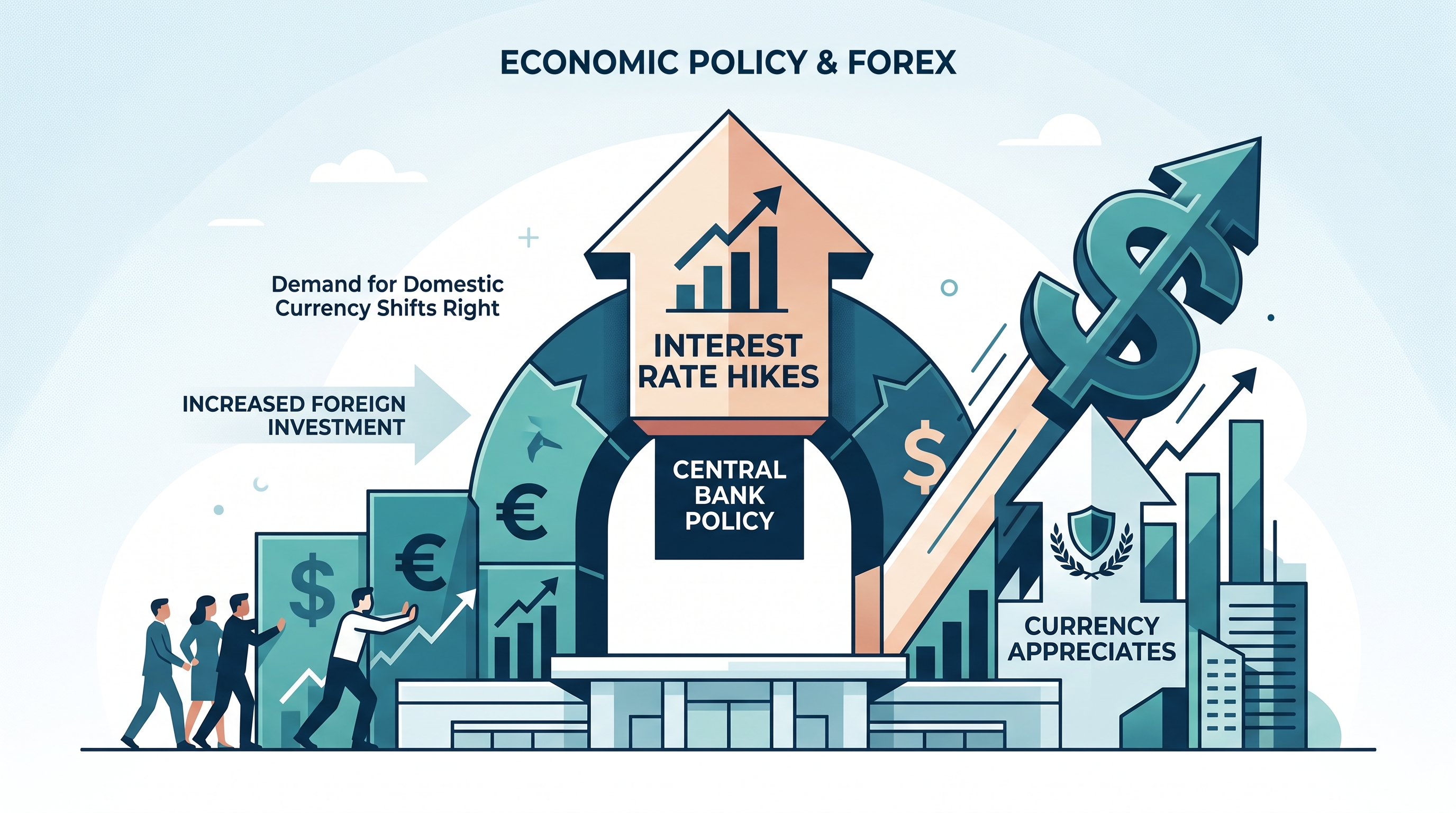
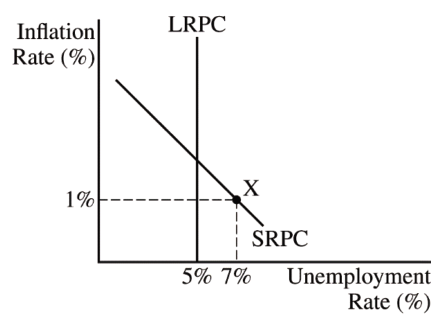
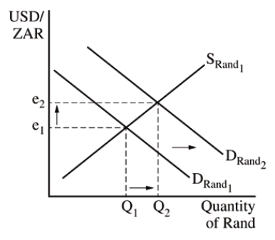
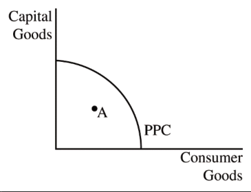
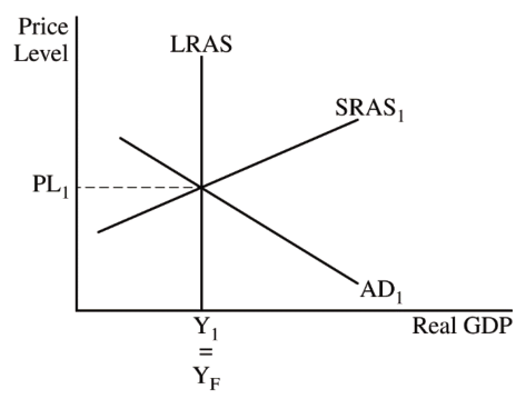
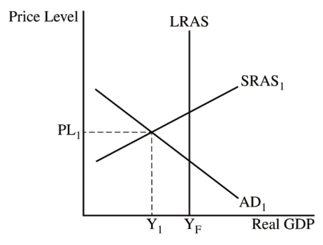
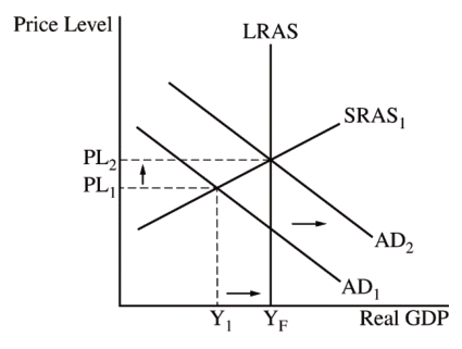
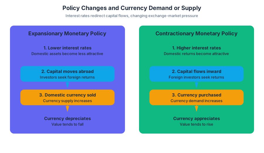
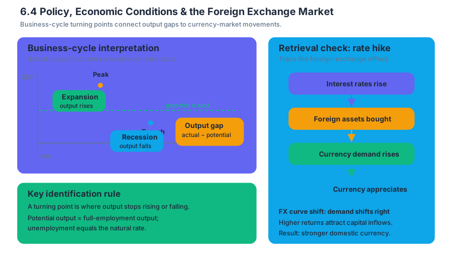
6.5 Changes in the Foreign Exchange Market and Net Exports
Key concepts: Foreign exchange market · Exchange rate · Demand for currency · Supply of currency · Equilibrium exchange rate · Currency appreciation · Currency depreciation · Exports and net exports · Aggregate demand · Foreign trade and current account
An exchange rate is the price of one currency stated in terms of another currency: for example, $0.20 per rand means that one South African rand exchanges for $0.20.
6.5 Changes in the Foreign Exchange Market and Net Exports
An exchange rate is the price of one currency stated in terms of another currency: for example, $0.20 per rand means that one South African rand exchanges for $0.20. In a flexible foreign exchange market, that price changes when the demand for or supply of a currency changes.
MKT-5.E — Currency-market mechanism: Equilibrium occurs where the quantity of a currency demanded equals the quantity supplied, determining the equilibrium exchange rate.
Reading the foreign exchange market
A foreign exchange market is a market in which one nation’s currency is exchanged for another. If residents of the United States demand rand, they give up dollars to obtain rand; simultaneously, South Africa supplies rand in exchange for those dollars. The currency being purchased is represented by the market’s demand curve, while the currency being exchanged away is represented by its supply curve.
For a graph of the market for rand, place the exchange rate of the rand in dollars on the vertical axis and the quantity of rand on the horizontal axis. The demand curve slopes downward: a lower dollar price makes rand less expensive to obtain. The supply curve slopes upward: a higher dollar price gives holders of rand a greater incentive to exchange them for dollars.
The intersection of demand and supply gives the equilibrium exchange rate, $e_1$, and equilibrium quantity, $Q_1$. At that point, the quantity of rand demanded equals the quantity supplied. A price above $e_1$ creates a surplus of rand; a price below $e_1$ creates a shortage.
How shifts change a currency’s value
Changes in market conditions shift a currency’s demand or supply curve. A rightward shift in demand raises both the equilibrium exchange rate and the equilibrium quantity. The currency appreciates, meaning its value increases relative to the other currency.
A leftward shift in supply also raises the currency’s equilibrium exchange rate but reduces the equilibrium quantity. For example, if fewer rand enter the foreign exchange market because South Africa exports fewer goods, the supply of rand shifts left. The rand appreciates: each rand now buys more dollars.
Graphing rule: To show appreciation of the currency on the vertical axis, move the equilibrium exchange rate upward from $e_1$ to $e_2$. To show depreciation, move it downward. Always label both original and new curves, equilibria, exchange rates, and quantities.
A currency depreciation is the opposite change: the currency loses relative value. A rightward supply shift or a leftward demand shift lowers its equilibrium exchange rate. In a correctly labeled graph, the new equilibrium exchange rate is below the original one.
Exchange rates and net exports
A country’s net exports are its exports minus its imports:
$$NX = X - M$$
When a country’s currency appreciates, its goods become more expensive to foreign buyers, so exports tend to decrease. At the same time, foreign goods become less expensive to domestic buyers, so imports tend to increase. Therefore, an appreciation decreases net exports.
When a country’s currency depreciates, domestic goods become less expensive to foreigners and imported goods become more expensive to domestic residents. Exports tend to rise, imports tend to fall, and net exports increase.
MKT-5.F — Net exports and aggregate demand: Because net exports are a component of aggregate demand,
$$AD = C + I + G + NX$$
an increase in net exports shifts aggregate demand right, while a decrease in net exports shifts aggregate demand left.
Worked example: an appreciating rand
Suppose the equilibrium exchange rate initially is $0.20 per rand. Stronger foreign demand for South African products increases demand for rand, shifting the rand-demand curve right. The new exchange rate rises to $0.25 per rand: the rand has appreciated.
At $0.25 per rand, a South African product priced at $100 costs a foreign buyer:
$$\frac{$100}{$0.25\text{ per rand}} = 400\text{ rand}$$
Before appreciation, the same product cost:
$$\frac{$100}{$0.20\text{ per rand}} = 500\text{ rand}$$
The product is now cheaper in rand terms, but from the perspective of a foreign buyer using dollars, South African goods require more dollars per rand. More generally, the appreciation makes domestic goods relatively more expensive to foreigners and imports relatively cheaper to domestic residents. The expected result is lower exports, higher imports, lower net exports, and a leftward shift of aggregate demand.
Common misconception check
Misconception: “A stronger currency always improves the trade balance.” A higher currency value makes imported goods cheaper, but it also makes the country’s exports more expensive to foreigners. In the standard AP macroeconomic model, appreciation decreases net exports; depreciation increases net exports.
Retrieval check: In the market for the Vortanian crown, the supply curve shifts left. What happens to the equilibrium exchange rate, the value of the crown, and Vortania’s net exports?
Answer: The equilibrium exchange rate rises, so the crown appreciates. Vortanian exports become relatively more expensive and imports relatively cheaper, causing net exports to decrease. Net exports are recorded in the current account of foreign-trade accounting; detailed financial-capital flows belong with the separate analysis of international capital movements.
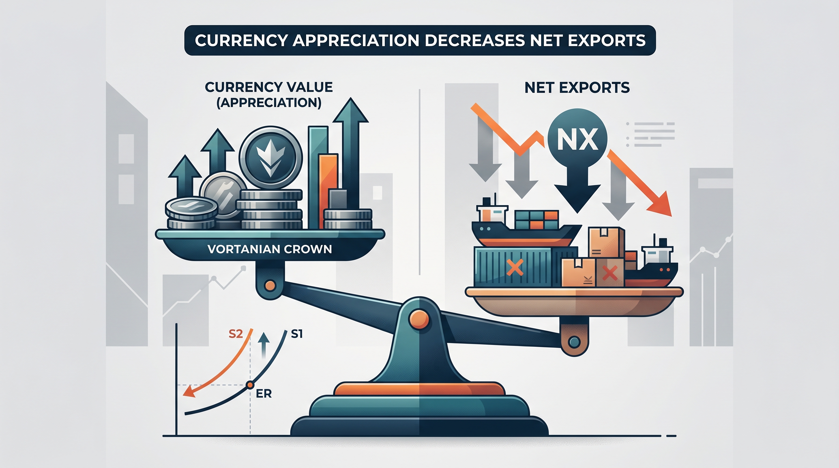
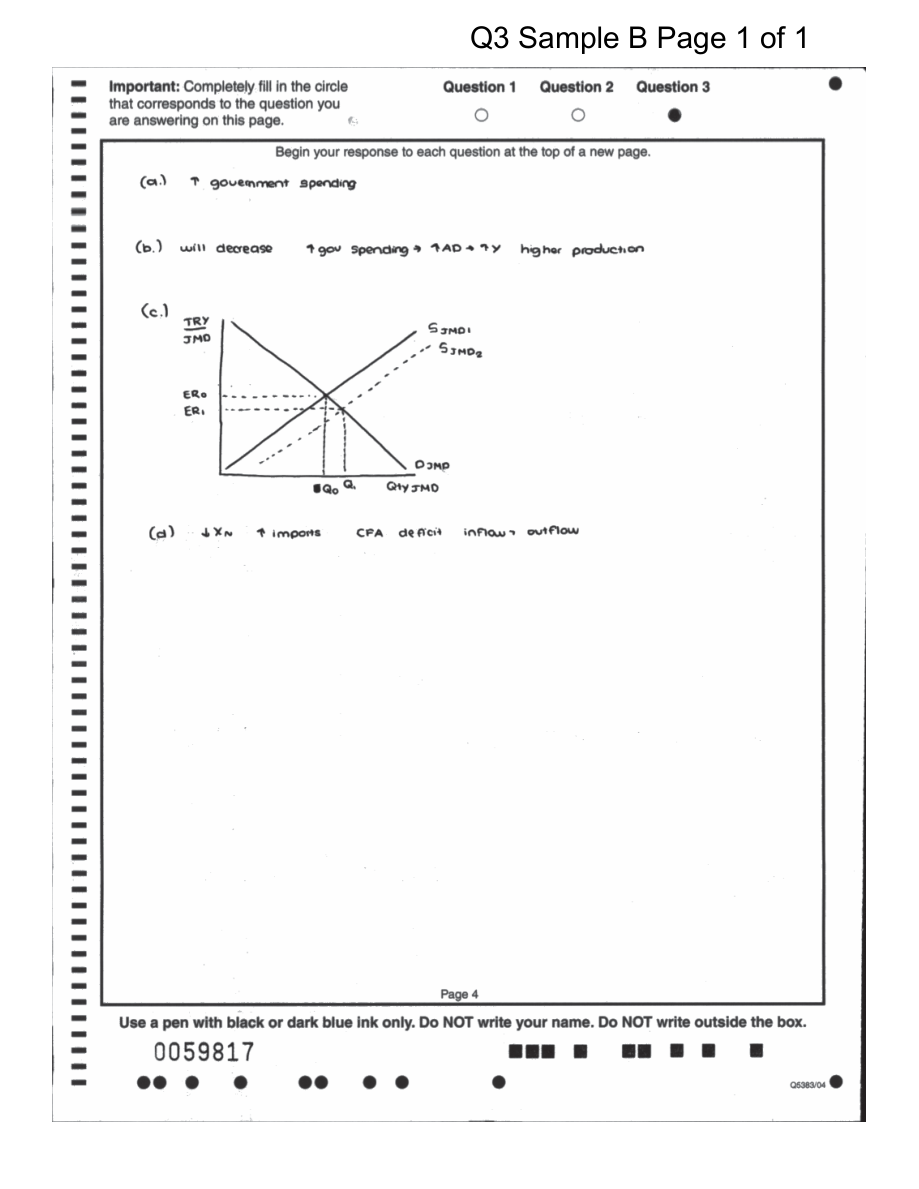
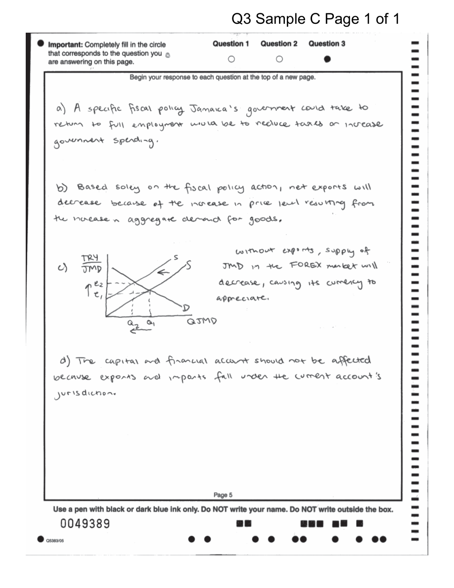
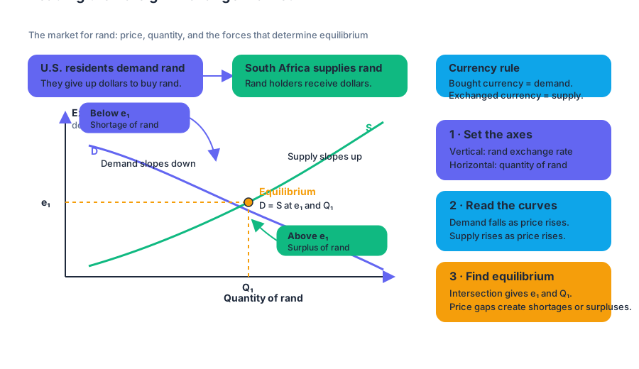
6.6 Real Interest Rates and International Capital Flows
Key concepts: Real interest rates · International capital flows · Exchange rates · Currency appreciation and depreciation · Net exports · Current account · Capital/financial account · Balance of payments · Financial capital inflows and outflows · Interest rates and foreign investment
A saver comparing two countries does not care only about the advertised interest rate; the crucial comparison is the real interest rate, the return after accounting for the purchasing power lost to inflation:
6.6 Real Interest Rates and International Capital Flows
A saver comparing two countries does not care only about the advertised interest rate; the crucial comparison is the real interest rate, the return after accounting for the purchasing power lost to inflation:
$$ \text{Real interest rate} \approx \text{Nominal interest rate} - \text{Actual inflation rate} $$
A bond yielding $7%$ in a country with $4%$ inflation offers an approximate real return of $3%$. If another country offers a nominal rate of $5%$ but has only $1%$ inflation, its real return is approximately $4%$. Financial capital is more likely to move toward the second country, even though its nominal interest rate is lower.
Key distinction: Nominal interest rates measure stated returns in money terms; real interest rates measure approximate gains in purchasing power.
Why real interest-rate differences move capital
International capital flows are movements of money across national borders for investment, trade, or business production. Investors may purchase foreign bonds, firms may build factories abroad, and households or businesses may transfer funds to finance international transactions. Under MKT-5.G.1, differences in real interest rates change the relative attractiveness of domestic and foreign assets.
Suppose Country A’s real interest rate rises above Country B’s. Financial assets in Country A now offer a relatively higher return, so foreign investors demand more of Country A’s assets. The result is a net capital inflow: foreign financial capital entering Country A exceeds domestic financial capital leaving it.
The causal sequence is:
- Country A’s real interest rate rises relative to other countries.
- Country A’s assets become relatively more attractive.
- Foreign investors purchase more Country A assets.
- Country A experiences a net capital inflow.
- Demand for Country A’s currency increases.
- By the exchange-rate mechanism established in Topic 6.5, the currency appreciates and net exports fall.
The important new accounting insight is that the financial inflow is not an isolated event: it is recorded alongside the country’s transactions in the balance of payments.
The balance of payments: two connected accounts
The balance of payments is the accounting system that records a country’s international transactions during a particular period. It consists of the current account and the capital/financial account.
The current account records three broad categories:
- Net exports, or the balance of trade: exports minus imports.
- Income flows, such as interest, profits, and wages received from or paid to other countries.
- Net unilateral transfers, such as foreign aid or remittances that do not purchase a current good or service.
A current-account surplus means the country receives more through these current transactions than it pays out. A current-account deficit means it pays out more than it receives. These definitions correspond to MEA-4.A.1 and MEA-4.A.2.
The capital/financial account records transfers and purchases or sales of assets between countries. A capital/financial account surplus represents a financial capital inflow: foreigners are purchasing more domestic assets than domestic residents are purchasing foreign assets. A capital/financial account deficit represents a financial capital outflow.
| Account | What it records | Surplus means |
|---|---|---|
| Current account | Net exports, income flows, and net unilateral transfers | Net receipts from current international transactions |
| Capital/financial account | International purchases and sales of assets and related capital transfers | Net financial capital inflow |
Because international transactions are recorded from both sides, a country’s current-account balance and capital/financial-account balance move in opposite directions, ignoring statistical discrepancies:
$$ \text{Current account} + \text{Capital/financial account} \approx 0 $$
Thus, a current-account deficit is typically matched by a capital/financial-account surplus. The country is receiving foreign financial capital that helps finance its excess of imports and other current payments over exports and other current receipts.
Worked example: a higher real interest rate
Assume Arandia raises its nominal interest rate from $6%$ to $8%$ while actual inflation remains $2%$. Its approximate real interest rate rises from
$$ 6% - 2% = 4% $$
to
$$ 8% - 2% = 6% $$
If comparable foreign assets still yield a real return of $4%$, Arandian assets become relatively more attractive. Foreign investors purchase Arandian bonds, creating a net capital inflow and a capital/financial account surplus. The increased demand for the Arandian currency causes appreciation, so—through the previously established mechanism—Arandia’s net exports decrease.
If Arandia’s current account consequently records a deficit of $30$ billion, its capital/financial account will show an inflow of approximately $30$ billion, or a surplus of $30$ billion, under the simplified accounting identity. The financial inflow is therefore the counterpart of the current-account deficit, not an unrelated statistic.
Central banks and the international transmission channel
Under MKT-5.G.2, central banks can influence the domestic interest rate in the short run, which changes net capital inflows. A policy that raises domestic interest rates can attract foreign financial capital; a policy that lowers them can reduce that attraction or encourage capital to flow abroad. The comparison is always relative: a domestic rate matters because it is being compared with real returns available in other countries.
Misconception check: “A capital-account surplus is automatically good”
A capital/financial account surplus does not by itself mean an economy is healthier. It means the country is receiving a net inflow of financial capital. That inflow may finance productive investment, but it may also accompany a current-account deficit and greater reliance on foreign financing. Likewise, a current-account deficit is not identical to a government budget deficit; they are different accounts measuring different transactions.
Retrieval check
A country’s nominal interest rate is $9%$ and its actual inflation rate is $6%$, while foreign assets offer a real return of $2%$. What is the country’s approximate real interest rate, and what international financial outcome is most likely?
The real rate is $3%$, so the country’s assets offer the relatively higher return. The likely result is a net capital inflow and a capital/financial account surplus; the currency appreciates and net exports fall through the established foreign-exchange relationship.
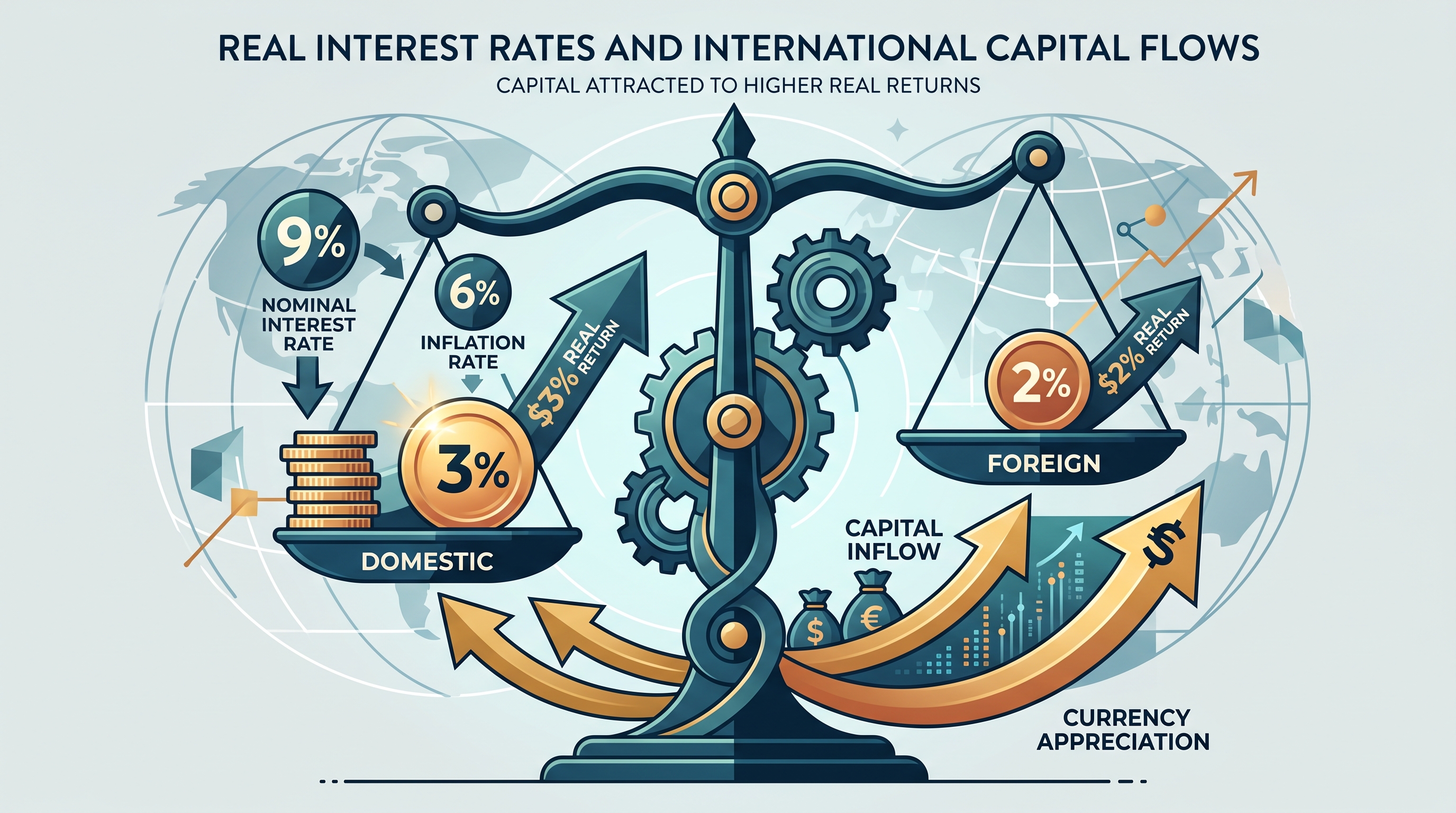
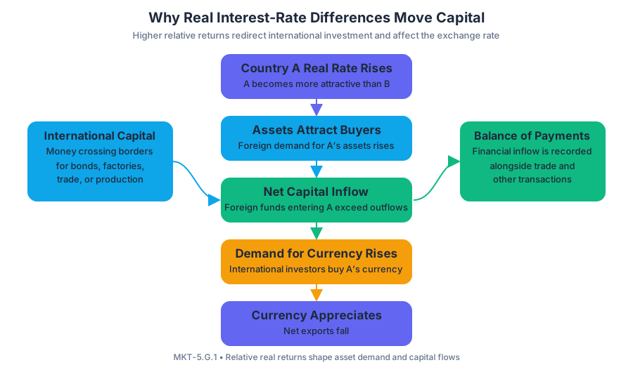
AP Practice 1
Key concepts: AP Macroeconomics course framework · Economic indicators · Business cycle · Economic models · Evidence-based economic analysis · Independent thinking and drawing conclusions · Assessing source credibility · Respectful debate of ideas · College-level coursework readiness · Basic mathematics and graphing skills
AP Macroeconomics asks a deceptively simple question: how can one person’s spending become another person’s income? The answer begins with an economy-wide model. When a household buys a meal, the restaurant receives revenue; the restaurant then pays workers, suppliers, and owners; those recipients spend part of…
AP Practice 1
AP Macroeconomics asks a deceptively simple question: how can one person’s spending become another person’s income? The answer begins with an economy-wide model. When a household buys a meal, the restaurant receives revenue; the restaurant then pays workers, suppliers, and owners; those recipients spend part of that income elsewhere. A single transaction therefore becomes part of a larger circular flow of income and production.
The course’s analytical map
AP Macroeconomics is a college-level, one-semester introduction to the principles governing an economic system as a whole. Its central subjects include economic indicators, such as national income, unemployment, and price levels; the business cycle, which describes fluctuations in economic activity; financial markets; stabilization policies; economic growth; and international economics.
The course is organized around four cross-cutting big ideas:
- MEA: Economic Measurements — using measures such as GDP, unemployment, and inflation to describe economic performance.
- MKT: Markets — explaining how buyers and sellers interact through incentives, prices, and exchange.
- MOD: Macroeconomic Models — using simplified representations, such as the circular-flow model or AD–AS model, to predict and explain outcomes.
- POL: Macroeconomic Policies — analyzing how fiscal and monetary decisions affect the economy.
Economic models are not miniature copies of reality. They deliberately simplify reality so that a particular relationship becomes visible. The circular-flow model emphasizes connections among households, firms, product markets, and factor markets; later models use graphs, equations, charts, and data to isolate different mechanisms. A strong conclusion must therefore identify what the model explains and what it leaves out.
Evidence-based economic analysis
AP students are expected to interpret evidence rather than accept every economic claim at face value. A concise source-evaluation procedure is:
- Author expertise: Does the author or institution have relevant economic or statistical expertise?
- Data provenance: Where did the numbers originate, and can the original dataset or government release be located?
- Methodology: How were variables defined, sampled, measured, or calculated?
- Publication date: Is the evidence current for the question being asked?
- Incentives and conflicts: Could the author, sponsor, firm, or political organization benefit from a particular interpretation?
- Reporting versus opinion: Which statements report measured facts, and which statements are predictions, judgments, or advocacy?
- Corroboration: Do independent, methodologically credible sources support the same conclusion?
Worked source check. Imagine a news article titled “Households Rescue the Economy with a Spending Surge.” The article attributes a reported increase in consumer spending to a national statistical agency. That attribution improves its credibility, but the headline is still interpretation. A careful reader checks the agency’s release, confirms the publication date, determines whether spending is measured in nominal or real terms, examines how the statistic was calculated, and compares the claim with an independent economic analysis. The final conclusion might be narrower than the headline: real consumer spending increased during the measured period and contributed to aggregate demand, but the evidence alone does not prove that households permanently strengthened economic growth.
Key insight: Reliable data do not automatically produce a reliable conclusion; measurement, method, incentives, and interpretation all matter.
Independent thinking does not mean treating every opinion as equally well supported. It means drawing a conclusion that follows from the evidence, stating uncertainty when appropriate, and revising the conclusion when stronger evidence appears. Students are not expected to adopt one cultural or political value system; respectful disagreement is compatible with rigorous economic reasoning, while personal attacks are not.
Original multiple-choice practice
Question — approximately 2 minutes. A researcher observes that nominal household spending rose during a year in which the price level also increased. Which conclusion is most defensible?
A. Households definitely purchased more goods and services in real terms.
B. The economy definitely entered an expansion.
C. Nominal spending increased, but additional evidence is needed to determine whether real consumption increased.
D. The increase in spending proves that inflation was caused by higher household income.
Answer: C. Nominal spending records current-dollar expenditure. Because prices increased, the observed rise may reflect more expensive goods rather than a larger quantity of goods and services purchased. Real spending would require adjusting for the price change. Choices A and B overstate what the evidence establishes; choice D confuses a possible relationship with proof of causation.
For a multiple-choice task, the rewarded reasoning is precise identification of the measured variable, recognition of the model’s limitation, and rejection of conclusions that exceed the evidence. There is no partial credit for an unsupported explanation, so eliminate answers containing words such as definitely when the data do not justify certainty.
Preparation and error review
AP Macroeconomics has no prerequisites. Students should nevertheless be prepared to read a college-level textbook and use basic mathematics and graphing skills. The current exam includes a multiple-choice section and free-response questions; the same habits—defining variables, reading graphs, manipulating relationships, and explaining evidence—support both formats.
After answering, record three things: the variable the question measured, the assumption or limitation you noticed, and the exact word that made each distractor incorrect. If your error was confusing nominal with real values, label it a measurement error; if you accepted the headline without checking its evidence, label it a source-credibility error. That diagnosis is more useful than simply marking the answer wrong.

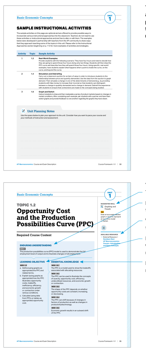



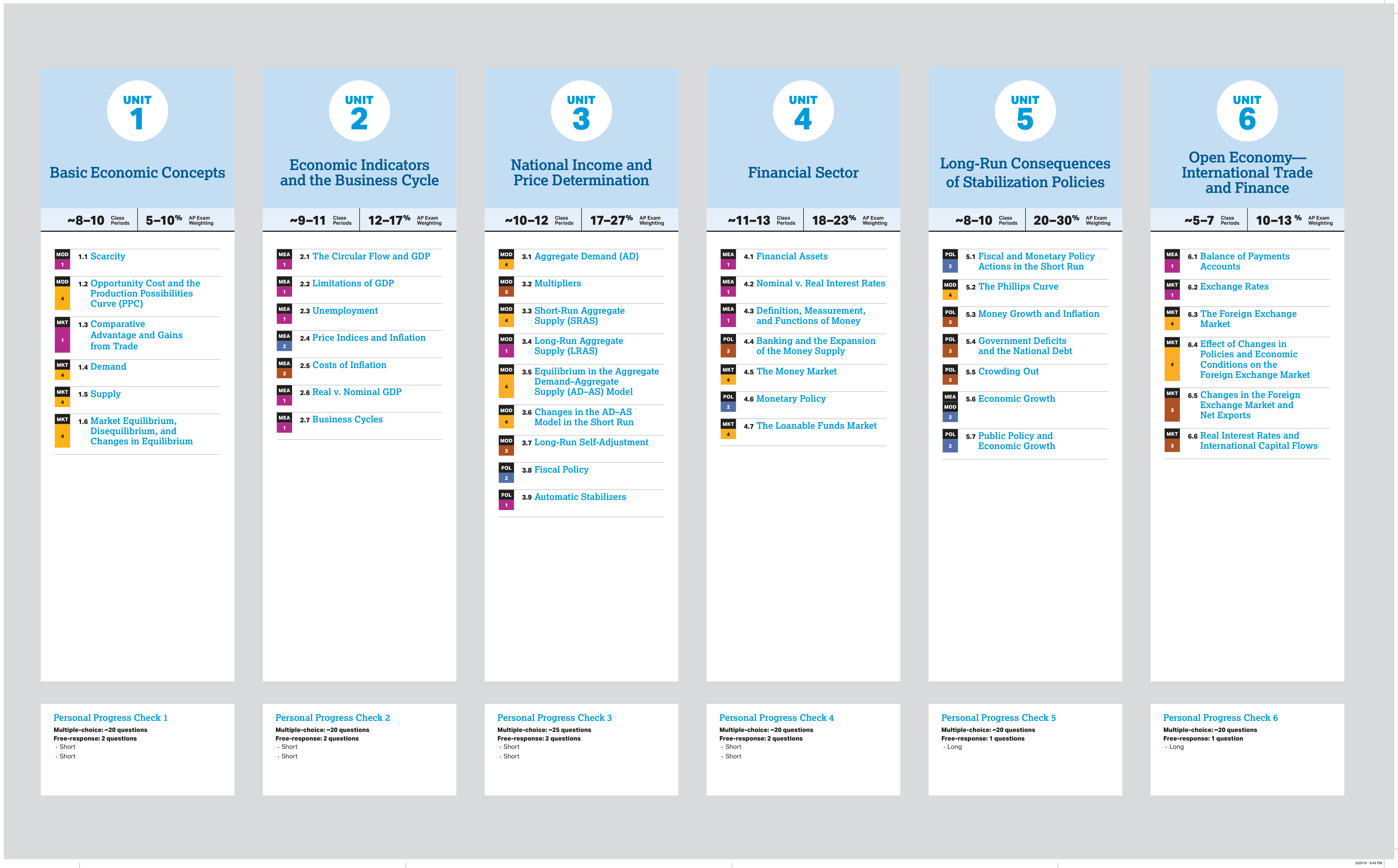

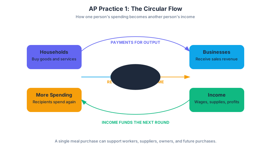
AP Practice 2
Key concepts: International trade and balance of payments · Exports, imports, and net exports · Domestic currency and exchange-rate effects on trade · Unemployment rate · Labor force participation rate · Economic performance indicators, including gross domestic product · Economic growth and contraction · Reserve banking and central-bank policies · Demand and supply graphs, including movements along curves versus shifts · Quantitative analysis and economic calculations
A country can look healthier on one economic indicator while appearing weaker on another: real GDP may grow even as unemployment remains high, and a stronger domestic currency may make imports cheaper while reducing net exports.
AP Practice 2
A country can look healthier on one economic indicator while appearing weaker on another: real GDP may grow even as unemployment remains high, and a stronger domestic currency may make imports cheaper while reducing net exports. The central skill is connecting each measurement to the mechanism behind it rather than treating any single number as a complete diagnosis.
Task type: Original, unofficial short free-response practice. Suggested timing is approximately $12$ minutes. This task emphasizes MEA-1: Principles and Models, MEA-2: Interpretation, MEA-3: Manipulation, and MEA-4: Graphing and Visuals, especially quantitative measurement, causal explanation, and correctly labeled economic models.
Practice scenario: Lydora
Lydora’s domestic currency appreciates after foreign investors purchase more Lydoran financial assets. Before the appreciation, Lydora records exports of $$240$ billion and imports of $$275$ billion. Its adult population is $50$ million: $32$ million people are employed, $3$ million are unemployed and actively seeking work, and $15$ million are not in the labor force.
Part A: Net exports
Define net exports and calculate Lydora’s initial net exports.
Scoring target: Define net exports as exports minus imports.
$$NX = X - M$$
$$NX = $240\text{ billion} - $275\text{ billion} = -$35\text{ billion}$$
Lydora has a trade deficit of $$35$ billion because imports exceed exports. A negative value is not “negative trade”; it means the country purchases more goods and services from abroad than it sells abroad.
Part B: Currency appreciation and trade
Explain why Lydora’s currency appreciation is expected to decrease exports, increase imports, and reduce net exports.
Scoring target: A complete causal chain earns the explanation point:
- Appreciation makes Lydoran goods more expensive to foreign buyers.
- Foreign buyers purchase fewer Lydoran exports.
- Appreciation makes foreign goods cheaper for Lydoran residents.
- Lydoran residents purchase more imports.
- Because $NX = X - M$, lower exports and higher imports reduce net exports.
A common misconception is that an appreciating currency automatically improves the trade balance because the currency is “stronger.” The relevant comparison is not national strength; it is the price of domestic goods relative to foreign goods.
Part C: Labor-market measurements
Calculate Lydora’s labor force, unemployment rate, and labor force participation rate. Show work.
The labor force includes people who are employed plus people who are unemployed and actively seeking work:
$$\text{Labor force} = \text{employed} + \text{unemployed}$$
$$\text{Labor force} = 32 + 3 = 35\text{ million}$$
The unemployment rate is the percentage of the labor force that is unemployed:
$$\text{Unemployment rate} = \frac{\text{unemployed}}{\text{labor force}}\times 100$$
$$\text{Unemployment rate} = \frac{3}{35}\times 100 \approx 8.6%$$
The labor force participation rate is the percentage of the adult population in the labor force:
$$\text{LFPR} = \frac{\text{labor force}}{\text{adult population}}\times 100$$
$$\text{LFPR} = \frac{35}{50}\times 100 = 70%$$
The adult population is broader than the labor force. It includes the $15$ million people outside the labor force, such as retirees, full-time students, and discouraged workers. Because discouraged workers are not actively seeking work, they are excluded from both the labor force and the measured unemployment rate.
Part D: Economic performance
Lydora’s real GDP rises from $$800$ billion to $$824$ billion. Calculate the real GDP growth rate and identify whether the economy experiences growth or contraction.
$$\text{Growth rate} = \frac{\text{new real GDP} - \text{old real GDP}} {\text{old real GDP}}\times 100$$
$$\text{Growth rate} = \frac{824-800}{800}\times 100 = 3%$$
Real GDP rises by $3%$, so Lydora experiences economic growth. A decrease in real GDP would indicate an economic contraction. GDP measures the market value of final goods and services produced within a country, but GDP alone does not measure income distribution, unpaid household production, environmental quality, or every aspect of economic well-being. Inflation and unemployment provide additional evidence about economic performance.
Part E: Reserve banking and policy
Lydora’s central bank purchases government securities from commercial banks. State the immediate effect on bank reserves and identify the likely short-run effect on aggregate demand.
A government-securities purchase increases commercial-bank reserves. In a reserve-banking system, banks can use additional reserves to support more lending, which tends to increase the money supply and lower interest rates. Lower interest rates encourage interest-sensitive consumption and investment, shifting aggregate demand rightward in the short run.
Part F: Curve reasoning and graphing
On a correctly labeled foreign-exchange-market graph for Lydora’s currency, show the effect of increased foreign demand for Lydoran financial assets. Label the vertical axis, horizontal axis, currency-demand curve, currency-supply curve, initial equilibrium, and the new equilibrium.
Scoring target: Put the exchange rate, measured as the price of Lydora’s currency in another currency, on the vertical axis. Put the quantity of Lydora’s currency on the horizontal axis. Increased foreign demand shifts the demand curve right, raising the equilibrium exchange rate and causing appreciation.
This is a shift of the demand curve, not a movement along the original demand curve: the cause is a change in foreign demand for the currency. By contrast, a change in the currency’s own exchange rate would produce a movement along a fixed demand curve.
Error-review routine
After completing the task, mark each missed point as one of four errors: definition, calculation, graph labeling, or causal chain. Rewrite only the missing link. For example, replace “appreciation lowers net exports” with “appreciation makes exports more expensive and imports cheaper, so exports fall, imports rise, and $NX$ falls.”

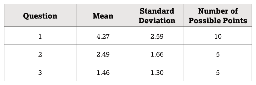
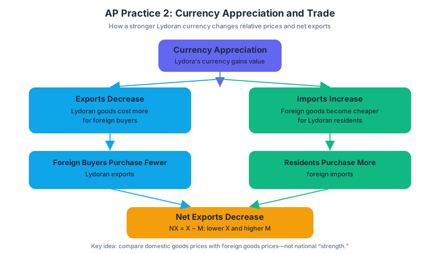
AP Practice 3
A short free-response question can test several economic skills at once: a student may need to make an assertion, explain a causal chain, calculate a value, and draw a correctly labeled graph—all in a tightly limited response.
AP Practice 3
A short free-response question can test several economic skills at once: a student may need to make an assertion, explain a causal chain, calculate a value, and draw a correctly labeled graph—all in a tightly limited response.
This original, unofficial practice set models the short free-response question (FRQ) task type. It is designed around the exam’s required response behaviors: assertions, explanations, numerical analysis, and graph creation. The economic setting is new; the task structure is not copied from released College Board material.
The task: policy in a recession
Assume an economy is experiencing a recessionary gap. The marginal propensity to consume is $0.75$. The government is considering an increase in government purchases of $40$ billion.
(a) Identify the type of fiscal policy that would reduce the recessionary gap.
(b) Calculate the maximum possible change in real gross domestic product resulting from the $40$ billion increase in government purchases.
(c) On a correctly labeled aggregate demand–aggregate supply graph, show the short-run effect of this policy on the price level and real output.
(d) Explain why the actual change in real output may be smaller than the maximum possible change.
Suggested timing: Spend about $8$ minutes. Reserve roughly $1$ minute to read and plan, $5$ minutes to write the economic reasoning and calculation, and $2$ minutes to draw and inspect the graph.
Step 1: Identify the policy
The economy has a recessionary gap, so real output is below full-employment output. An increase in government purchases is expansionary fiscal policy because it directly increases aggregate demand.
Core assertion: To reduce a recessionary gap, the government should use expansionary fiscal policy, such as increasing government purchases or decreasing taxes.
This response earns the identification point because it names both the policy direction and the policy category. Merely writing “fiscal policy” is incomplete: contractionary fiscal policy would move the economy in the wrong direction.
Step 2: Calculate the spending multiplier
The government-purchases multiplier is
$$ \text{Government-purchases multiplier}=\frac{1}{1-\text{MPC}}. $$
Substitute the given marginal propensity to consume:
$$ \frac{1}{1-0.75}
\frac{1}{0.25}
$$
The maximum possible change in real GDP is therefore
$$ \Delta Y
\text{multiplier}\times\Delta G
4\times $40\text{ billion}
$160\text{ billion}. $$
Answer to (b): Real GDP could increase by a maximum of $$160$ billion.
The word maximum matters. The calculation assumes that each round of additional income creates the full expected consumption response, with no taxes, imports, interest-rate effects, or supply constraints reducing the eventual increase.
Step 3: Draw the AD–AS response
The graph must include a vertical axis labeled Price Level and a horizontal axis labeled Real Output. Draw an upward-sloping Short-Run Aggregate Supply (SRAS) curve, a downward-sloping Aggregate Demand (AD) curve, and an initial equilibrium. Then shift AD rightward from $AD_1$ to $AD_2$.
The new short-run equilibrium has both a higher price level and higher real output. Label the initial equilibrium $(P_1,Y_1)$ and the new equilibrium $(P_2,Y_2)$, with $P_2>P_1$ and $Y_2>Y_1$.
A rightward shift of AD is essential. Moving along the original AD curve would show a change in quantity demanded caused by a price-level change, not the effect of an independent increase in government purchases.
Step 4: Explain why the actual increase may be smaller
The maximum multiplier result assumes that the entire induced increase in consumption continues through every spending round. In reality, some additional income may be saved, taxed, or spent on imports rather than on domestically produced goods and services.
The expansion can also raise the interest rate. Higher interest rates may reduce private investment and interest-sensitive consumption, creating a crowding-out effect that partially offsets the increase in aggregate demand. Therefore, the actual increase in real GDP may be less than $$160$ billion.
Full causal chain: Higher government purchases $\rightarrow$ higher aggregate demand $\rightarrow$ higher real output and price level in the short run; higher income, taxes, saving, imports, or interest rates may weaken the final output increase.
What an examiner rewards
| Task | Strong response | Common incomplete response |
|---|---|---|
| Assertion | Identifies expansionary fiscal policy and connects it to the recessionary gap | Says only “use fiscal policy” |
| Numerical analysis | Uses $\frac{1}{1-\text{MPC}}$ and calculates $$160$ billion | Uses the tax multiplier or forgets to multiply by $$40$ billion |
| Graph creation | Correctly labels axes, shifts AD right, and shows both outcomes | Shifts SRAS or draws movement along AD |
| Explanation | Gives a causal reason the actual result is smaller, such as crowding out or imports | Repeats that the multiplier is “not exact” without explaining why |
Named misconception check
Misconception: “A recession requires contractionary policy because the economy is performing badly.” The direction of policy depends on the problem being corrected. A recessionary gap requires an increase in aggregate demand, while excessive inflationary pressure may call for contractionary policy.
Misconception: “The multiplier result is always the final change in GDP.” The multiplier gives the maximum possible change under simplified assumptions. Leakage into saving, taxes, and imports, along with crowding out, can reduce the actual result.
Error-review routine
After completing the question, classify each error as one of four types: principle, interpretation, manipulation, or graphing and visuals. Rewrite only the missed part, adding the missing causal link, algebraic step, graph label, or directional explanation.
For a second attempt, cover the numerical answer and ask: What policy closes a recessionary gap? Which multiplier applies? Which curve shifts? What happens to the price level and real output? If those four answers are immediate, the response has the structure an examiner can reward.

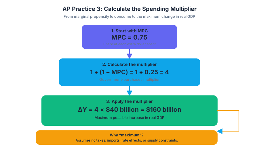
AP Practice 4
A strong short free-response answer does more than name a policy: it connects an economic model to a predicted outcome, supports the prediction with a graph or calculation, and explains the causal chain in precise language.
AP Practice 4
A strong short free-response answer does more than name a policy: it connects an economic model to a predicted outcome, supports the prediction with a graph or calculation, and explains the causal chain in precise language.
Task focus: short free-response analysis
This original, unofficial practice set models a short free-response task built around a change in monetary policy. It combines the four course skill categories: 1. Principles and Models, 2. Interpretation, 3. Manipulation, and 4. Graphing and Visuals.
Timing target: Spend approximately $12$–$15$ minutes. Reserve the final $2$ minutes to check graph labels, signs, units, and whether every “explain” prompt includes a cause-and-effect chain.
Practice prompt
Assume the economy is initially operating at full employment. The central bank decides to conduct an expansionary monetary policy.
(a) Draw a correctly labeled money market graph showing the effect of the policy on the equilibrium nominal interest rate. Identify the policy action that shifts the relevant curve.
(b) Explain how the change in the nominal interest rate affects investment spending, assuming other factors remain constant.
(c) Suppose the marginal propensity to consume is $0.75$. The central bank’s action increases planned investment by $$40$ billion. Calculate the maximum possible change in real gross domestic product generated by the investment increase.
(d) Using an aggregate demand–aggregate supply graph, show the short-run effect of the policy on real output and the price level. Assume the economy begins at full employment.
Worked reasoning
(a) Money market
Expansionary monetary policy increases the money supply. In the money market, the nominal interest rate is the price of borrowing money, so the vertical axis shows the nominal interest rate, $i$, and the horizontal axis shows the quantity of money, $M$.
The money-supply curve shifts right from $MS_1$ to $MS_2$. With money demand unchanged, the new equilibrium occurs at a lower nominal interest rate, moving from $i_1$ to $i_2$.
Credit-worthy graph response: The graph must label the vertical axis as the nominal interest rate, the horizontal axis as the quantity of money, show a downward-sloping money-demand curve, show the money-supply shift to the right, and indicate that the equilibrium interest rate decreases.
(b) Investment spending
A lower nominal interest rate reduces the cost of borrowing. Firms therefore face a lower financing cost for factories, equipment, inventories, or other capital projects, so planned investment spending increases.
The complete causal chain is:
$$ \text{Expansionary monetary policy} \rightarrow \text{money supply increases} \rightarrow i \text{ decreases} \rightarrow \text{borrowing becomes cheaper} \rightarrow I \text{ increases} $$
A response that merely says “investment increases because interest rates fall” identifies the correct relationship but may be incomplete if the prompt requires an explanation. Adding why lower interest rates encourage investment supplies the missing economic reasoning.
(c) Investment multiplier
The expenditure multiplier is calculated as:
$$\text{Multiplier}=\frac{1}{1-\text{MPC}}$$
Substitute the given marginal propensity to consume:
$$\text{Multiplier}=\frac{1}{1-0.75}=\frac{1}{0.25}=4$$
The maximum possible change in real GDP is:
$$\Delta Y=\text{Multiplier}\times\Delta I$$
$$\Delta Y=4\times $40\text{ billion}=$160\text{ billion}$$
Answer: Real GDP can increase by a maximum of $$160$ billion. The word maximum matters: this calculation assumes no crowding out, no taxes, no imports, and sufficient unused productive capacity.
(d) AD–AS effect
Higher investment spending is a component of aggregate demand:
$$AD=C+I+G+NX$$
Because investment, $I$, increases, aggregate demand shifts right from $AD_1$ to $AD_2$. In the short run, the economy moves upward along the unchanged short-run aggregate supply curve. Real output rises above its initial level, and the price level also rises.
The correct graph labels the vertical axis as the price level and the horizontal axis as real output, includes downward-sloping $AD$ and upward-sloping $SRAS$ curves, and shows $AD$ shifting right. The new equilibrium must have both a higher price level and greater real output.
Common misconceptions
Misconception 1: “Expansionary policy shifts money demand right.” The policy directly changes the money supply. Money demand may change later because income or the price level changes, but that is not the initial policy shift.
Misconception 2: “A lower interest rate reduces investment.” In the standard macroeconomic model, lower borrowing costs increase the quantity of investment demanded, holding expected profitability and other determinants constant.
Misconception 3: “The multiplier is $1-\text{MPC}$.” The multiplier is the reciprocal, $\frac{1}{1-\text{MPC}}$. With an MPC of $0.75$, each initial dollar ultimately creates up to $$4$ of total output.
Misconception 4: “Full employment means output cannot rise.” In the short run, expansionary policy can push real output above full-employment output, creating an inflationary gap. The economy may later self-adjust toward its long-run level.
What an examiner rewards
A rubric-aligned answer earns credit by showing the correct model, shifting the correct curve, calculating with the correct formula, and explaining the economic mechanism rather than stating disconnected conclusions. Numerical answers should include the calculation, not only the final number.
For error review, classify each missed point as model selection, curve shift, direction of change, calculation, graph labeling, or explanation. Then rewrite only the failed step, including the missing causal link or label; this is more useful than copying the entire answer.

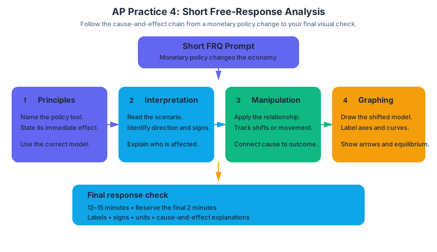
AP Practice 5
A short free-response question can test several macroeconomic skills at once: identifying a model, explaining a causal chain, calculating a numerical outcome, and interpreting the result in context.
AP Practice 5
A short free-response question can test several macroeconomic skills at once: identifying a model, explaining a causal chain, calculating a numerical outcome, and interpreting the result in context. The strongest responses do not merely state that a variable “increases” or “decreases”; they connect the change to a named economic mechanism.
Task type: Original, unofficial short free-response practice focused on assertions, explanations, numerical analysis, and graph creation.
Suggested timing: $15$ minutes, followed by $10$ minutes of error review.
Useful skill categories: 1. Principles and Models, 2. Interpretation, 3. Manipulation, and 4. Graphing and Visuals.
The scenario: a demand shock and stabilization policy
Suppose the economy of Lydora is experiencing a recessionary gap. Households become pessimistic about future income and reduce consumption spending by $20$ billion. The marginal propensity to consume is $0.75$. The price level is initially stable, and the government does not immediately change its fiscal policy.
The central question is: How large is the initial output effect, and what fiscal action could return real GDP to its potential level?
Practice prompt
(a) Draw a correctly labeled aggregate demand–aggregate supply graph showing the economy’s initial recessionary gap. Label the initial equilibrium price level $P_1$, real GDP $Y_1$, and potential output $Y_F$.
(b) Calculate the maximum possible change in real GDP resulting from the $20$ billion decrease in consumption spending. Show your work.
(c) Assume the government wants to offset the entire decrease in real GDP using only government purchases. Calculate the required change in government purchases.
(d) Explain why the actual change in real GDP may be smaller than the maximum possible change calculated in part (b).
(e) Instead of changing government purchases, suppose the government reduces lump-sum taxes. Explain why the required tax reduction would be larger than the required increase in government purchases.
Worked reasoning
(a) Constructing the AD–AS graph
Because reduced household consumption lowers aggregate demand, the economy moves leftward along the existing short-run aggregate supply curve from potential output to a lower level of real GDP. The graph must show a downward-sloping aggregate demand curve, an upward-sloping short-run aggregate supply curve, and a vertical long-run aggregate supply curve at $Y_F$.
A complete graph labels both axes: the vertical axis is the price level, and the horizontal axis is real GDP. The initial equilibrium occurs where $AD_1$ intersects $SRAS_1$, producing $P_1$ and $Y_1$, with $Y_1 < Y_F$.
(b) Applying the spending multiplier
The expenditure multiplier measures the total change in equilibrium real GDP generated by an initial change in autonomous spending:
$$ \text{Spending multiplier}=\frac{1}{1-\text{MPC}} $$
With a marginal propensity to consume of $0.75$:
$$ \text{Spending multiplier}=\frac{1}{1-0.75}=\frac{1}{0.25}=4 $$
The initial consumption decrease is $-\$20$ billion, so:
$$ \Delta Y=(4)(-$20\text{ billion})=-$80\text{ billion} $$
Answer: The maximum possible decrease in real GDP is $80$ billion.
(c) Selecting government purchases
A change in government purchases enters aggregate demand directly, so it receives the full spending multiplier. To offset the $80$ billion decrease in real GDP:
$$ \Delta Y=(\text{spending multiplier})(\Delta G) $$
$$ $80\text{ billion}=(4)(\Delta G) $$
$$ \Delta G=$20\text{ billion} $$
Answer: Government purchases must increase by $20$ billion, assuming the economy is in the multiplier model’s maximum-impact conditions.
(d) Why the maximum effect may not occur
The calculated $80$ billion effect assumes that each round of new income generates consumption according to the stated MPC, with no leakages beyond saving. In reality, households may save more, pay taxes, or purchase imported goods. These leakages reduce later rounds of spending, so the actual multiplier and output change may be smaller.
(e) Comparing purchases and taxes
A tax cut does not increase aggregate demand dollar for dollar because households initially spend only the fraction represented by the MPC. The tax multiplier is:
$$ \text{Tax multiplier}=-\frac{\text{MPC}}{1-\text{MPC}} $$
Here:
$$ \text{Tax multiplier}=-\frac{0.75}{0.25}=-3 $$
To raise real GDP by $80$ billion:
$$ $80\text{ billion}=(-3)(\Delta T) $$
$$ \Delta T=-$26.67\text{ billion} $$
Answer: Taxes must decrease by approximately $26.67$ billion. The reduction is larger than the $20$ billion increase in government purchases because only $75$ cents of each tax-cut dollar initially becomes consumption.
What earns credit
| Part | Examiner-rewarded reasoning |
|---|---|
| (a) | Correctly labeled axes, curves, equilibrium, and recessionary gap |
| (b) | Correct multiplier formula, substitution, and negative $80$ billion result |
| (c) | Uses the spending multiplier and identifies an increase in government purchases |
| (d) | Explains leakages or why the maximum multiplier may not be realized |
| (e) | Uses the tax multiplier and explains the MPC distinction |
Misconception check
Named misconception: “A $20$ billion spending decrease causes only a $20$ billion GDP decrease.” The initial decline is $20$ billion, but one person’s reduced spending becomes another person’s reduced income. Repeated rounds of lower consumption create the larger multiplied effect.
Retrieval check: If the MPC fell from $0.75$ to $0.50$, would the spending multiplier become larger or smaller? The answer is smaller: it would fall from $4$ to $2$, because each round of income produces less additional consumption.
Error-review routine
After completing the question, classify every error as one of four types: model error—the wrong graph or economic model; direction error—the correct model but the wrong increase/decrease; calculation error—incorrect formula or arithmetic; or communication error—an unsupported assertion, missing label, or absent unit. Redo only the missed part, then write one sentence explaining the causal chain: consumption falls → aggregate demand falls → equilibrium real GDP falls → multiplier rounds amplify the initial change.
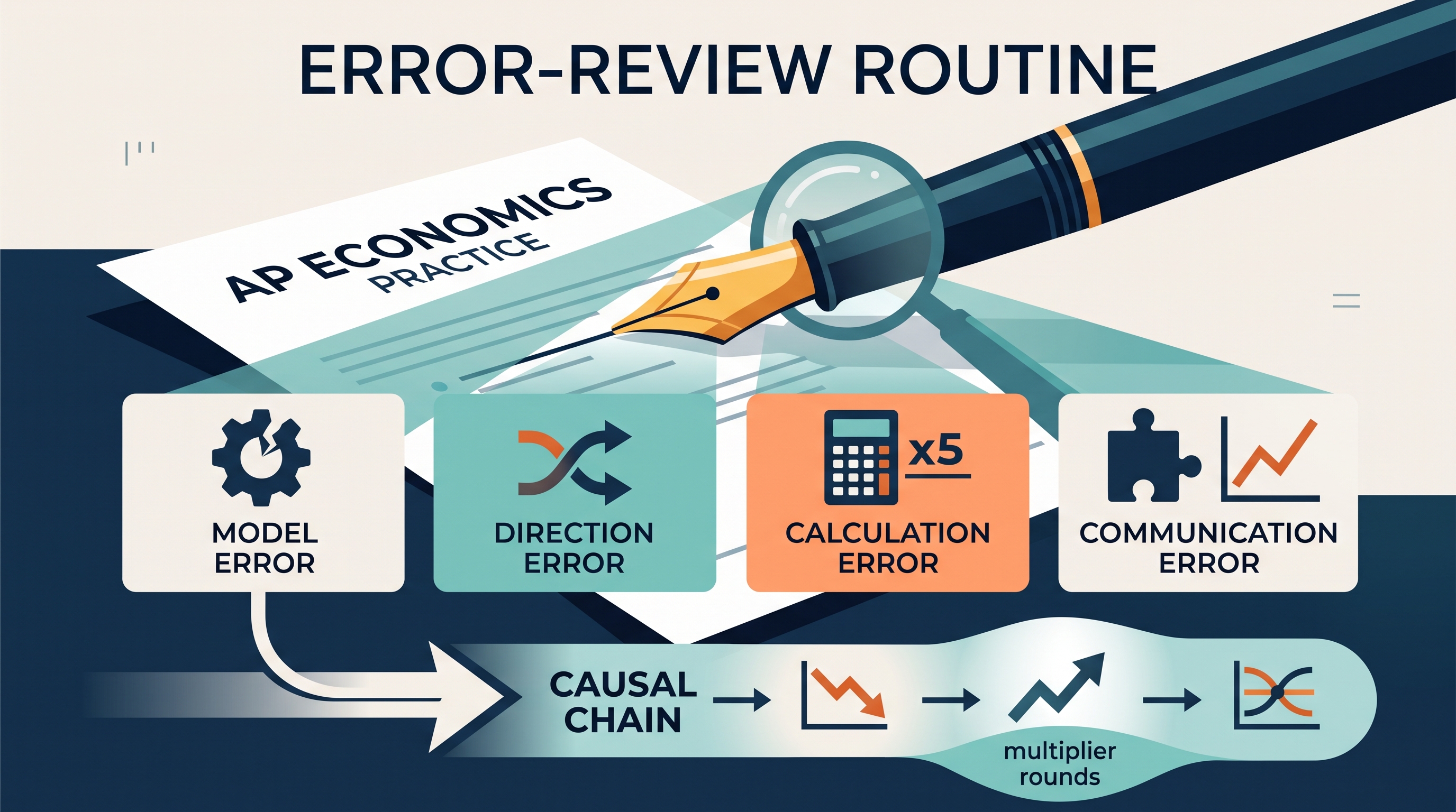
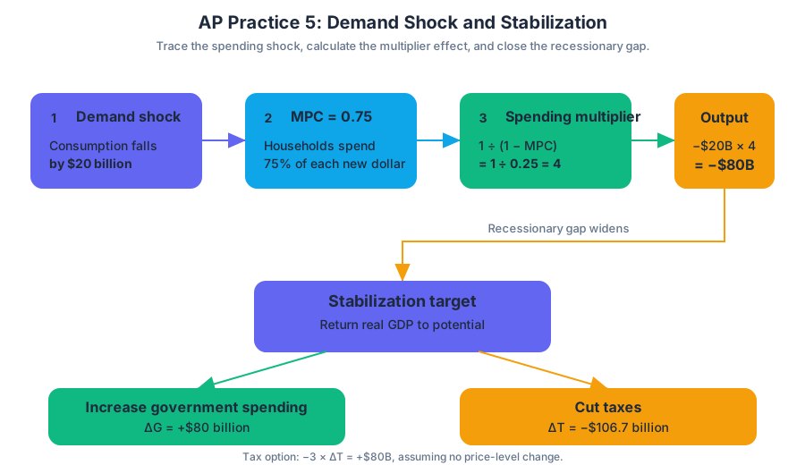
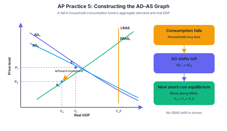
AP Practice 6
A rise in a country’s real interest rate can attract foreign investment, increase demand for its currency, and change its net exports. That chain links international capital flows, the foreign exchange market, and the balance of payments—exactly the kind of connected reasoning tested by a short free-response question.
AP Practice 6
A rise in a country’s real interest rate can attract foreign investment, increase demand for its currency, and change its net exports. That chain links international capital flows, the foreign exchange market, and the balance of payments—exactly the kind of connected reasoning tested by a short free-response question.
Task type: Short Free-Response Question
This original, unofficial practice task is designed as a short free-response question. On the current hybrid AP Macroeconomics Exam, students view the question in Bluebook and handwrite the response in a paper booklet. A practical target is about $15$ minutes: roughly $2$ minutes to identify the model, $8$ minutes to write and graph, and $5$ minutes to check causal direction and labels.
Exam habit: Every explanation should have a chain: economic change $\rightarrow$ market response $\rightarrow$ macroeconomic consequence.
Original practice prompt
The economy of Norland is initially at equilibrium. The domestic real interest rate rises relative to real interest rates in other countries.
(a) Identify the effect of the higher domestic real interest rate on the demand for Norland’s currency in the foreign exchange market. Explain.
(b) On a correctly labeled graph of the foreign exchange market for Norland’s currency, show the effect of the change in part (a). Label the initial equilibrium exchange rate $E_1$ and the new equilibrium exchange rate $E_2$.
(c) Indicate whether Norland’s currency appreciates or depreciates. Explain how the change affects Norland’s exports and imports.
(d) Indicate the effect on Norland’s net exports. Explain.
(e) Suppose the exchange rate changes from $1.20$ Norlandian currency units per euro to $1.32$ Norlandian currency units per euro. Calculate the percentage change in the value of the euro measured in Norlandian currency units.
Worked reasoning
(a) Currency demand
The demand for Norland’s currency increases. Foreign investors want to purchase Norlandian financial assets because those assets now offer a relatively higher real return. To buy those assets, investors must first acquire Norland’s currency.
This response earns the reasoning point because it identifies both the market change and its cause:
$$ \text{higher domestic real interest rate} \rightarrow \text{more foreign capital inflows} \rightarrow \text{greater demand for Norland’s currency} $$
(b) Foreign exchange graph
Draw the market for Norland’s currency with:
- vertical axis: exchange rate, measured as euros per Norlandian currency unit;
- horizontal axis: quantity of Norland’s currency;
- downward-sloping demand curve for Norland’s currency;
- upward-sloping supply curve for Norland’s currency;
- the demand curve shifting right from $D_1$ to $D_2$.
The equilibrium exchange rate rises from $E_1$ to $E_2$.
A graph must show the direction of the shift, not merely the final result. A rightward shift of demand creates excess demand at the original exchange rate, pushing the currency’s value upward until the new equilibrium is reached.
Graph-reading checkpoint
If the vertical axis instead measures Norlandian currency units per euro, the numerical direction of the exchange-rate movement would look different. Always read the axis before deciding whether the currency appreciates. Appreciation means the currency buys more foreign currency; it does not depend on which currency appears in the numerator of the quotation.
(c) Appreciation, exports, and imports
Norland’s currency appreciates because its value rises in the foreign exchange market. Norlandian goods become more expensive to foreign buyers, so Norland’s exports decrease. Foreign goods become less expensive to Norlandian buyers, so Norland’s imports increase.
$$ \text{currency appreciation} \rightarrow X \downarrow,\ M \uparrow $$
(d) Net exports
Norland’s net exports decrease because:
$$NX = X - M$$
Exports fall while imports rise, so:
$$NX \downarrow$$
The decrease in net exports also reduces aggregate demand because net exports are one component of planned expenditure:
$$AD = C + I + G + NX$$
(e) Percentage calculation
The value of the euro in Norlandian currency units increases from $1.20$ to $1.32$. Calculate the percentage change using:
$$\text{Percentage change}=\frac{\text{new value}-\text{old value}}{\text{old value}}\times 100$$
Substitute:
$$\frac{1.32-1.20}{1.20}\times 100 =\frac{0.12}{1.20}\times 100 =10%$$
The euro appreciates by $10%$ relative to the Norlandian currency. Equivalently, the Norlandian currency depreciates relative to the euro. The quotation is crucial: more Norlandian currency units are now needed to purchase one euro.
What the examiner rewards
| Response feature | Skill connection | What earns credit |
|---|---|---|
| Defines the capital-flow mechanism | Skill 1. Principles and Models | Uses the relationship between real interest rates and international investment |
| Explains the currency-demand shift | Skill 2. Interpretation | Connects higher returns to increased foreign demand for the currency |
| Calculates the percentage change | Skill 3. Manipulation | Shows the correct formula, substitution, and result |
| Draws and labels the graph | Skill 4. Graphing and Visuals | Labels axes, curves, shift direction, and both equilibria |
Named misconception check
Misconception: “A higher interest rate causes the currency supply to increase.” The immediate foreign-exchange effect emphasized here is an increase in demand for the domestic currency because foreigners are purchasing domestic assets. A student may discuss currency supplied by domestic investors purchasing foreign assets only if the situation specifically establishes increased purchases of foreign assets.
Error-review routine: After checking the answer, circle the first incorrect link in your chain. Was it the interest-rate effect, the currency-demand shift, the appreciation, the export-import relationship, or the calculation? Rewrite only that link in a complete sentence, then redraw the graph from memory.
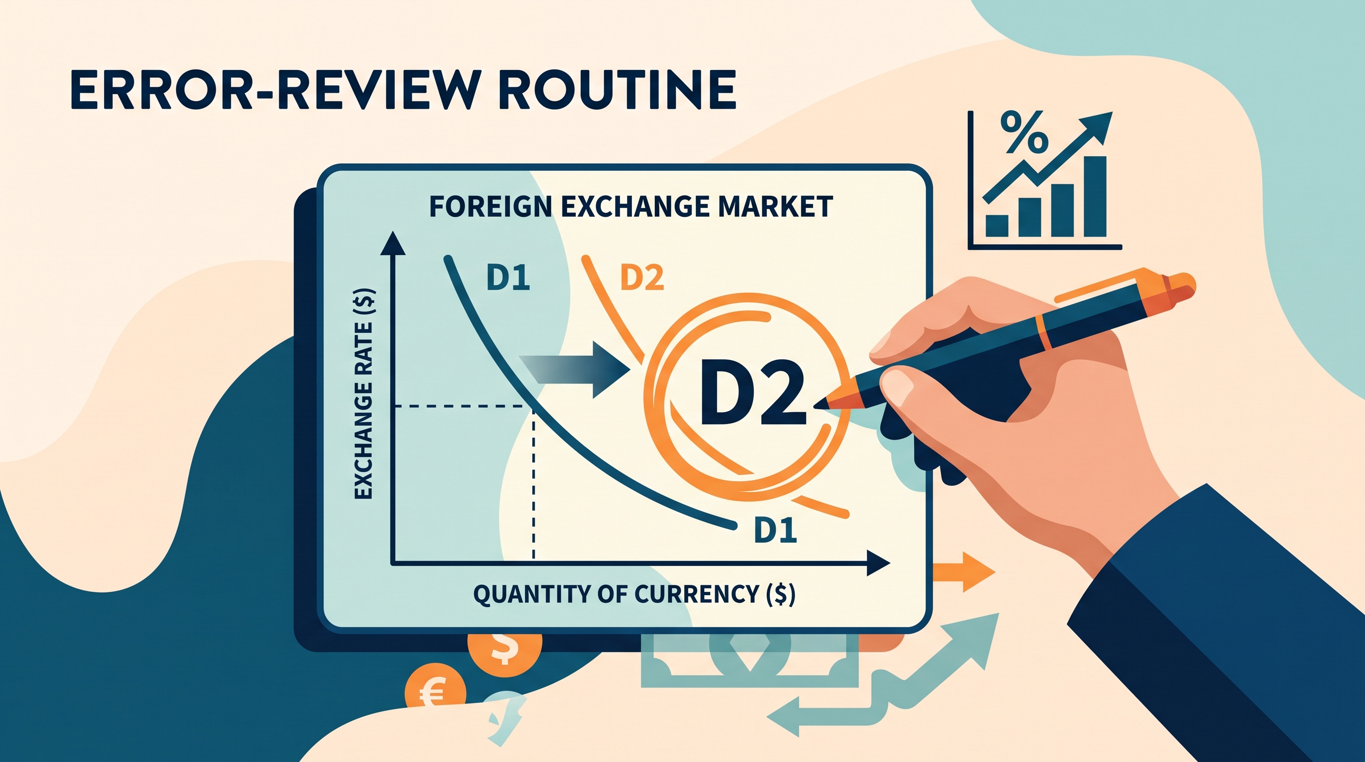
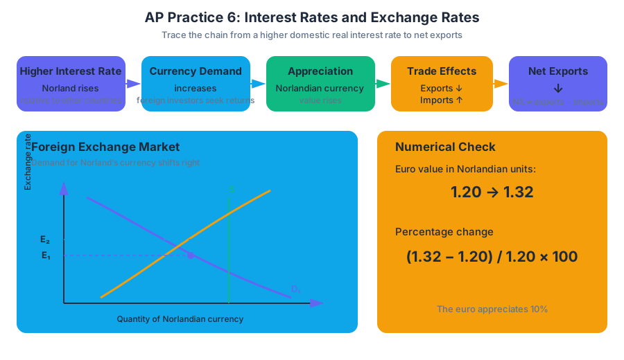
Source Materials
- AP Macroeconomics Course and Exam Description
- AP Macroeconomics Course and Exam Description Clarifications and Corrections
- AP Macroeconomics Course Overview
- AP Macroeconomics Course at a Glance
- AP Macroeconomics Course at a Glance Poster
- AP Macroeconomics
- AP Macroeconomics
- AP Macroeconomics Sample Syllabus 1
- Figure — AP Macroeconomics Course and Exam Description (p. 1)
- Figure — AP Macroeconomics Course and Exam Description (p. 17)
- Figure — AP Macroeconomics Course and Exam Description (p. 25)
- Figure — AP Macroeconomics Course and Exam Description (p. 26)
Study AP Macroeconomics with AI — Free on Lykke
Sign up for free to generate personalized flashcards, quizzes, and study guides from this course. Chat with an AI tutor that knows the material.
Get Started FreeView this course wiki on Lykke · Browse all public course wikis