AP Chemistry
Institution: MIT
95 study materials · 56 sections
AP Chemistry students working the current College Board Course and Exam Description, including first-time students with no prior background, plus teachers reviewing the page for CED alignment.; Teach every official CED unit and every numbered topic at topic granularity.; Develop every AP skill / science-practice code explicitly and by name.; Replace description with teaching: worked contextual examples, named misconceptions, and in-flow retrieval checks.; Build an exam-practice unit covering every task type on the current exam.
Course Sections
Course Framework, Skills and Reasoning Processes
Key concepts: Purpose of AP Chemistry as a college-level general chemistry course · Development of robust conceptual understanding applicable to future coursework and phenomena · Viewing chemical phenomena through macroscopic, microscopic, and symbolic levels · Using chemical models to analyze, explain, and predict phenomena · Supporting claims and conclusions with evidence · School-created curricula aligned with AP Chemistry content and skills · AP Course Audit requirements for schools offering AP courses · Organization of course content into commonly taught units · Science practices including questioning, data representation, and argumentation · Atomic structure as the foundation of the course
AP Chemistry asks a deceptively large question: How can observations of matter become explanations and predictions about invisible particles, energy, and change? A solution may fizz, a metal may conduct, or a spectrum may show separate lines; chemistry connects each visible event to a microscopic model and a…
Course Framework, Skills and Reasoning Processes
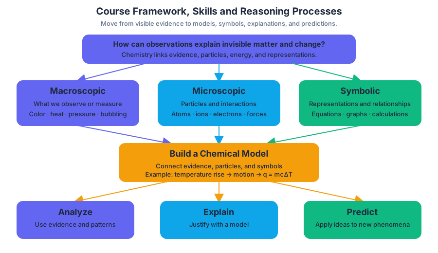
AP Chemistry asks a deceptively large question: How can observations of matter become explanations and predictions about invisible particles, energy, and change? A solution may fizz, a metal may conduct, or a spectrum may show separate lines; chemistry connects each visible event to a microscopic model and a symbolic representation such as an equation, graph, or calculation.
Core purpose: AP Chemistry is a challenging, research-based, college-level general chemistry course designed to develop a robust conceptual understanding of chemical principles that can be applied to future coursework and to unfamiliar phenomena.
That purpose is broader than memorizing reactions. Students learn to move among three levels of description:
- Macroscopic: what can be observed or measured, such as color, temperature, pressure, mass, or bubbling.
- Microscopic or sub-microscopic: particles and interactions, such as atoms, ions, molecules, electrons, and intermolecular forces.
- Symbolic: chemical formulas, balanced equations, graphs, mathematical relationships, and diagrams.
A strong explanation connects all three. For example, a temperature increase is a macroscopic observation; faster-moving particles provide a microscopic explanation; and $q = mc\Delta T$ supplies the symbolic relationship used to quantify the energy transfer. A chemical model is useful when it does more than illustrate an idea: it helps students analyze, explain, and predict phenomena.
The nine-unit content map
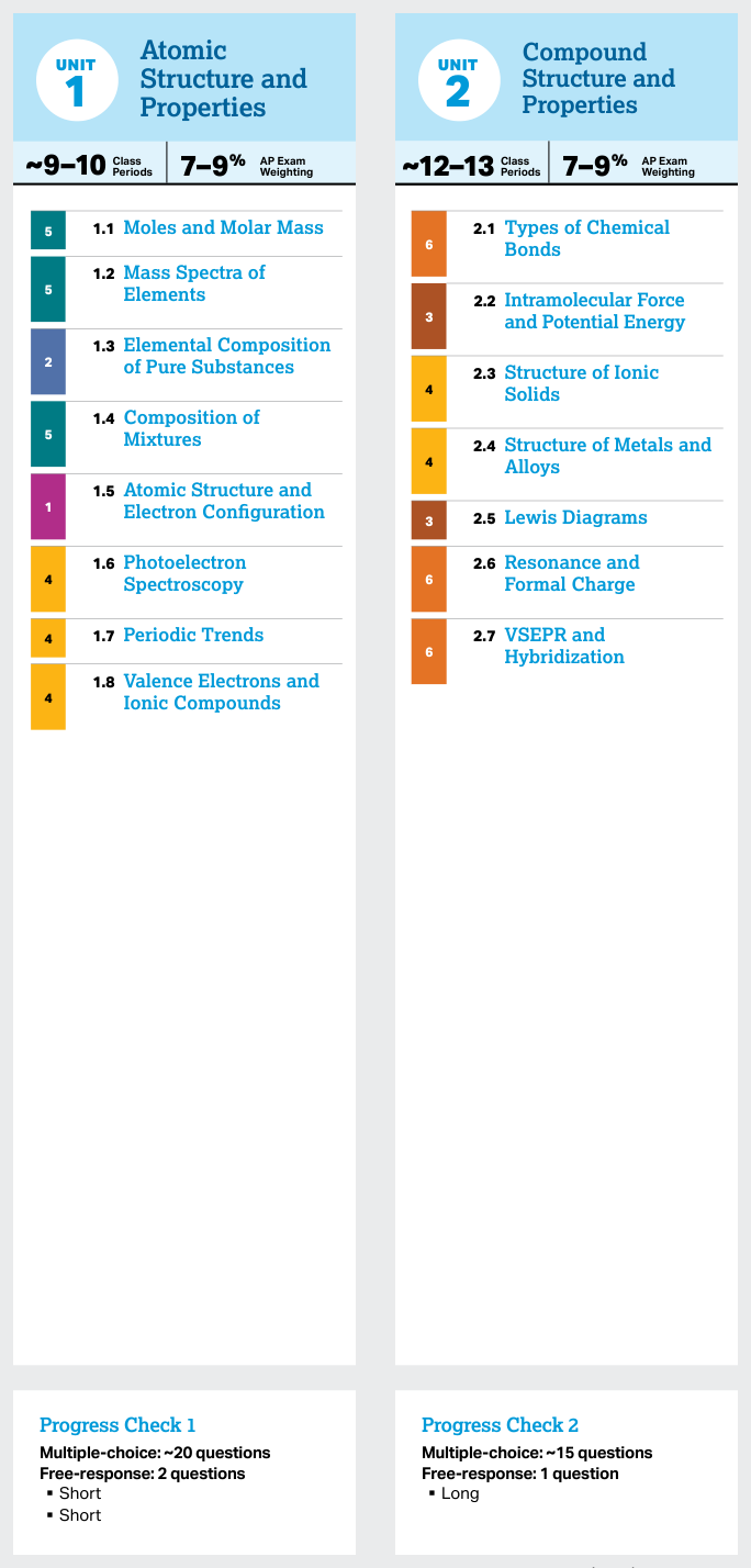
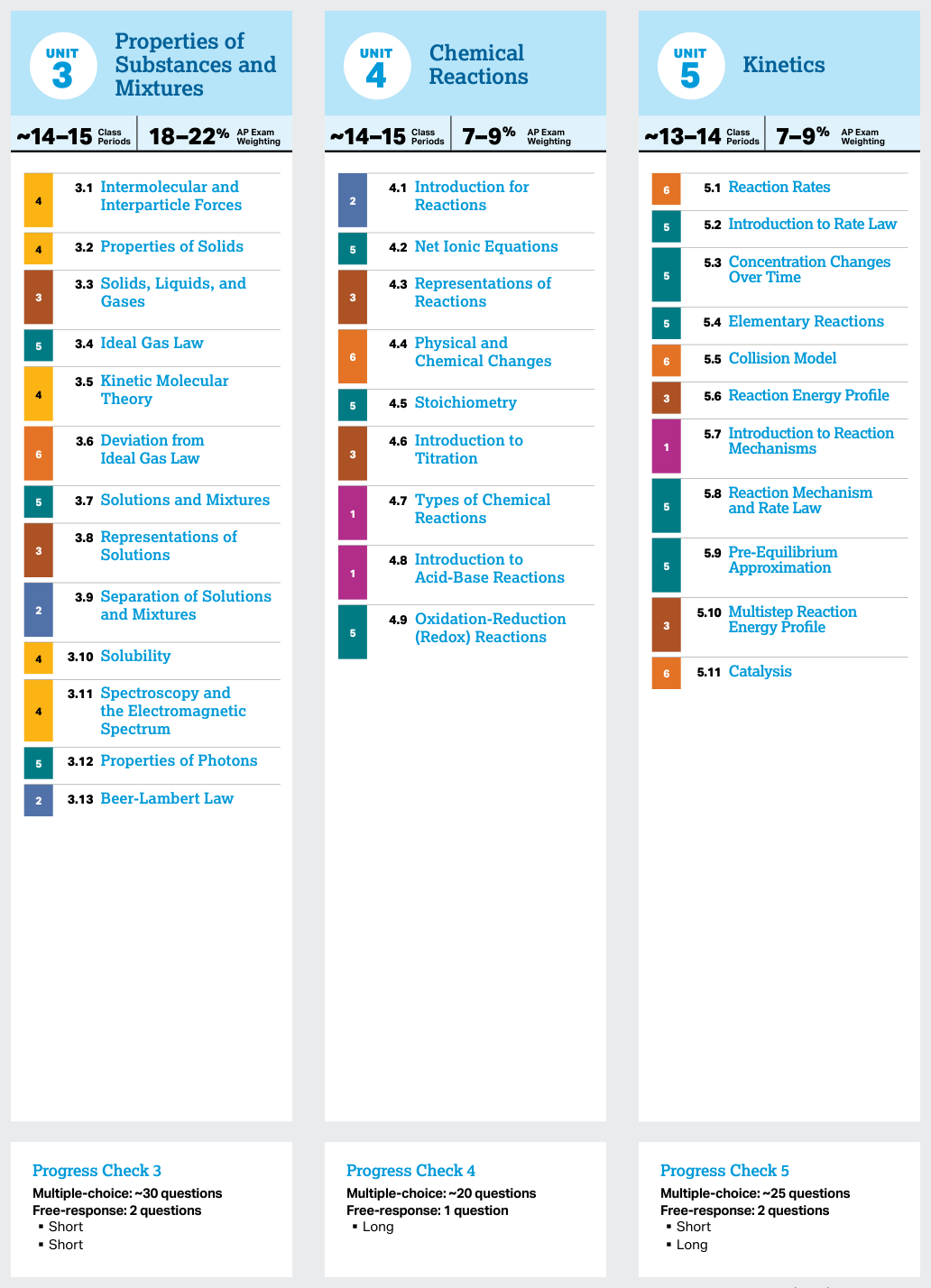
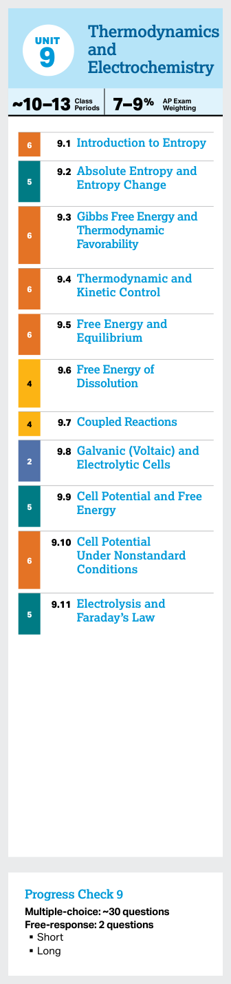
The framework organizes content into nine commonly taught units. Schools may adopt this sequence or modify it, but every required concept and skill must still be addressed. Unit 1, Atomic Structure and Properties, establishes the foundation: later explanations of bonding, reactions, spectra, periodic trends, and energy depend on a workable model of atoms and electrons.
| Unit | Multiple-choice exam weighting |
|---|---|
| Unit 1: Atomic Structure and Properties | $7%-9%$ |
| Unit 2: Compound Structure and Properties | $7%-9%$ |
| Unit 3: Properties of Substances and Mixtures | $18%-22%$ |
| Unit 4: Chemical Reactions | $7%-9%$ |
| Unit 5: Kinetics | $7%-9%$ |
| Unit 6: Thermochemistry | $7%-9%$ |
| Unit 7: Equilibrium | $7%-9%$ |
| Unit 8: Acids and Bases | $11%-15%$ |
| Unit 9: Thermodynamics and Electrochemistry | $7%-9%$ |
The weighting is guidance for emphasis, not a substitute for understanding. The science practices spiral through all nine units: a kinetics investigation may require a graph, a rate-law calculation, model analysis, experimental-error reasoning, and an evidence-based claim in the same task.
The six science practices
The practices describe what students do with chemistry knowledge. They are not isolated laboratory skills; they are reasoning tools used in multiple-choice questions, free-response questions, calculations, representations, and investigations.
Science Practice 1: Models and Representations requires students to describe chemical models and representations, including representations across scales, and to use them to communicate chemical structure, properties, and phenomena.
Science Practice 2: Question and Method requires students to determine scientific questions and methods. Its skills include identifying testable questions, proposing or describing experimental methods, collecting and analyzing data, attending to precision, identifying potential sources of experimental error (2.E), and explaining how a procedural modification will alter results (2.F).
Science Practice 3: Representing Data and Phenomena means creating representations or models of chemical phenomena:
- 3.A: Represent chemical phenomena using appropriate graphing techniques, including correct scale and units.
- 3.B: Represent chemical substances or phenomena with appropriate diagrams or models, such as an electron configuration.
- 3.C: Represent visually the relationship between structures and interactions across multiple levels or scales, such as particulate and macroscopic descriptions.
Science Practice 4: Model Analysis asks students to interpret models rather than merely draw them. Students describe what a model shows, identify relationships among its parts, use it to explain chemical behavior, recognize limitations, and determine whether a model supports a prediction or conclusion.
Science Practice 5: Mathematical Routines requires students to calculate an unknown quantity from known quantities by selecting and following a logical computational pathway. Dimensional analysis, appropriate units, precision, and significant figures are part of the reasoning—not cosmetic final steps.
Science Practice 6: Argumentation means developing an explanation or scientific argument:
- 6.A: Make a scientific claim.
- 6.B: Support a claim with evidence from experimental data.
- 6.C: Support a claim with evidence from representations or particulate-level models.
- 6.D: Provide reasoning using chemical principles, laws, or mathematical justification.
- 6.E: Connect particulate and macroscopic scales.
- 6.F: Connect experimental results with chemical concepts, processes, or theories.
- 6.G: Explain how experimental error may affect experimental results.
How the practices work together
A complete response follows a chain:
$$ \text{question} \rightarrow \text{method} \rightarrow \text{data} \rightarrow \text{representation} \rightarrow \text{model} \rightarrow \text{claim} $$
Suppose students investigate whether increasing temperature changes reaction rate. They identify a testable question (Science Practice 2: Question and Method), control relevant variables, measure time or concentration, graph the results (3.A), use collision-based reasoning (Science Practice 4: Model Analysis), calculate a rate (Science Practice 5: Mathematical Routines), and argue from evidence (Science Practice 6: Argumentation). If a thermometer responds slowly, 2.E, 2.F, and 6.G connect the error to the reliability of the conclusion.
Local curriculum, laboratories, and course authorization
The framework is not a complete day-by-day curriculum. Teachers create local curricula by selecting content and experiences that develop the required understandings and skills while meeting state or local requirements. Schools offering AP courses must participate in the AP Course Audit, demonstrate access to college-level resources, incorporate all required CED units and science practices, and connect chemistry to real-world questions.
Inquiry is central. At least $25%$ of instructional time is devoted to hands-on laboratory work, with a minimum of $16$ hands-on investigations, including at least $6$ guided-inquiry investigations; students maintain a laboratory notebook. A useful notebook records observations, data, calculations, representations, error analysis, and conclusions—evidence of the complete reasoning process rather than a polished answer alone.
Retrieval check
A sample is visibly blue, its particles are represented as ions in a diagram, and its concentration is calculated from absorbance. Identify the three levels of description, then name the practice used to justify a conclusion from the absorbance data. Answer: blue is macroscopic, the ion diagram is microscopic, concentration from absorbance is symbolic, and the evidence-based justification uses Science Practice 6: Argumentation, especially 6.B and 6.D.




1.1 Moles and Molar Mass · 1.2 Mass Spectra of Elements
Key concepts: Mole concept · Avogadro’s number · Molar mass · Converting between mass and amount of substance · Mass spectra of elements · Quantitative relationship between a mass spectrum and isotope masses · Quantitative relationship between a mass spectrum and isotope abundances · Learning objective 1.2.A · Mathematical routines (5.B) · Atomic Structure and Properties unit content
A mole is chemistry’s counting unit: just as a dozen means $12$ objects, one mole means $6.022\times10^{23}$ specified particles.
1.1 Moles and Molar Mass · 1.2 Mass Spectra of Elements
A mole is chemistry’s counting unit: just as a dozen means $12$ objects, one mole means $6.022\times10^{23}$ specified particles.
From particles to measurable samples
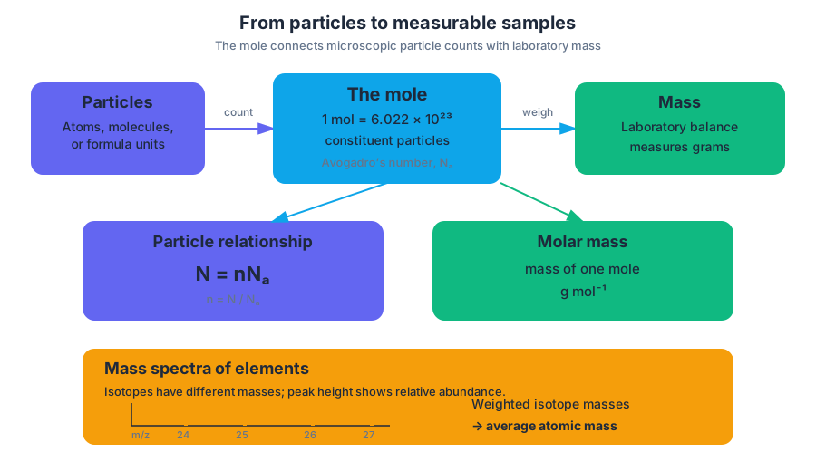
Atoms and molecules are far too small to count individually during a reaction, but laboratory balances measure mass. The mole connects those two scales: it tells us how many particles are present, while molar mass tells us what that amount weighs.
Avogadro’s number, $N_A=6.022\times10^{23}\ \mathrm{mol^{-1}}$, is the number of constituent particles in exactly one mole of a substance.
For an element, the particles may be atoms; for a molecular substance, they may be molecules; for an ionic compound, they are formula units. The numerical relationship is
$$ N=nN_A $$
where $N$ is the number of particles and $n$ is the amount of substance in moles. Conversely,
$$ n=\frac{N}{N_A} $$
A mole does not always mean the same mass: one mole of carbon atoms and one mole of iron atoms contain the same number of particles, but their atoms have different masses.
Molar mass: the mass of one mole
Molar mass is the mass of one mole of a substance, expressed in grams per mole, $\mathrm{g,mol^{-1}}$. Its numerical value comes from the substance’s atomic, molecular, or formula mass.
For example, the molar mass of calcium carbonate is found by adding the contributions of each atom:
$$ M(\mathrm{CaCO_3})
(1)(40.08)+(1)(12.01)+(3)(16.00)
100.09\ \mathrm{g,mol^{-1}} $$
The central conversion equation is
$$ n=\frac{m}{M} $$
where $n$ is amount in moles, $m$ is mass in grams, and $M$ is molar mass in $\mathrm{g,mol^{-1}}$.
Worked example: a mineral sample
A sample contains $25.0\ \mathrm{g}$ of $\mathrm{CaCO_3}$. How many moles of calcium carbonate does it contain?
$$ n=\frac{m}{M}
\frac{25.0\ \mathrm{g}}{100.09\ \mathrm{g,mol^{-1}}}
0.250\ \mathrm{mol} $$
The grams cancel, leaving moles. If the number of formula units is needed, continue:
$$ N=(0.250\ \mathrm{mol})(6.022\times10^{23}\ \mathrm{formula\ units,mol^{-1}}) $$
$$ N=1.51\times10^{23}\ \mathrm{formula\ units} $$
This is dimensional analysis in action: each conversion factor is chosen so unwanted units cancel.
Misconception check — “A mole is a mass.”
A mole measures amount of substance, not mass. The mass depends on particle identity. One mole of helium atoms has a much smaller mass than one mole of lead atoms, even though both samples contain $6.022\times10^{23}$ particles.
AP skill focus: Mathematical Routines
For 1.1 Moles and Molar Mass, the key mathematical routine is selecting an appropriate relationship and applying it with units. The relevant course-framework pairing is 1.B Identify an appropriate theory, definition, or mathematical relationship to solve a problem; the topic page also identifies Mathematical Routines (5.B) with the same mathematical emphasis.
A strong solution identifies the target quantity, writes the relationship before substituting values, carries units through every step, and reports a reasonable number of significant figures.
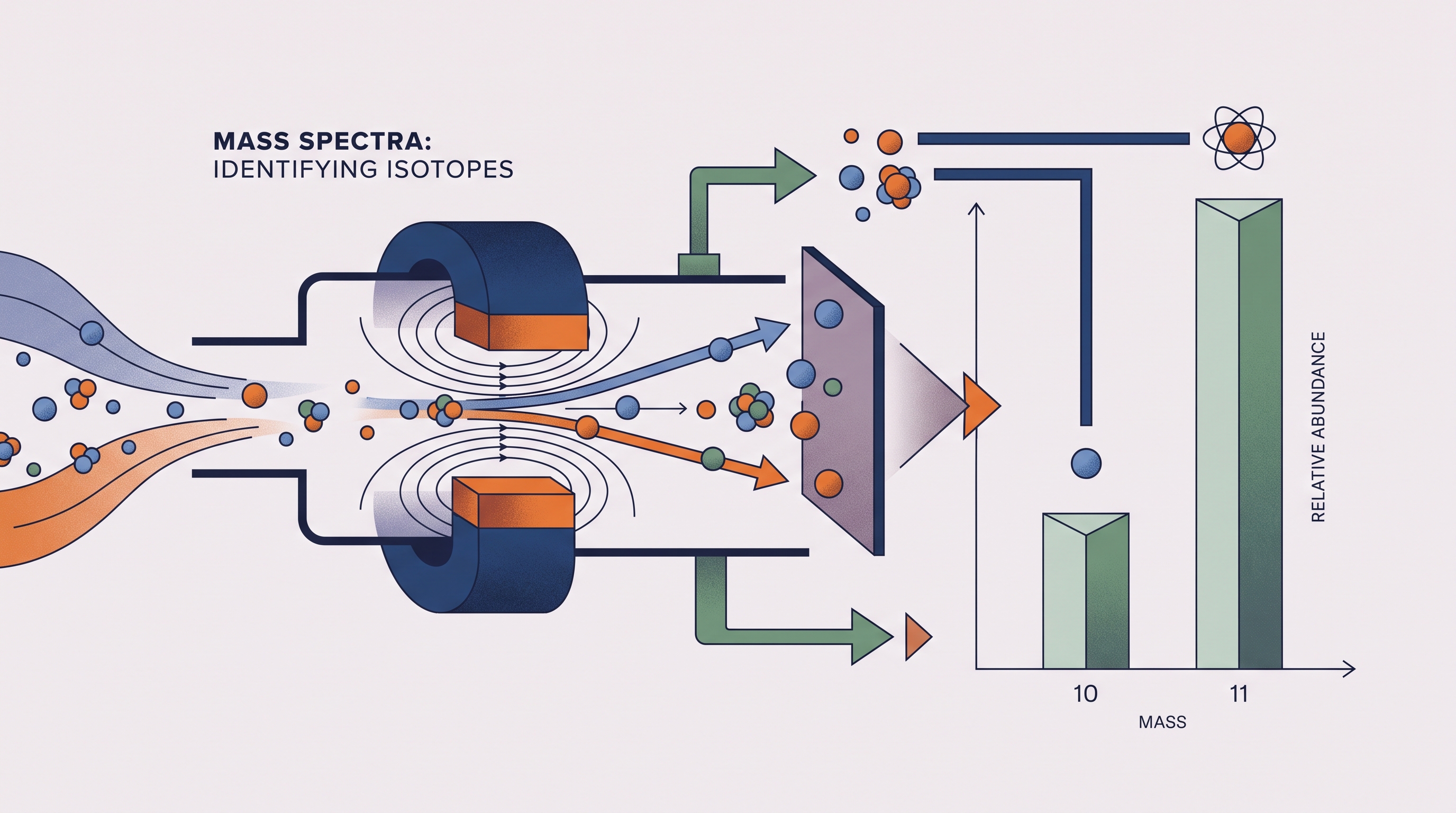
Mass spectra: counting isotopes by mass
A mass spectrum displays the particles detected from a sample according to their mass-to-charge ratio, commonly written as $m/z$. For singly charged positive ions, $z=1$, so the location of a peak is approximately the isotope’s mass.
Each peak corresponds to particles with a particular mass. The peak’s horizontal position identifies an isotope’s mass, while its relative height or intensity indicates the isotope’s relative abundance in the sample.
Learning Objective 1.2.A: Explain the quantitative relationship between the mass spectrum of an element and the masses of the element’s isotopes.
Essential Knowledge 1.2.A.1: The mass spectrum of a sample containing a single element can be used to determine the identity of the isotopes of that element and the relative abundance of each isotope in nature.
Worked interpretation: two isotope peaks
Imagine an element whose spectrum has two peaks:
| Peak position | Relative abundance |
|---|---|
| $35$ | $75%$ |
| $37$ | $25%$ |
The element contains two isotopes, one with mass approximately $35$ and one with mass approximately $37$. The taller peak means the mass-$35$ isotope is more abundant; it does not mean each individual atom is lighter because it is more abundant.
The abundance-weighted average mass is
$$ \overline{m}
(0.75)(35)+(0.25)(37)
35.5 $$
Thus, the periodic-table atomic mass would lie between the isotope masses and closer to $35$ because that isotope is more common.
AP skill focus: reading graphical evidence
For 1.2 Mass Spectra of Elements, the suggested skill is 1.C Identify information presented graphically to solve a problem. Read the spectrum in two directions: use the $m/z$ values to identify particle masses, then use peak intensities to compare relative abundances. Do not confuse a peak’s position with its height.
Retrieval check: A spectrum has peaks at $10$ and $11$, with the $11$ peak three times as tall as the $10$ peak. Which isotope is more abundant, and which feature of the graph supports your answer?
Answer: The mass-$11$ isotope is more abundant; the taller peak represents its greater relative abundance. The horizontal positions identify masses, while vertical intensity compares abundance.
1.3 Elemental Composition of Pure Substances · 1.4 Composition of Mixtures
Key concepts: Pure substances · Elemental composition by mass · Empirical formulas · Fixed mass ratios in compounds · Mixtures · Variable relative proportions in mixtures · Elemental analysis · Homogeneous solutions · Heterogeneous mixtures · Macroscopic properties of mixtures
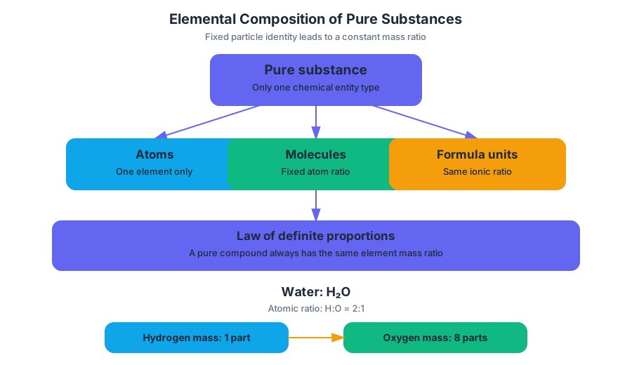
A pure compound has a chemical identity that does not change from sample to sample: the elements occur in a fixed ratio, so the mass ratio of those elements is constant.
1.3 Elemental Composition of Pure Substances · 1.4 Composition of Mixtures
A pure compound has a chemical identity that does not change from sample to sample: the elements occur in a fixed ratio, so the mass ratio of those elements is constant. A mixture is different—its components may be present in almost any relative proportions. This distinction lets chemists identify substances, determine purity, and calculate how much of a desired component is present.
Pure substances and fixed composition
A pure substance contains only one type of chemical entity: individual atoms, molecules, or formula units. A sample of pure water contains only $H_2O$ molecules; a sample of pure sodium chloride contains formula units with the same $Na:Cl$ ratio. The particles may be too small to see, but their composition is not arbitrary.
Law of definite proportions: In any pure sample of a particular compound, the ratio of the masses of its constituent elements is always the same.
For example, every pure sample of water has hydrogen and oxygen atoms in a $2:1$ ratio. Because oxygen atoms are much more massive than hydrogen atoms, the mass ratio is not $2:1$; it is approximately $1:8$. A small drop and a large lake differ in total mass, but not in the relative mass contributions of hydrogen and oxygen.
From mass composition to an empirical formula
The elemental composition by mass is the percentage of a compound’s total mass contributed by each element:
$$ % \text{ element}= \frac{\text{mass of element}}{\text{total mass of compound}}\times 100% $$
The empirical formula gives the lowest whole-number ratio of atoms in a compound. Elemental analysis connects the two: measured masses become moles, mole amounts become a ratio, and that ratio becomes the empirical formula. This uses the molar-mass conversions established earlier, but the goal here is different: determining the atom ratio that defines the substance.
Worked example: finding an empirical formula
A compound contains $40.0%$ carbon, $6.7%$ hydrogen, and $53.3%$ oxygen by mass. Assume a $100.0\text{-g}$ sample, so the percentages become convenient masses:
$$ 40.0\text{ g C},\qquad 6.7\text{ g H},\qquad 53.3\text{ g O} $$
Convert each mass to moles:
$$ n_C=\frac{40.0\text{ g}}{12.01\text{ g mol}^{-1}}=3.33\text{ mol} $$
$$ n_H=\frac{6.7\text{ g}}{1.008\text{ g mol}^{-1}}=6.65\text{ mol} $$
$$ n_O=\frac{53.3\text{ g}}{16.00\text{ g mol}^{-1}}=3.33\text{ mol} $$
Divide every mole amount by the smallest amount, $3.33\text{ mol}$:
$$ C:H:O=1.00:2.00:1.00 $$
Therefore, the empirical formula is
$$ \boxed{CH_2O} $$
The formula need not describe a molecule containing only three atoms. For an ionic substance, it represents the lowest ratio in a formula unit; for a molecular substance, the actual molecular formula may be a whole-number multiple of the empirical formula.
Misconception check: Percent composition does not directly give subscripts. A percentage describes mass, whereas a formula describes numbers of atoms. Always convert mass to moles before finding the ratio.
Mixtures: composition can vary
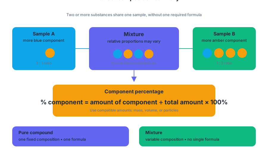
A mixture contains two or more types of atoms, molecules, or formula units whose relative proportions can vary. Salt water, soil, air, and a solid containing sodium bicarbonate mixed with another compound are mixtures. Unlike a pure compound, a mixture does not have one required chemical formula.
The composition of a mixture can be reported using amounts or percentages:
$$ % \text{ component}= \frac{\text{amount of component}}{\text{total amount of mixture}}\times100% $$
The “amount” might be mass, volume, number of particles, or another clearly specified quantity. The denominator and numerator must use compatible quantities.
Homogeneous and heterogeneous mixtures
In a solution, a homogeneous mixture, macroscopic properties do not vary throughout the sample. A thoroughly mixed salt solution has the same concentration and appearance in every location, even though the particles are distributed among solvent particles.
In a heterogeneous mixture, macroscopic properties depend on location. A scoop of soil may contain different amounts of sand, clay, organic matter, and water depending on where the scoop is taken. Sampling location therefore matters when estimating composition.
Misconception check: “Uniform-looking” and “pure” do not mean the same thing. A solution can be uniform throughout while still containing several substances.
Quantitative analysis: percentage of $NaHCO_3$
Suppose a $5.00\text{-g}$ mixture contains sodium bicarbonate, $NaHCO_3$, along with an inert solid. If quantitative analysis determines that the mixture contains $2.00\text{ g}$ of $NaHCO_3$, then
$$ %NaHCO_3= \frac{2.00\text{ g}}{5.00\text{ g}}\times100%=40.0% $$
This calculation describes the mixture’s composition, not the empirical formula of sodium bicarbonate. The formula $NaHCO_3$ describes a pure compound with fixed elemental proportions; $40.0%$ describes how much of that compound is present in a particular mixture.
AP skill in action
This topic develops Science Practice 5: Mathematical Routines, especially 5.A: Identify quantities needed to solve a problem from given information (e.g., text, mathematical expressions, graphs, or tables). In an empirical-formula problem, identify element masses or percentages, molar masses, and mole ratios. In a mixture problem, identify the component amount and the total mixture amount before selecting the percentage relationship.
Retrieval check
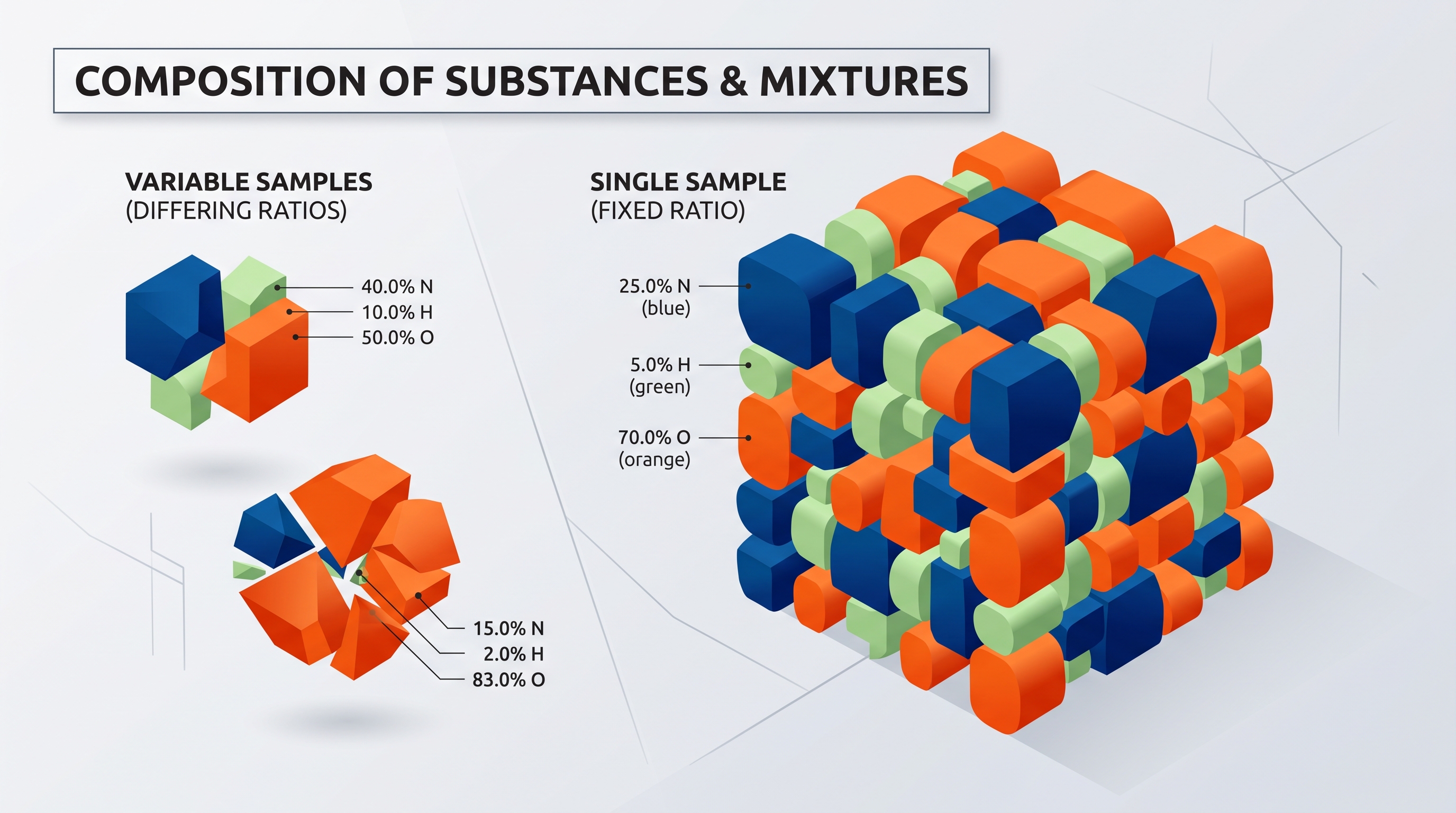
A sample is reported as $25.0%$ nitrogen, $5.0%$ hydrogen, and $70.0%$ oxygen by mass. Is it necessarily a mixture? No. Those data could describe a pure compound if the percentages correspond to a fixed empirical formula. By contrast, if two samples of the same material have different component percentages, the material is behaving as a mixture rather than as one pure compound.
1.5 Atomic Structure and Electron Configuration · 1.6 Photoelectron Spectroscopy
Key concepts: Atomic structure · Electron configuration · Periodic trends as a function of atomic number · Valence electrons · Quantum mechanics · Aufbau principle · Photoelectron spectroscopy (PES) · Interpreting graphical data · Models and representations of particulate-level properties · Connecting macroscopic and particulate scales
An atom’s chemical behavior depends strongly on how its electrons are distributed among allowed energy levels, and photoelectron spectroscopy (PES) provides experimental evidence for that distribution.
1.5 Atomic Structure and Electron Configuration · 1.6 Photoelectron Spectroscopy
An atom’s chemical behavior depends strongly on how its electrons are distributed among allowed energy levels, and photoelectron spectroscopy (PES) provides experimental evidence for that distribution.
From atomic number to electron configuration
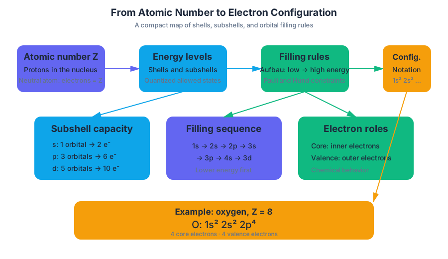
The atomic number, $Z$, gives the number of protons in an atom and, for a neutral atom, also the number of electrons. Because electrons occupy quantized energy states rather than arbitrary locations, an atom can be represented by an electron configuration: a notation showing how its electrons are distributed among shells and subshells.
Essential Knowledge 1.5.A.3: Electrons can be viewed as occupying “shells,” or energy levels, and “subshells,” or sublevels. Inner electrons are core electrons; outer electrons are valence electrons. The electron configuration is explained by quantum mechanics, the Aufbau principle, and the organization of the periodic table.
Quantum mechanics predicts the allowed electron states. The Aufbau principle provides the filling order: electrons occupy available orbitals from lower energy to higher energy. The Pauli exclusion principle limits each orbital to two electrons with opposite spins, while Hund’s rule places electrons singly into equal-energy orbitals before pairing them.
A compact filling sequence is:
$$ 1s,\ 2s,\ 2p,\ 3s,\ 3p,\ 4s,\ 3d,\ 4p,\ 5s,\ldots $$
The superscript gives the number of electrons in that subshell. For example, oxygen has $Z=8$ and therefore eight electrons:
$$ \mathrm{O}: 1s^2 2s^2 2p^4 $$
The first four electrons are core electrons, while the electrons in the outermost occupied shell, $n=2$, are valence electrons. Electron configurations therefore connect the particulate scale to measurable chemical behavior; one mole of oxygen atoms contains $6.022\times10^{23}$ copies of this electron arrangement.
Reading configurations as models
An electron configuration is a model—a symbolic representation of a particulate-level structure, not a literal photograph of electrons traveling along fixed circular paths. The periodic table reflects the periodicity of element properties as a function of atomic number because elements in related positions develop related outer-electron patterns.
For ions, adjust the electron count using the charge. A magnesium atom has twelve electrons:
$$ \mathrm{Mg}: 1s^2 2s^2 2p^6 3s^2 $$
A magnesium ion, $\mathrm{Mg^{2+}}$, has lost two electrons:
$$ \mathrm{Mg^{2+}}: 1s^2 2s^2 2p^6 $$
A common misconception is that the charge changes the number of protons. It does not: ion formation changes the number of electrons, while the proton count—and therefore the element’s identity—remains fixed.
Scope boundary: “The assignment of quantum numbers to electrons in subshells of an atom will not be assessed on the AP Exam.” The required reasoning is the use and interpretation of electron configurations, not the assignment of individual quantum-number sets.
Photoelectron spectroscopy: turning peaks into electrons
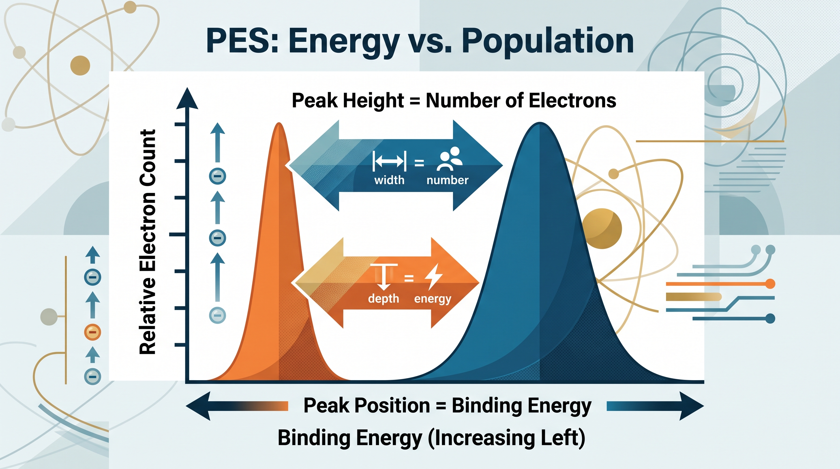
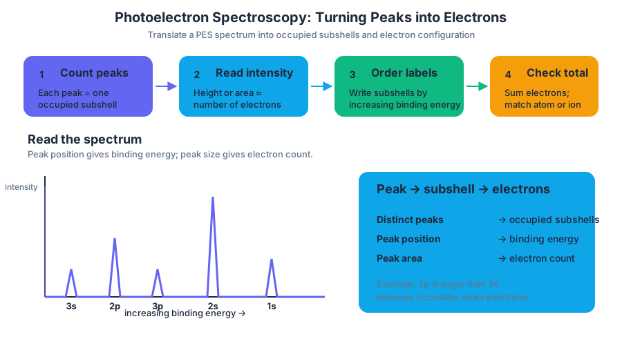
Photoelectron spectroscopy measures the energy required to remove electrons from an atom. Each peak corresponds to a subshell, and the peak’s position indicates the electron-binding energy. A peak representing more electrons is ideally taller or has greater area.
Essential Knowledge 1.6.A.1: The energy required to remove an electron from a subshell is related to the location of its peak in a PES spectrum, while the relative height of a peak is ideally proportional to the number of electrons in that subshell.
The interpretation is easiest when treated as a translation problem:
- Count the distinct peaks to identify occupied subshells.
- Read relative peak intensities to determine how many electrons occupy each subshell.
- Write the subshell labels in order of increasing binding energy.
- Check that the total electron count matches the element or ion.
Worked example: reconstructing an atom
Suppose a PES spectrum shows four subshell peaks with relative electron populations of $2$, $2$, $6$, and $1$. The total is:
$$ 2+2+6+1=11\ \text{electrons} $$
The configuration is therefore:
$$ 1s^2 2s^2 2p^6 3s^1 $$
An atom with eleven electrons is sodium, $\mathrm{Na}$. The single $3s$ electron is a valence electron, while the other ten are core electrons.
The reverse reasoning also works. Given $\mathrm{Al}$, with $Z=13$:
$$ \mathrm{Al}: 1s^2 2s^2 2p^6 3s^2 3p^1 $$
its PES spectrum should contain five occupied-subshell peaks, with relative populations $2:2:6:2:1$. The $1s$ electrons generally require the greatest energy to remove because they are closest to the nucleus and experience strong attraction.
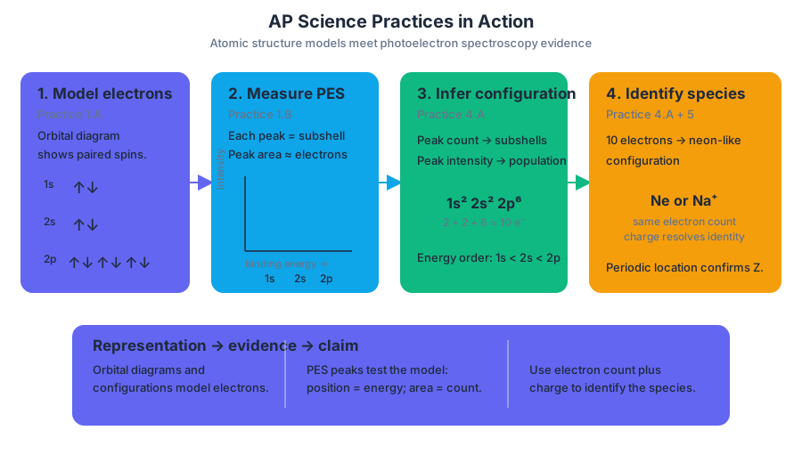
AP Science Practices in action
- Science Practice 1: Models and Representations — Skill 1.A, “Describe representations and models of natural phenomena.” Use orbital diagrams, electron configurations, and periodic-table locations to represent electron distributions.
- Science Practice 1: Models and Representations — Skill 1.B, “Explain models and representations.” Explain why a peak corresponds to a subshell and why peak intensity reflects electron population.
- Science Practice 4: Model Analysis — Skill 4.A, “Explain how models or representations describe chemical phenomena.” Infer an electron configuration from a PES graph, then use that configuration to identify the element or ion.
- Science Practice 5: Mathematical Routines — Skill 5.A, “Identify and describe the components of a scientific problem.” Track electron counts, ionic charge, peak populations, and mole-to-particle conversions without losing the scale being used.
Misconception check
A taller PES peak does not mean that the electrons in that subshell have higher energy. Peak position represents the energy required to remove electrons; peak height or area represents how many electrons are present. Ask yourself: Am I reading the horizontal axis for binding energy and the vertical dimension for population?
Retrieval check: A species has the configuration $1s^2 2s^2 2p^6 3s^2 3p^5$. How many core electrons, valence electrons, and total electrons does it contain? The answer is $10$ core electrons, $7$ valence electrons, and $17$ total electrons.
1.7 Periodic Trends · 1.8 Valence Electrons and Ionic Compounds
Key concepts: Periodic trends in atomic and molecular properties · Valence electrons and their relationship to an element’s location on the periodic table · Typical ionic charges of atoms · Formation and bonding in binary ionic compounds · Coulomb’s law as a basis for periodic trends · Shell model of atomic structure · Electron shielding and effective nuclear charge · Exceptions to expected periodic trends · Connecting particulate-level structure to macroscopic properties using models and representations
The periodic table is not merely an index of elements: its position predicts how strongly an atom holds electrons, how large it is, and what ions it tends to form.
1.7 Periodic Trends · 1.8 Valence Electrons and Ionic Compounds
The periodic table is not merely an index of elements: its position predicts how strongly an atom holds electrons, how large it is, and what ions it tends to form. The central question is: How can an element’s location predict both its microscopic bonding behavior and the macroscopic properties of its compounds?
The shell model behind periodicity
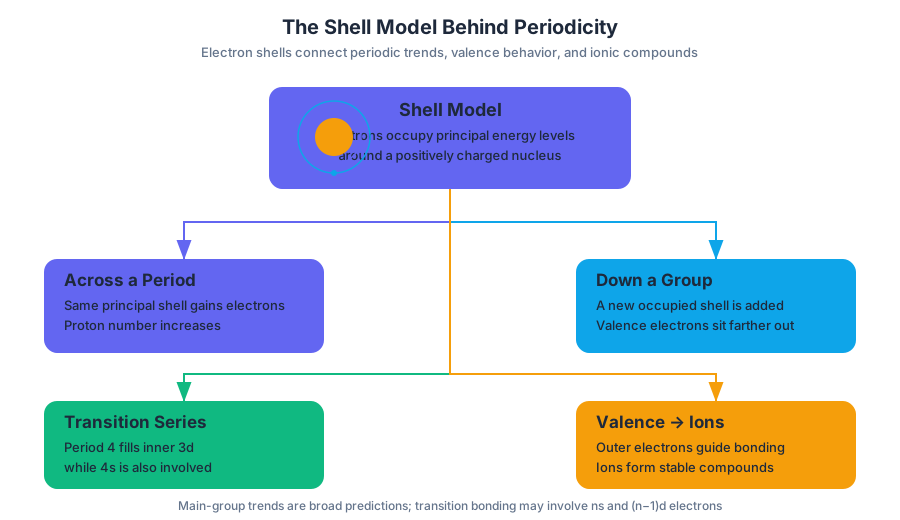
The shell model places electrons in principal energy levels, or shells, around the nucleus. For main-group elements, moving across a period generally adds electrons to the same principal shell while the number of protons increases. Moving down a group adds a new occupied shell, so the valence electrons are farther from the nucleus.
This simple picture requires an important qualification. In the transition series, electrons can enter an inner $(n-1)d$ subshell rather than the newest outer shell; for example, period-4 transition elements fill the $3d$ subshell while the $4s$ subshell is also involved. Therefore, the main-group shell model predicts broad trends especially well, while transition-element bonding may involve both $ns$ and incompletely filled $(n-1)d$ electrons.
Why periodic trends occur
Coulomb’s law states that the electrostatic attraction between opposite charges becomes stronger when charge magnitudes increase and weaker when distance increases:
$$F = k\frac{|q_1q_2|}{r^2}$$
Inner electrons partially block the nucleus from attracting outer electrons. This effect is called shielding. The net positive attraction experienced by an electron is the effective nuclear charge, often represented as $Z_{\text{eff}}$. Across a main-group period, nuclear charge increases while shielding changes less dramatically because electrons are added mainly to the same shell. Thus, $Z_{\text{eff}}$ generally increases.
Down a group, additional shells increase both distance and shielding. Even though the nucleus contains more protons, the outer electron is usually held less tightly because the $r^2$ effect and shielding outweigh the increased nuclear charge.
| Property | Across a period, left to right | Down a group | Why |
|---|---|---|---|
| Atomic radius | Generally decreases | Generally increases | Nuclear attraction versus shell distance |
| Ionization energy | Generally increases | Generally decreases | Energy required to remove an electron |
| Electronegativity | Generally increases | Generally decreases | Attraction for bonding electrons |
| Electron affinity | Generally becomes more favorable overall | Generally less favorable overall | Energy change when an electron is added |
| Ionic radius | Cations are smaller; anions are larger than their atoms | Generally increases | Electron loss or gain plus shell structure |
Ionization energy is the energy required to remove an electron from a gaseous atom. A smaller radius and larger $Z_{\text{eff}}$ make removal harder. Electronegativity describes how strongly an atom attracts shared electrons in a bond. Electron affinity describes the energy change when a gaseous atom gains an electron; its numerical sign convention must be read carefully because “more favorable” does not always mean “larger positive number.”
Periodic trends are predictions, not rigid laws. Small exceptions occur when subshell energies and electron pairing alter stability. For example, the first ionization energy of boron is slightly lower than that of beryllium because boron’s removed electron is in a higher-energy $2p$ subshell; oxygen’s is slightly lower than nitrogen’s because oxygen has paired electrons in a $2p$ orbital. The CED does not require writing electron configurations for exceptions to the aufbau principle, but it does require reasoning from models such as shielding and $Z_{\text{eff}}$.
Valence electrons and typical ionic charges
Valence electrons are electrons available for bonding. For main-group elements, these are usually the electrons in the outermost occupied shell. For transition elements, valence electrons can include electrons in an incompletely filled inner $(n-1)d$ subshell as well as $ns$ electrons.
Main-group atoms often form ions that achieve a more stable electron arrangement. Their typical charges follow their periodic-table columns:
| Group | Typical ion | Electron change |
|---|---|---|
| Group 1 | $+1$ | Loses one valence electron |
| Group 2 | $+2$ | Loses two |
| Group 13 | $+3$ | Often loses three |
| Group 15 | $-3$ | Gains three |
| Group 16 | $-2$ | Gains two |
| Group 17 | $-1$ | Gains one |
| Group 18 | $0$ | Usually does not form simple monatomic ions |
This is Essential Knowledge 1.8.A.3: typical ionic charges are governed by the number of valence electrons and predicted by an element’s location on the periodic table. Essential Knowledge 1.8.A.2 extends the pattern: elements in the same column tend to form analogous compounds because they have related valence-electron arrangements.
Worked example: predicting an ionic compound
Predict the formula and bonding pattern for a compound formed from calcium and chlorine. Calcium is in Group 2, so it commonly forms $Ca^{2+}$ by losing two electrons. Chlorine is in Group 17, so each chlorine atom commonly forms $Cl^-$ by gaining one electron.
Charge balance requires one $Ca^{2+}$ for every two $Cl^-$ ions:
$$Ca^{2+} + 2Cl^- \longrightarrow CaCl_2$$
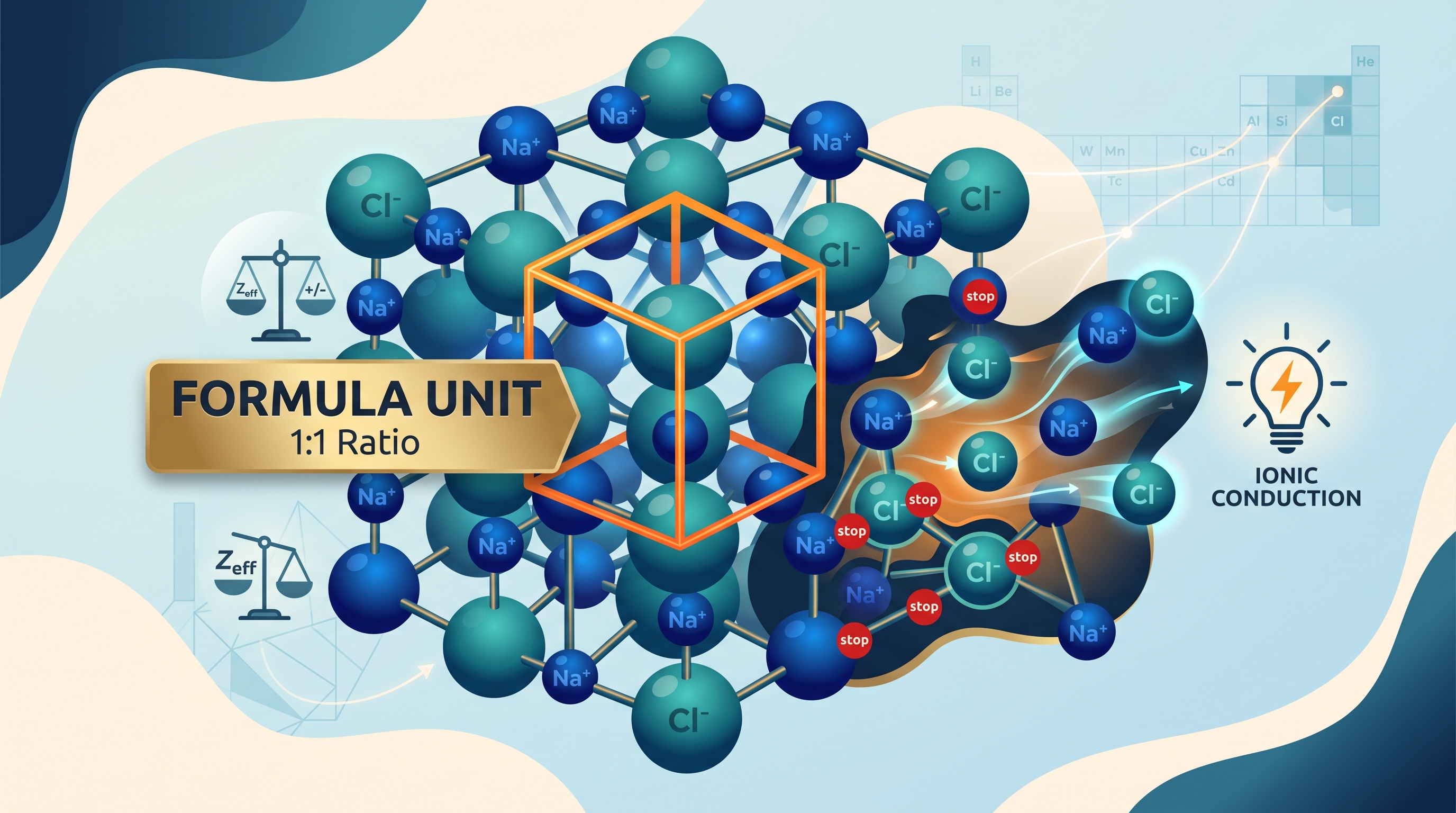
At the particulate level, $CaCl_2$ is an extended lattice of oppositely charged ions, not a collection of independent calcium-chlorine molecules. Strong Coulombic attractions throughout the lattice help explain its macroscopic properties: a high melting point, brittleness, and electrical conductivity when molten or dissolved because the ions can then move.
Misconception check: “Ionic compounds contain molecules”
A binary ionic compound contains two different elements, but its formula gives the lowest whole-number ratio of ions, not necessarily a discrete molecule. The formula unit $CaCl_2$ communicates the lattice’s $1:2$ ratio. Also, ionic solids do not conduct electricity well as solids because their ions are fixed in place; they conduct when molten or aqueous because the charged particles can move.
Science Practice 4: Model Analysis, skill code 4.A, asks students to predict or explain chemical properties or phenomena using theories, models, and representations. Here, the periodic table, shell model, Coulomb’s law, and ionic-lattice drawing work together: electron arrangement predicts charge; charge and distance predict attraction; attraction and lattice structure predict observable properties. This also develops the required connection between particulate-level structure and macroscopic behavior.
Retrieval check: Which atom should have the larger radius, sodium or chlorine, and why? Which ion is larger, $Na^+$ or $Cl^-$, and why? Finally, predict the formula of the compound formed by aluminum and oxygen. A strong answer should invoke shells, shielding, $Z_{\text{eff}}$, ionic charge, and charge neutrality rather than memorizing isolated formulas.

2.1 Types of Chemical Bonds · 2.2 Intramolecular Force and Potential Energy
Key concepts: Types of chemical bonds · Intramolecular forces · Potential energy versus internuclear distance · Equilibrium bond length · Bond energy · Covalent bond strength · Bond order · Sigma (σ) and pi (π) bonds · Coulombic forces · van der Waals forces
A chemical bond forms when attractive forces between particles outweigh repulsive forces at a particular separation. The result is not simply “atoms sticking together”: bond type, bond length, bond energy, and molecular behavior all emerge from the balance of electrostatic forces.
2.1 Types of Chemical Bonds · 2.2 Intramolecular Force and Potential Energy
A chemical bond forms when attractive forces between particles outweigh repulsive forces at a particular separation. The result is not simply “atoms sticking together”: bond type, bond length, bond energy, and molecular behavior all emerge from the balance of electrostatic forces.
The three major bond types
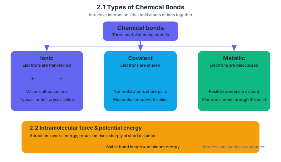
Chemical bonds are attractive interactions that hold atoms or ions together. The three broad types are ionic bonds, covalent bonds, and metallic bonds.
| Bond type | Particles involved | Electron behavior | Typical model |
|---|---|---|---|
| Ionic | Cations and anions | Electrons are transferred; oppositely charged ions attract | Extended crystal lattice |
| Covalent | Nonmetal atoms | Electrons are shared between atoms | Discrete molecules or network solids |
| Metallic | Metal atoms or cations | Valence electrons are delocalized throughout the solid | Positive centers in a mobile electron cloud |
Electronegativity and periodic trends help predict which bonding description is most useful. These categories are models rather than completely isolated boxes: a bond may have both ionic and covalent character, depending on how unevenly electrons are distributed.
Intramolecular versus intermolecular forces
Intramolecular forces act within a molecule or extended substance. Covalent bonds, such as the bonds inside a water molecule, are intramolecular forces. By contrast, intermolecular forces act between separate particles; van der Waals forces are examples of intermolecular attractions, not covalent bonds.
This distinction matters because breaking a covalent bond changes molecular identity, whereas overcoming an intermolecular attraction usually separates molecules without changing what each molecule is. Boiling water, for example, separates $H_2O$ molecules from one another but does not normally break the intramolecular $O-H$ bonds.
Key distinction: Intramolecular forces hold a chemical unit together; intermolecular forces hold separate chemical units near one another.
Potential energy and the distance between atoms
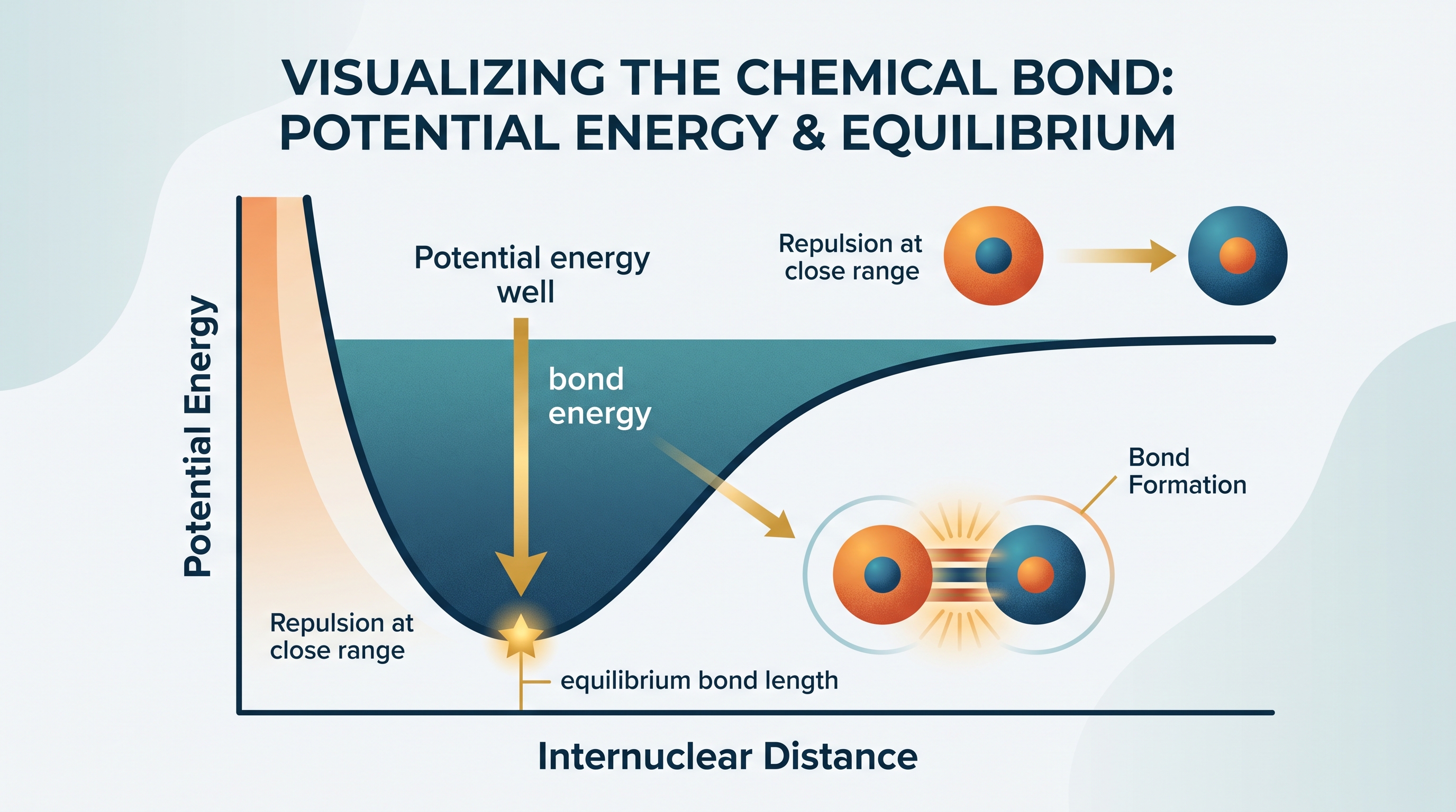
Imagine two atoms approaching like two magnets whose behavior changes dramatically with distance. At first, attraction lowers the system’s potential energy. If the atoms move too close, repulsions between nuclei and between occupied electron clouds rise sharply. The most stable distance is where these effects balance.
For a covalent bond, a graph of potential energy versus internuclear distance has a characteristic well:
The lowest point identifies the equilibrium bond length: the internuclear distance at which the bonded atoms have minimum potential energy. At this distance, the atoms are not motionless; they vibrate around the minimum.
The depth of the potential-energy well represents bond energy, the energy required to completely separate the bonded atoms. A deeper well corresponds to a stronger bond because more energy must be supplied to move the atoms from the bonded state to separated atoms.
$$ \text{bond energy} = E_{\text{separated atoms}}-E_{\text{bonded atoms}} $$
Worked example: If a covalent bond has an energy minimum at an internuclear distance of $120\ \mathrm{pm}$ and the energy of the separated atoms is $0\ \mathrm{kJ,mol^{-1}}$, while the minimum is $-460\ \mathrm{kJ,mol^{-1}}$, then the equilibrium bond length is $120\ \mathrm{pm}$ and the bond energy is $460\ \mathrm{kJ,mol^{-1}}$.
Misconception check — “closer always means stronger”: Moving atoms closer than the equilibrium distance does not strengthen the bond indefinitely. At very short distances, nucleus–nucleus and electron–electron repulsions make the potential energy increase.
Bond order, bond length, and bond strength
Bond order describes the number of shared electron pairs in a covalent bond: a single bond has order $1$, a double bond has order $2$, and a triple bond has order $3$. Increasing bond order generally concentrates more electron density between the nuclei, producing a shorter and stronger covalent bond.
The usual pattern is:
$$ \text{triple bond} > \text{double bond} > \text{single bond} $$
for bond energy, while the order reverses for bond length:
Atomic size also affects bond length. Larger bonded atoms have larger cores and generally place their nuclei farther apart, so their covalent bonds tend to be longer. Bond strength depends on the balance of attractive and repulsive Coulombic forces, not on distance alone.
Sigma and pi bonding
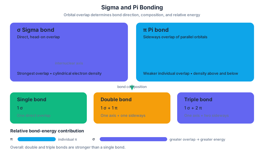
A sigma bond, written $\sigma$, forms from direct, head-on overlap of orbitals along the internuclear axis. A pi bond, written $\pi$, forms from sideways overlap of parallel orbitals above and below, or beside, that axis.
A single covalent bond contains one $\sigma$ bond. A double bond contains one $\sigma$ bond and one $\pi$ bond; a triple bond contains one $\sigma$ bond and two $\pi$ bonds.
The $\sigma$ bond has greater bond energy than an individual $\pi$ bond because head-on overlap is more effective than sideways overlap. Thus, a double bond is stronger overall than a single bond, but its additional $\pi$ bond is weaker than its $\sigma$ component.
AP science practices in this topic
This topic develops 3.A, Representing Data and Phenomena when you identify equilibrium bond length and bond energy from a potential-energy graph, and 3.B, Representing Data and Phenomena when you construct or annotate that graph. It develops 4.C, Model Analysis when you use the graph to explain why atoms attract at one distance and repel at another.
It also develops 6.A, Argumentation when you make a claim about relative bond strength and support it with bond order, atomic size, or energy-well depth, and 6.C, Argumentation when you refine that claim after comparing competing Coulombic attractions and repulsions.
Retrieval check: On a potential-energy graph, what does the horizontal coordinate of the minimum represent, and what does the vertical depth of the minimum represent? Why is a triple bond generally shorter and stronger than a single bond?
2.3 Structure of Ionic Solids · 2.4 Structure of Metals and Alloys
Key concepts: Structure of ionic solids · Structure of metals and alloys · Using visual models of atoms and ions to explain macroscopic properties · Relationship between particle structure and substance properties · Metallic bonding and the sea of mobile electrons · Electrical conductivity of metals and alloys · Alloys as mixtures of metals · Composition and properties of sterling silver · Tarnishing of metal alloys · Electrochemical cell voltage calculations
A crystal of table salt and a piece of copper can both look like ordinary solids, yet their particles are organized in fundamentally different ways: an ionic solid locks oppositely charged ions into a repeating lattice, while a metal places positive metal ions in a lattice surrounded by mobile, delocalized electrons.
2.3 Structure of Ionic Solids · 2.4 Structure of Metals and Alloys
A crystal of table salt and a piece of copper can both look like ordinary solids, yet their particles are organized in fundamentally different ways: an ionic solid locks oppositely charged ions into a repeating lattice, while a metal places positive metal ions in a lattice surrounded by mobile, delocalized electrons. Those microscopic models explain why salt crystals fracture but copper can be bent, and why solid salt does not conduct electricity while copper does.
Ionic solids: an organized three-dimensional lattice
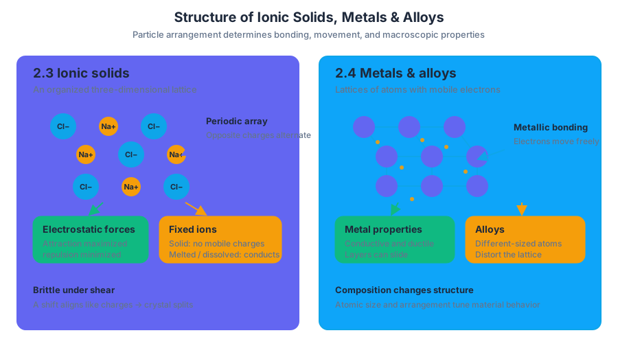
Learning Objective 2.3.A requires students to represent an ionic solid with a particulate model consistent with Coulomb’s law and the properties of its constituent ions. In an ionic crystal, cations and anions occupy a systematic, periodic three-dimensional array. The arrangement maximizes attractive interactions between opposite charges while minimizing repulsive interactions between like charges.
Essential Knowledge 2.3.A.1: The cations and anions in an ionic crystal are arranged in a systematic, periodic 3-D array that maximizes the attractive forces among cations and anions while minimizing the repulsive forces.
A useful model of sodium chloride is not a collection of separate sodium chloride molecules. Instead, it is an extended pattern in which each $Na^+$ ion is surrounded by nearby $Cl^-$ ions, and each $Cl^-$ ion is surrounded by nearby $Na^+$ ions. The model must show both charge and relative particle size: changing an ion’s charge or radius changes the distances and strengths of the electrostatic interactions.
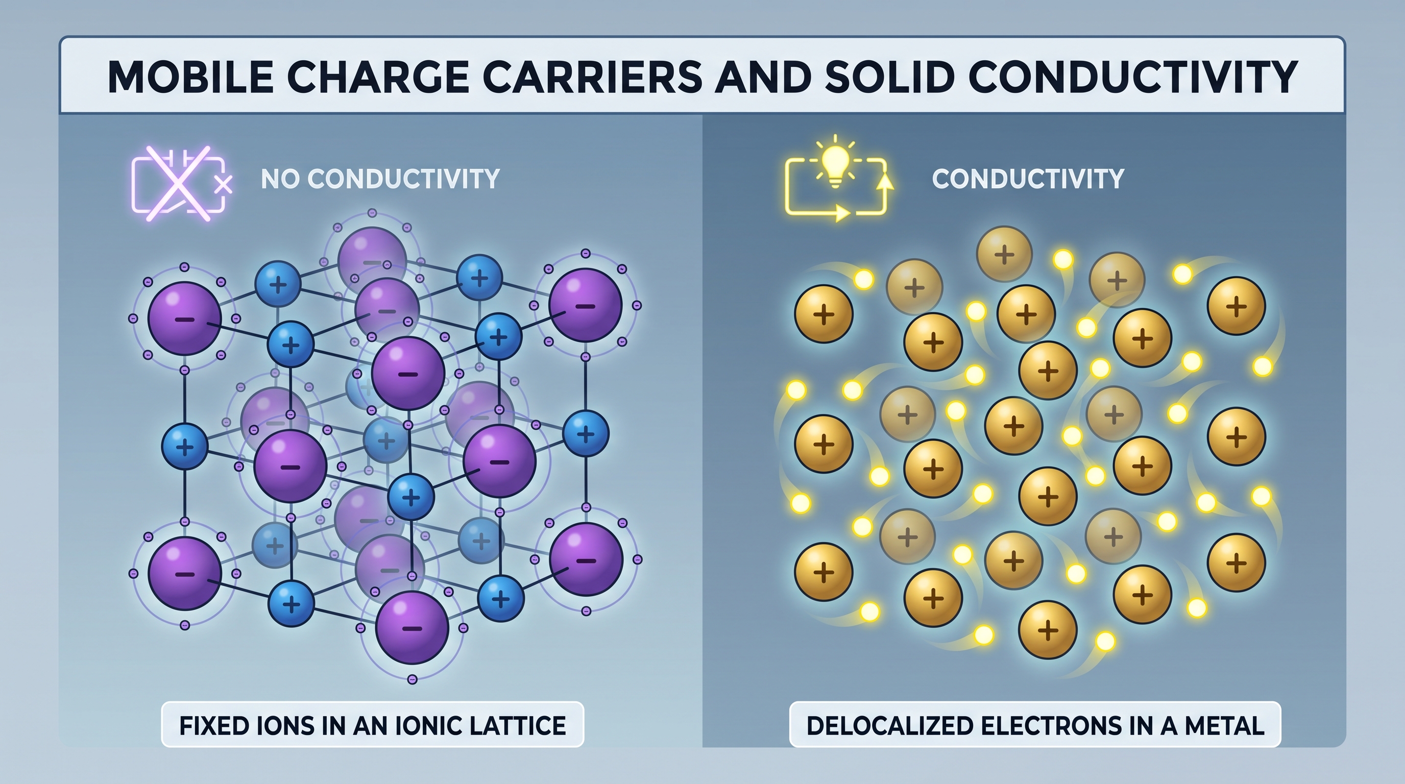
The lattice model predicts macroscopic properties. Because the ions are held in fixed positions, a solid ionic crystal generally does not conduct electricity: its charged particles cannot move through the solid. If the crystal melts or dissolves in water, ions can move, so the material can conduct. Ionic solids are also often brittle. When a layer of ions shifts, like charges may become aligned beside one another; strong repulsion then causes the crystal to split rather than deform smoothly.
Worked model-analysis example
Imagine comparing two diagrams. Model A shows alternating positive and negative ions in a repeating array. Model B shows positive ions clustered beside positive ions, with negative ions clustered elsewhere. Model A is consistent with 2.3.A.1 because it maximizes cation–anion attraction and reduces cation–cation and anion–anion repulsion. Model B is not a plausible stable ionic crystal, even if its total numbers of positive and negative charges are correct.
The exam-relevant reasoning is Science Practice 4: Model Analysis, specifically 4.C Explain the connection between particulate-level and macroscopic properties of a substance using models and representations. Do not merely identify the lattice; use it to explain an observation: fixed ions account for poor solid-state conductivity, and the periodic arrangement of strong attractions accounts for a rigid crystal structure.
Metals: positive ions in a sea of electrons
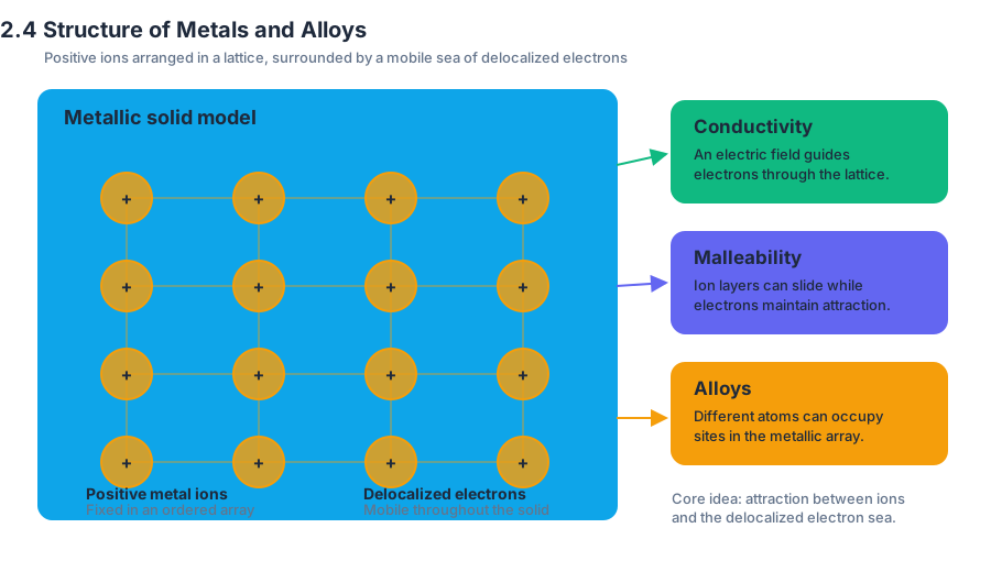
Learning Objective 2.4.A requires students to represent a metallic solid and/or alloy using a model that shows the essential characteristics of its structure and interactions. In the metallic-bonding model, positive metal ions form an array while valence electrons are delocalized, meaning they are not assigned to one particular atom. They move throughout the solid as a mobile “sea of electrons.”
Essential Knowledge 2.4.A.1: Metallic bonding can be represented as an array of positive metal ions surrounded by delocalized valence electrons, or a “sea of electrons.”
The mobile electrons explain why metals conduct electricity: when an electric field is applied, the electrons can move through the lattice and carry charge. The same model helps explain malleability and ductility. If layers of metal ions slide, the delocalized electrons continue to attract the positive ions, so the structure can change shape without the entire lattice shattering.
Alloys: changing the lattice without eliminating electron mobility
An alloy is a metallic solid containing atoms of more than one element. Its properties depend strongly on how the different-sized atoms fit into the metal lattice.
An interstitial alloy forms when much smaller atoms occupy spaces between larger metal atoms. In steel, carbon atoms occupy interstitial spaces in an iron lattice. These smaller atoms obstruct the movement of iron layers, so the alloy is typically harder and less easily deformed than pure iron.
Essential Knowledge 2.4.A.2: Interstitial alloys form between atoms of significantly different radii, where the smaller atoms fill the interstitial spaces between the larger atoms, as in carbon in iron.
A substitutional alloy forms when atoms of comparable radius replace some of the original atoms in the lattice. In certain brass alloys, zinc atoms substitute for copper atoms. The substitutions distort the regular lattice and can increase strength while preserving the delocalized-electron model, so the alloy generally remains electrically conducting.
Essential Knowledge 2.4.A.3: Substitutional alloys form between atoms of comparable radius, where one atom substitutes for the other in the lattice, as in zinc substituting for copper in certain brass alloys.
Sterling silver illustrates a substitutional-alloy context: it contains $92.5%$ silver and $7.5%$ other metals, such as copper, by mass. It remains metallic and conducts electricity, but its altered lattice gives it greater durability than pure silver. Over time, sterling silver can tarnish because surface atoms undergo chemical reactions with substances in the environment; conductivity and metallic structure do not mean that the surface is chemically unreactive.
Misconception check
Misconception: “All solids conduct because their particles contain electrons.” Conductivity requires mobile charge carriers, not merely charged particles or electrons somewhere inside atoms. In a solid ionic crystal, ions are present but fixed; in a metal or metallic alloy, delocalized electrons can move through the structure.
Retrieval check: Which model best explains each observation: an ionic lattice, a pure-metal lattice, an interstitial alloy, or a substitutional alloy?
- A crystal fractures when layers shift.
- A solid conducts electricity and can be drawn into wire.
- Carbon makes iron harder.
- Zinc replaces copper atoms in brass.
Answers: $1$ is an ionic lattice, $2$ is a pure-metal lattice, $3$ is an interstitial alloy, and $4$ is a substitutional alloy. In every case, the strongest explanation begins with the particle model and ends with the observable property.
2.5 Lewis Diagrams · 2.6 Resonance and Formal Charge
Key concepts: Lewis diagrams · Resonance and formal charge · Octet rule · Formal charge as a structure-selection criterion · Limitations of the Lewis structure model · VSEPR theory · Bond orders · Bond polarities · Molecular structure and properties · Valence electrons
A Lewis diagram represents valence electrons as bonding pairs and nonbonding pairs, turning invisible electron arrangements into a model that can predict molecular structure and properties.
2.5 Lewis Diagrams · 2.6 Resonance and Formal Charge
A Lewis diagram represents valence electrons as bonding pairs and nonbonding pairs, turning invisible electron arrangements into a model that can predict molecular structure and properties. The key question is not merely “Can this structure be drawn?” but “Which drawing best represents the electron distribution?”
Building a Lewis diagram
A bonding pair is shown as a line between atoms; a lone pair is a pair of valence electrons located on one atom and not shared in a bond. The octet rule states that many main-group atoms are especially stable when surrounded by eight valence electrons, although hydrogen follows a duet rule and some atoms, such as aluminum, can be electron-deficient.
To construct a Lewis diagram, count the total valence electrons, select a reasonable skeletal arrangement, connect atoms with single bonds, complete terminal-atom octets, place remaining electrons on the central atom, and create multiple bonds if the central atom lacks an octet. For an ion, add electrons for a negative charge and remove electrons for a positive charge.
Worked example: nitrate, $NO_3^-$
Count valence electrons:
$$ 5+3(6)+1=24\text{ electrons} $$
Place nitrogen in the center and connect it to three oxygen atoms with single bonds. Those bonds use $6$ electrons. Completing the three oxygen octets uses $18$ additional electrons, leaving no electrons for nitrogen’s octet. Convert one oxygen lone pair into a second $N-O$ bond. Nitrogen now has an octet, and the structure contains one $N=O$ bond and two $N-O^-$ bonds.
The formal charge of an atom is the charge it would have if bonding electrons were divided equally:
$$ \text{Formal charge}
V-\left(N+\frac{B}{2}\right) $$
Here, $V$ is the atom’s valence-electron count, $N$ is its number of nonbonding electrons, and $B$ is the number of bonding electrons. In one nitrate contributor, the double-bonded oxygen has formal charge $0$, the two single-bonded oxygens each have formal charge $-1$, and nitrogen has formal charge $+1$. The total is $-1$, matching the ion’s charge.
Resonance: several drawings, one delocalized structure
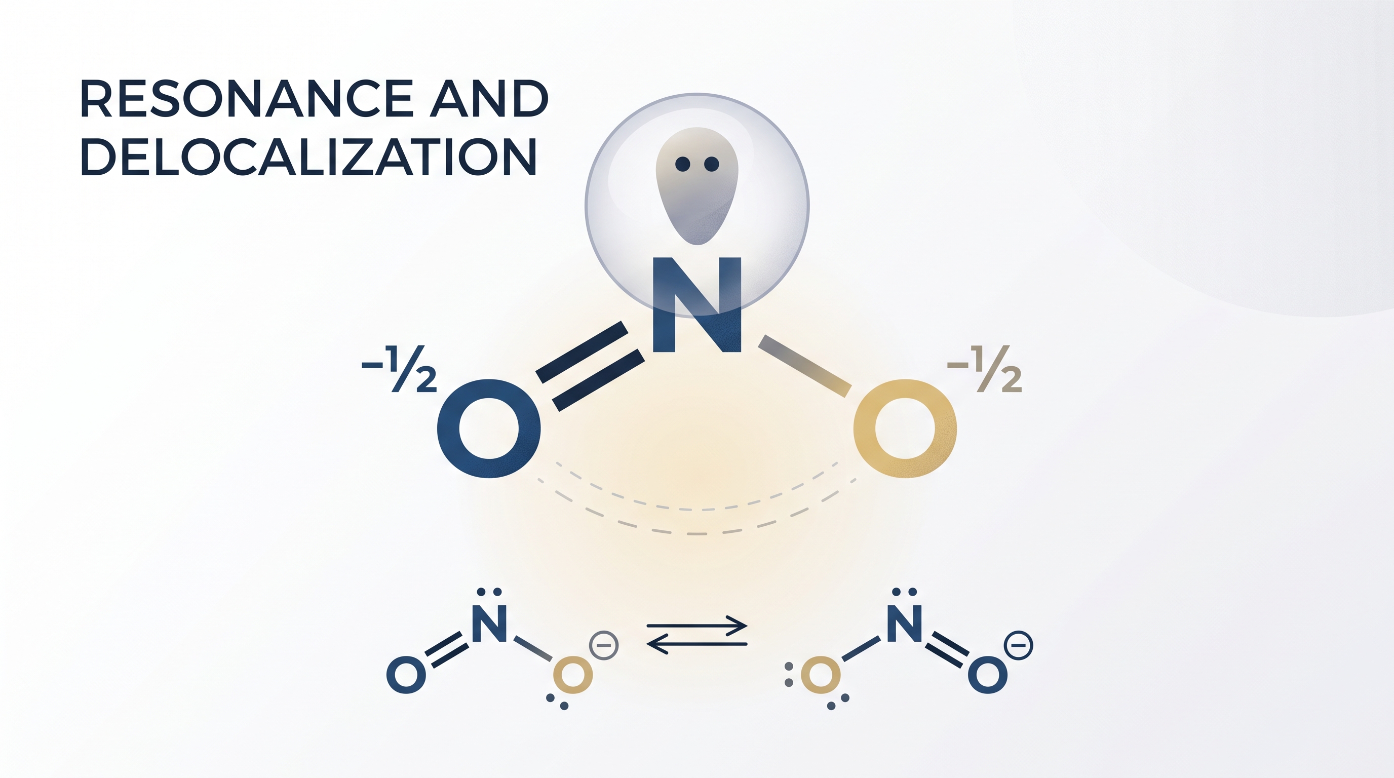
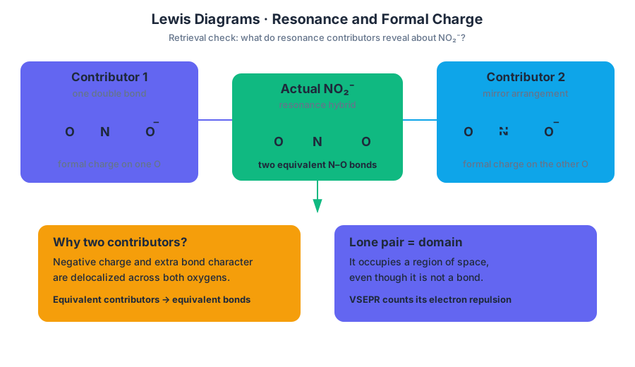
When equivalent Lewis diagrams differ only in the location of a multiple bond or charge, they are resonance structures. The molecule does not rapidly switch between these drawings. Instead, the actual electron distribution is a resonance hybrid in which electrons are delocalized over multiple atoms.
Nitrate has three equivalent resonance structures because the $N=O$ bond can be placed to any one of the three oxygen atoms. Consequently, all three $N-O$ bonds are equivalent in the real ion, with an average bond order of approximately
$$ \frac{4}{3} $$
This refinement is required by 2.6.A.1: resonance often gives qualitatively more accurate predictions of molecular structure and properties than any single Lewis contributor. Curved arrows may show electron movement between contributors, but the atoms themselves do not move.
Choosing among nonequivalent structures
Resonance contributors are not always equivalent. When possible structures differ in formal-charge placement, use the octet rule and formal charge together, as required by 2.6.A.2.
A strong candidate generally:
- gives main-group atoms complete octets when reasonable;
- minimizes the magnitude and number of formal charges;
- places negative formal charge on the more electronegative atom;
- avoids unnecessary charge separation.
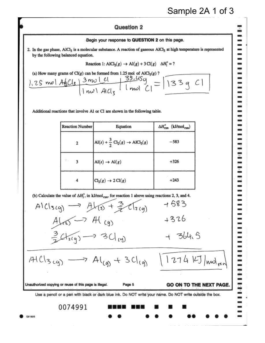
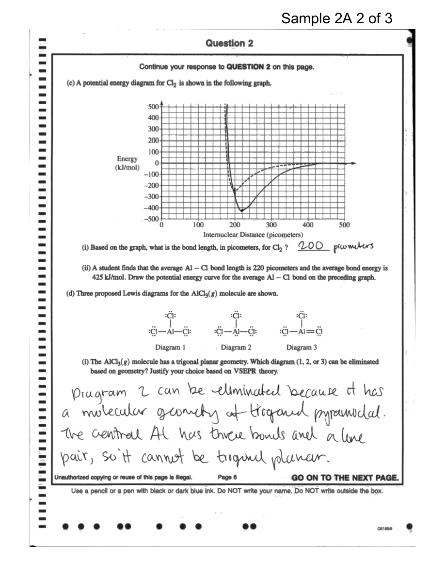
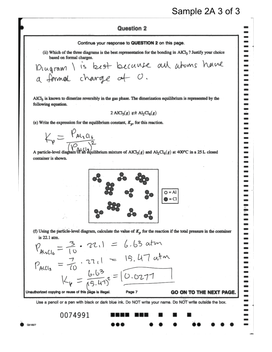
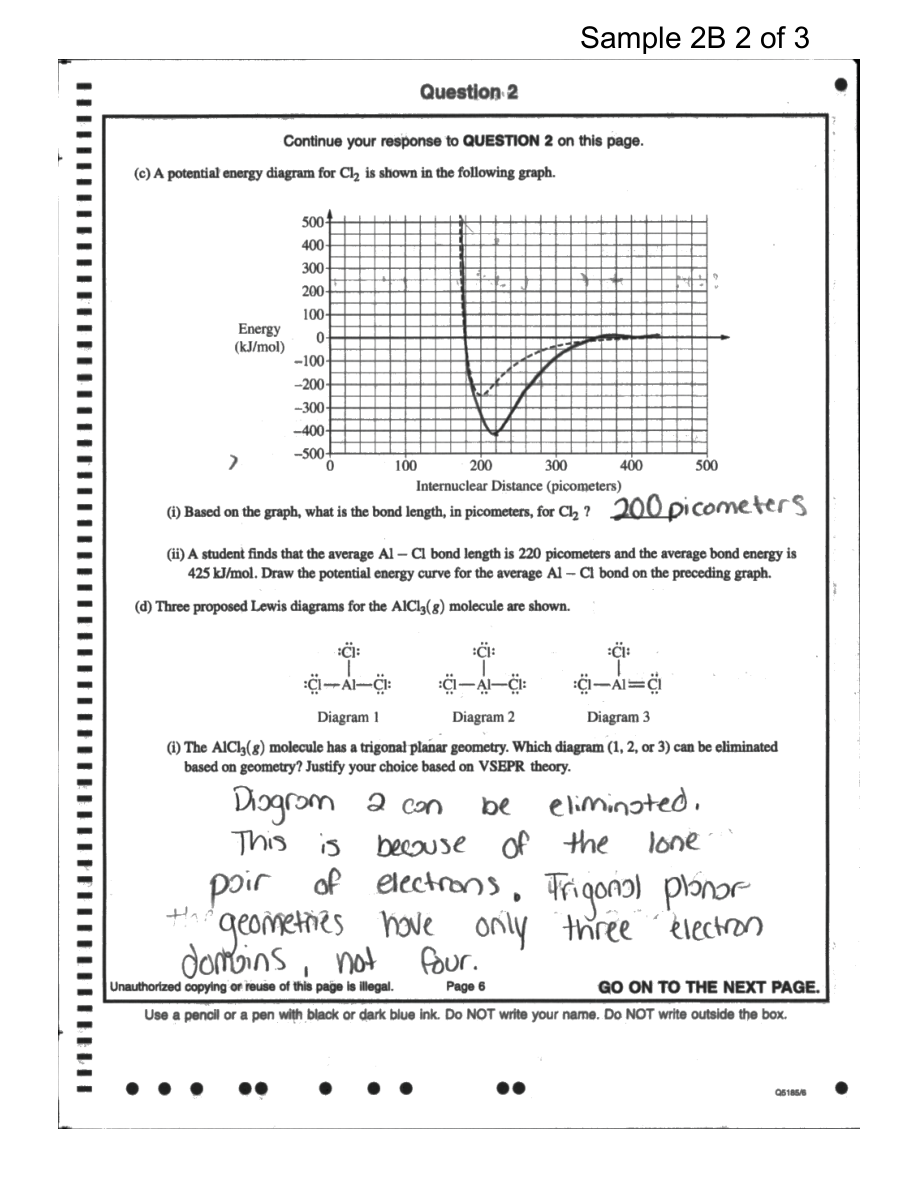
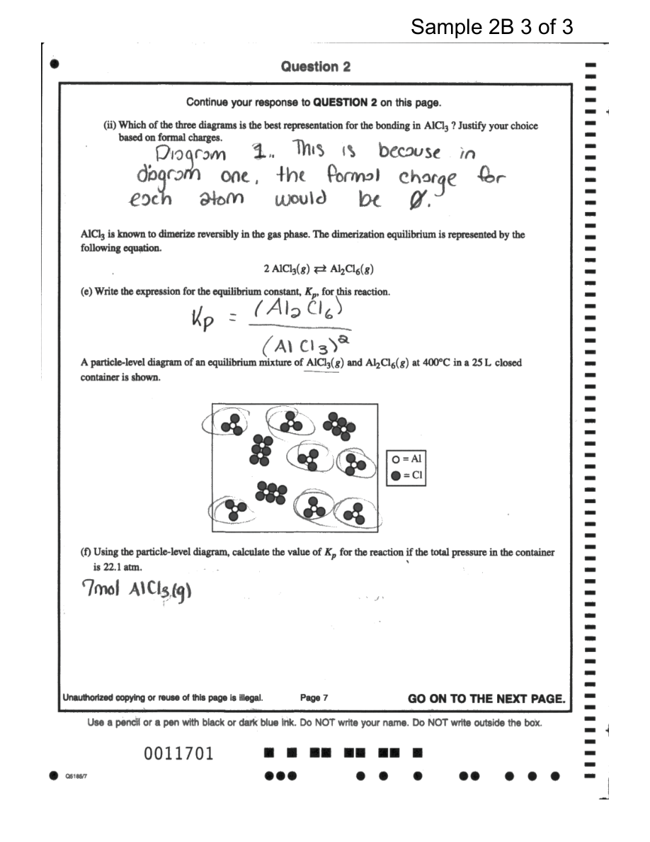
These are criteria, not absolute laws. A structure with an incomplete octet can be the better model when the central atom is electron-deficient, as in gaseous $AlCl_3$. A trigonal-planar $AlCl_3$ molecule has three bonding electron domains around aluminum. A proposed diagram containing an aluminum lone pair would create four electron domains and therefore cannot match that geometry.
Lewis diagrams and VSEPR
VSEPR theory, or Valence Shell Electron Pair Repulsion theory, predicts that electron domains around a central atom arrange themselves as far apart as possible because electron regions repel one another. A single bond, double bond, triple bond, or lone pair each counts as one electron domain; lone pairs usually repel more strongly than bonding pairs.
Lewis diagrams therefore provide the electron-domain count used for a first qualitative geometry prediction. For $AlCl_3$, three bonding domains and no lone pairs suggest a trigonal-planar arrangement. Detailed molecular shapes and hybridization follow from this electron-domain analysis, but the essential connection is simple: Lewis diagrams show the domains; VSEPR explains their spatial arrangement.
Bond polarity and model limitations
A polar bond forms when bonded atoms have unequal electronegativities. The more electronegative atom attracts shared electrons more strongly and becomes partially negative, written $\delta^-$; the other becomes partially positive, written $\delta^+$. Formal charges describe an idealized whole-number electron accounting, whereas partial charges describe unequal sharing.
Resonance can spread charge and bond character across several atoms. In nitrate, no single oxygen permanently carries the double bond or the entire negative-charge pattern; the delocalized distribution makes the three bonds equivalent and influences the ion’s polarity. Molecular polarity also depends on whether individual bond dipoles cancel through the molecule’s geometry.
Lewis structures are models, not photographs of electron density. They work especially well for counting valence electrons, identifying bonding and lone pairs, and making qualitative predictions, but they cannot represent delocalization perfectly. Their limitations are especially important for species with an odd number of valence electrons, because one electron cannot be paired into a conventional octet; such species are commonly described as radicals. This limitation is specified by 2.6.A.3.
AP science practices in action
This topic most directly develops Science Practice 1: Models and Representations, by constructing and revising Lewis diagrams; Science Practice 4: Model Analysis, by judging octet completion, resonance, formal charge, and model limitations; and Science Practice 6: Argumentation, by using those features as evidence for a structural claim. It also uses Science Practice 5: Mathematical Routines when counting valence electrons or calculating formal charge.
The official learning objective is 2.6.A: “Represent a molecule with a Lewis diagram that accounts for resonance between equivalent structures or that uses formal charge to select between nonequivalent structures.” A complete scientific argument should therefore state a claim, cite the relevant Lewis or VSEPR evidence, and explain why that evidence supports the predicted structure or property.
Retrieval check
For $NO_2^-$, predict how many equivalent resonance contributors are possible and explain why the two $N-O$ bonds are equivalent in the actual ion. Then answer: why does a lone pair count as an electron domain even though it is not a bond?
Check: There are two equivalent contributors, so the negative charge and extra bond character are delocalized across both oxygens; the actual $N-O$ bonds are equivalent. A lone pair occupies a region of space and repels other electron regions, so VSEPR counts it as one electron domain.
2.7 VSEPR and Hybridization
Key concepts: VSEPR theory and its use in explaining molecular shapes · Hybridization nomenclature: sp, sp2, and sp3 · Approximate bond angles associated with molecular geometries · Dimensional analysis as a self-correction tool in calculations · Checking that final units match the requested units, such as kJ
A molecule’s shape is not decoration: it determines which atoms can approach one another, how bonds are oriented, and often how the substance reacts. VSEPR theory—Valence Shell Electron-Pair Repulsion theory—explains molecular shape by treating electron domains around a central atom as charged regions that spread…
2.7 VSEPR and Hybridization
A molecule’s shape is not decoration: it determines which atoms can approach one another, how bonds are oriented, and often how the substance reacts. VSEPR theory—Valence Shell Electron-Pair Repulsion theory—explains molecular shape by treating electron domains around a central atom as charged regions that spread out to minimize repulsion.
From electron domains to molecular geometry
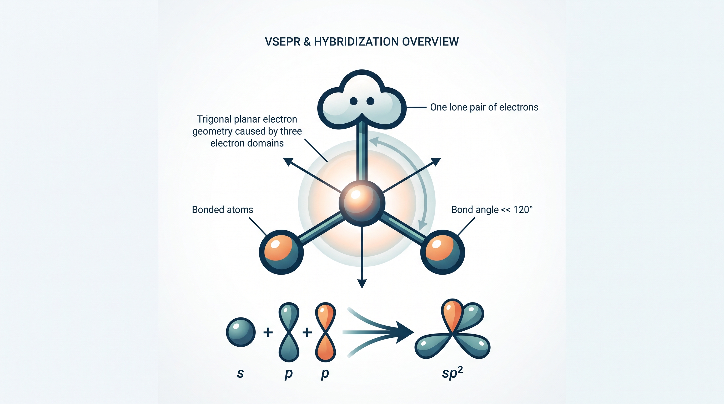
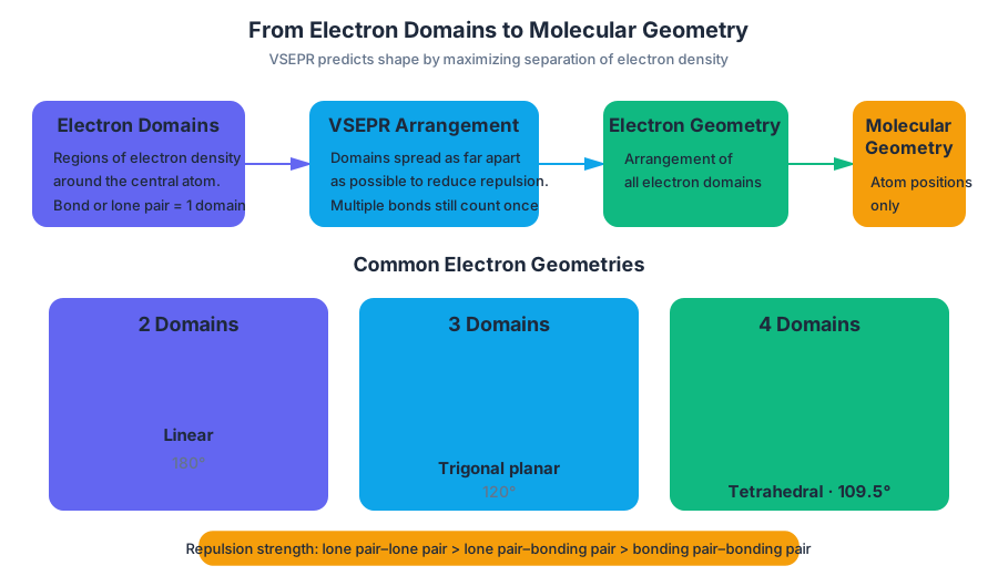
An electron domain is a region of electron density around the central atom. A single bond, double bond, triple bond, lone pair, or unpaired electron counts as one domain. A multiple bond contains more electrons than a single bond, but it still occupies one overall direction in the VSEPR model.
The electron domains arrange themselves as far apart as possible. The resulting electron geometry describes the arrangement of all domains, while the molecular geometry describes only the positions of the atoms. Lone pairs affect the arrangement even though they are not included in the name of the molecular shape.
| Electron domains around central atom | Electron geometry | Approximate bond angle |
|---|---|---|
| $2$ | Linear | $180^\circ$ |
| $3$ | Trigonal planar | $120^\circ$ |
| $4$ | Tetrahedral | $109.5^\circ$ |
Repulsions are not equally strong. Lone pair–lone pair repulsion is stronger than lone pair–bonding pair repulsion, which is stronger than bonding pair–bonding pair repulsion. Therefore, lone pairs compress nearby bond angles.
Worked molecular-shape example: nitrogen oxides
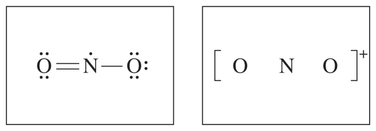
In $NO_2$, the nitrogen has approximately three electron domains: two bonding regions and one region associated with the unpaired electron. The arrangement is approximately trigonal planar, so the nitrogen is described with $sp^2$ hybridization and the bond angle is approximately $120^\circ$.
In $NO_2^+$, nitrogen has two bonding domains and no lone pair. The domains move opposite each other, giving a linear molecular geometry. Nitrogen is therefore described with $sp$ hybridization, and the bond angle is approximately $180^\circ$.
Key distinction: Count electron domains around the central atom—not the number of lines in a structural formula and not the number of atoms in the molecule.
Hybridization nomenclature
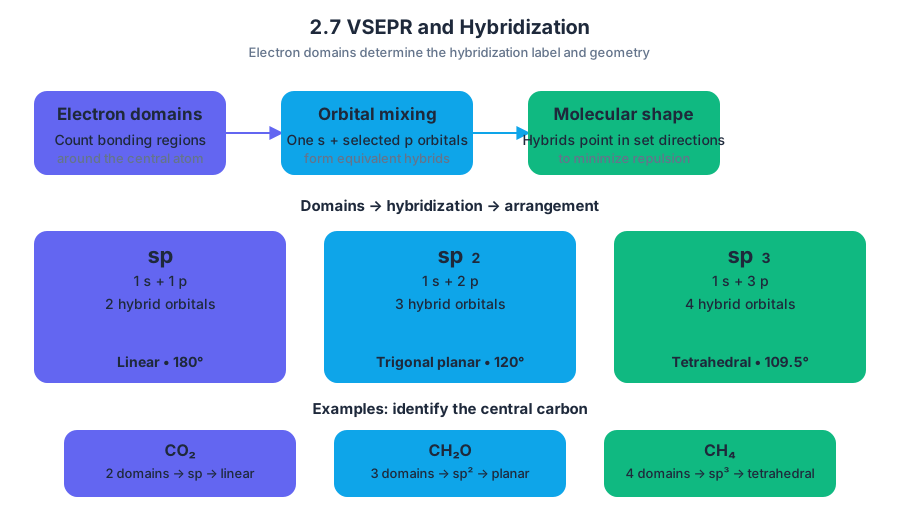
Hybridization is a model in which atomic orbitals combine to produce a set of equivalent hybrid orbitals oriented in particular directions. The notation names the orbitals mixed: $s$ for an $s$ orbital and $p$ for a $p$ orbital.
For the hybridization nomenclature assessed here:
- $sp$ means one $s$ orbital combines with one $p$ orbital, producing two hybrid orbitals and a linear arrangement.
- $sp^2$ means one $s$ orbital combines with two $p$ orbitals, producing three hybrid orbitals and a trigonal-planar arrangement.
- $sp^3$ means one $s$ orbital combines with three $p$ orbitals, producing four hybrid orbitals and a tetrahedral electron arrangement.
The hybridization label follows the number of electron domains:
$$ \text{number of electron domains} \longrightarrow \text{hybridization} $$
$$ 2 \longrightarrow sp,\qquad 3 \longrightarrow sp^2,\qquad 4 \longrightarrow sp^3 $$
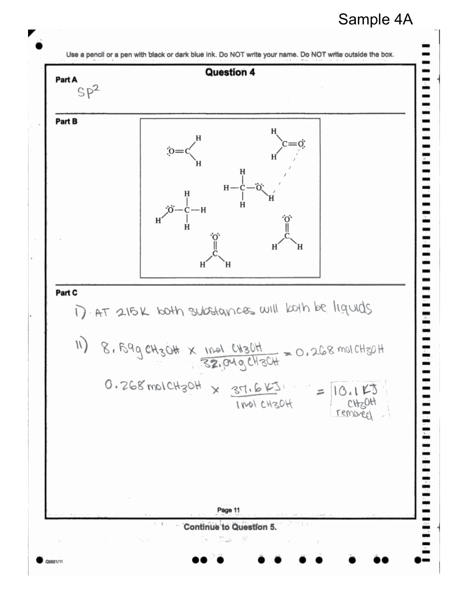
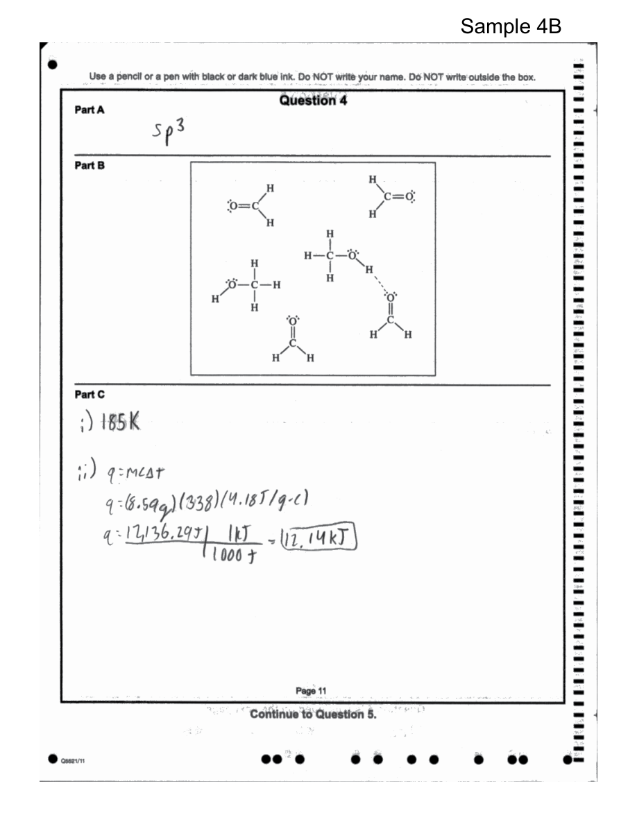
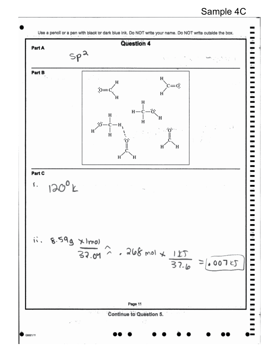
For example, the central carbon in $CO_2$ has two bonding domains, so it is $sp$ hybridized and linear. The central carbon in $CH_2O$ has three electron domains—two $C-H$ bonds and one $C=O$ bond—so it is $sp^2$ hybridized and approximately trigonal planar. A carbon atom with four single-bonding domains, such as the carbon in $CH_4$, is $sp^3$ hybridized and tetrahedral.
Misconception check
Misconception: a double bond counts as two electron domains. It does not. The entire double bond points in one direction and therefore counts as one domain for VSEPR. The same rule applies to a triple bond.
Misconception: hybridization is the same as electron configuration. Electron configuration describes how electrons occupy atomic orbitals. Hybridization is a bonding-and-shape model used to describe the directions of orbitals involved in bonding. Do not assign $sp^3$ merely because an atom has four valence electrons; assign it when the central atom has four electron domains.
Hybridization involving $d$ orbitals is outside the assessed scope here. For the required cases, stop at $sp$, $sp^2$, and $sp^3$.
Dimensional analysis: the unit check that catches bad chemistry
Dimensional analysis tracks units through a calculation. It is a self-correction tool: if the requested quantity is energy, the final units must be energy units such as $\text{kJ}$.
Suppose a molecular-energy calculation gives a molar enthalpy change of $40.4\ \text{kJ mol}^{-1}$ for $0.250\ \text{mol}$ of a substance:
$$ 0.250\ \text{mol} \left( \frac{40.4\ \text{kJ}}{1\ \text{mol}} \right)
10.1\ \text{kJ} $$
The $\text{mol}$ units cancel, leaving $\text{kJ}$, exactly as required. If a proposed setup ended in $\text{mol}$, $\text{K}$, or $\text{kJ mol}^{-1}$, the calculation would be fundamentally mismatched to the question—even if the numerical value looked reasonable.
Retrieval check
A central atom has three electron domains: two bonds and one lone pair. Predict its electron geometry, approximate bond angle, and hybridization. Then explain why a double bond would still count as only one domain. Finally, if an energy calculation is requested in $\text{kJ}$, identify the unit that must appear after all conversion factors cancel.
3.1 Intermolecular and Interparticle Forces · 3.2 Properties of Solids
Key concepts: Intermolecular forces and macroscopic properties · London dispersion forces · Dipole-induced dipole interactions · Molecular polarity and polarizability · Relative strength of intermolecular forces · Solubility and intermolecular interactions · Covalent network solids · Three-dimensional and two-dimensional covalent networks · Macroscopic properties of solids · Chromatography as evidence of polarity
A liquid’s boiling point, a dye’s movement through paper, and graphite’s surprising softness all arise from how particles attract one another. Intermolecular forces are attractions between separate molecules; interparticle forces is the broader term, including attractions between atoms, ions, and molecules.
3.1 Intermolecular and Interparticle Forces · 3.2 Properties of Solids
A liquid’s boiling point, a dye’s movement through paper, and graphite’s surprising softness all arise from how particles attract one another. Intermolecular forces are attractions between separate molecules; interparticle forces is the broader term, including attractions between atoms, ions, and molecules.
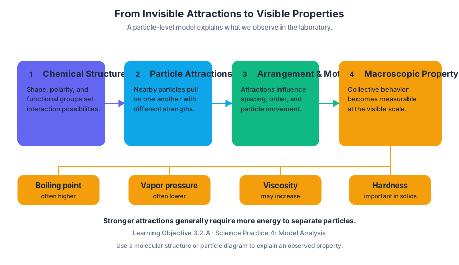
From invisible attractions to visible properties
A molecule’s structure determines how strongly it interacts with nearby particles. Stronger attractions generally require more energy to separate particles, so they can produce higher boiling points, lower vapor pressures, greater viscosity, or greater hardness in a solid.
The central reasoning chain is:
$$ \text{chemical structure} \longrightarrow \text{particle attractions} \longrightarrow \text{particle arrangement and motion} \longrightarrow \text{macroscopic property} $$
This is the focus of Learning Objective 3.2.A: explain the relationship among a substance’s macroscopic properties, its particulate-level structure, and the interactions between its particles. In AP Chemistry, this connection is developed through Science Practice 4: Model Analysis, especially when a particle diagram or molecular structure must explain an observed property.
London dispersion forces
London dispersion forces are attractions caused by temporary, fluctuating dipoles. Even a nonpolar molecule has electrons that move constantly; for an instant, the electron cloud may be more concentrated on one side, creating a temporary partial negative end and a temporary partial positive end in the same molecule. That temporary dipole can distort a neighboring electron cloud and induce an opposite dipole.
According to Essential Knowledge 3.1.A.1, London dispersion forces result from Coulombic interactions between temporary, fluctuating dipoles and are always attractive. They occur between nonpolar molecules, polar molecules, and mixtures containing both.
The ease with which an electron cloud can be distorted is called polarizability. Larger particles with more electrons are usually more polarizable. Molecular shape also matters: elongated molecules can have greater surface-to-surface contact than compact molecules, increasing the total attraction.
Misconception check — “Nonpolar means no attractions.” Nonpolar molecules have no permanent dipole, but they still experience London dispersion forces. A sample of nonpolar molecules can condense because temporary dipoles continually attract neighboring particles.
Dipole-induced dipole interactions and polarity
A dipole-induced dipole interaction occurs when a polar molecule approaches a nonpolar molecule. The polar molecule’s permanent dipole distorts the nonpolar molecule’s electron cloud, producing an induced dipole. The attraction becomes stronger as the polar molecule’s dipole magnitude increases and as the nonpolar molecule becomes more polarizable.
Polar molecules also experience dipole-dipole attractions. These depend on both dipole magnitude and orientation: opposite partial charges attract, while similarly charged ends repel. Polar molecules of comparable size usually attract more strongly than nonpolar molecules because dipole-dipole interactions act in addition to London dispersion forces.
Other important attractions include ion-dipole forces, between an ion and a polar molecule, and hydrogen bonding, a particularly strong interaction in which hydrogen covalently bonded to nitrogen, oxygen, or fluorine is attracted to a nearby electronegative atom. These interactions are relevant to Essential Knowledge 3.1.A.3 and 3.1.A.4.
When comparing forces, first ask whether the particles are the same chemical species or different species, as required by Learning Objective 3.1.A. For molecules of the same species, compare size, electron count, shape, and polarizability. For different species, identify all applicable interactions rather than assigning a single force automatically.
Worked example: why a larger nonpolar molecule can boil at a higher temperature
Compare two nonpolar molecules with similar shapes: one has fewer electrons, and the other has many more. Neither has permanent dipole-dipole attractions, but the larger molecule has a more polarizable electron cloud. Its London dispersion forces are stronger, so more energy is required to separate its molecules. The larger molecule therefore tends to have the higher boiling point and lower vapor pressure.
Solubility: separating old attractions and forming new ones
Solubility describes how much of one substance dissolves in another. Dissolving is not simply “particles disappearing”; it requires breaking attractions among solute particles and solvent particles, then forming new solute-solvent attractions.
$$ \text{net dissolving tendency} \sim \text{new solute-solvent attractions}
\text{interactions that must be disrupted} $$
A polar solvent tends to interact favorably with polar solutes through dipole-dipole, hydrogen-bonding, or ion-dipole attractions. A nonpolar solvent tends to dissolve nonpolar substances through London dispersion forces. This is the molecular meaning behind the useful pattern “like dissolves like,” although solubility depends on the balance of all interactions involved.
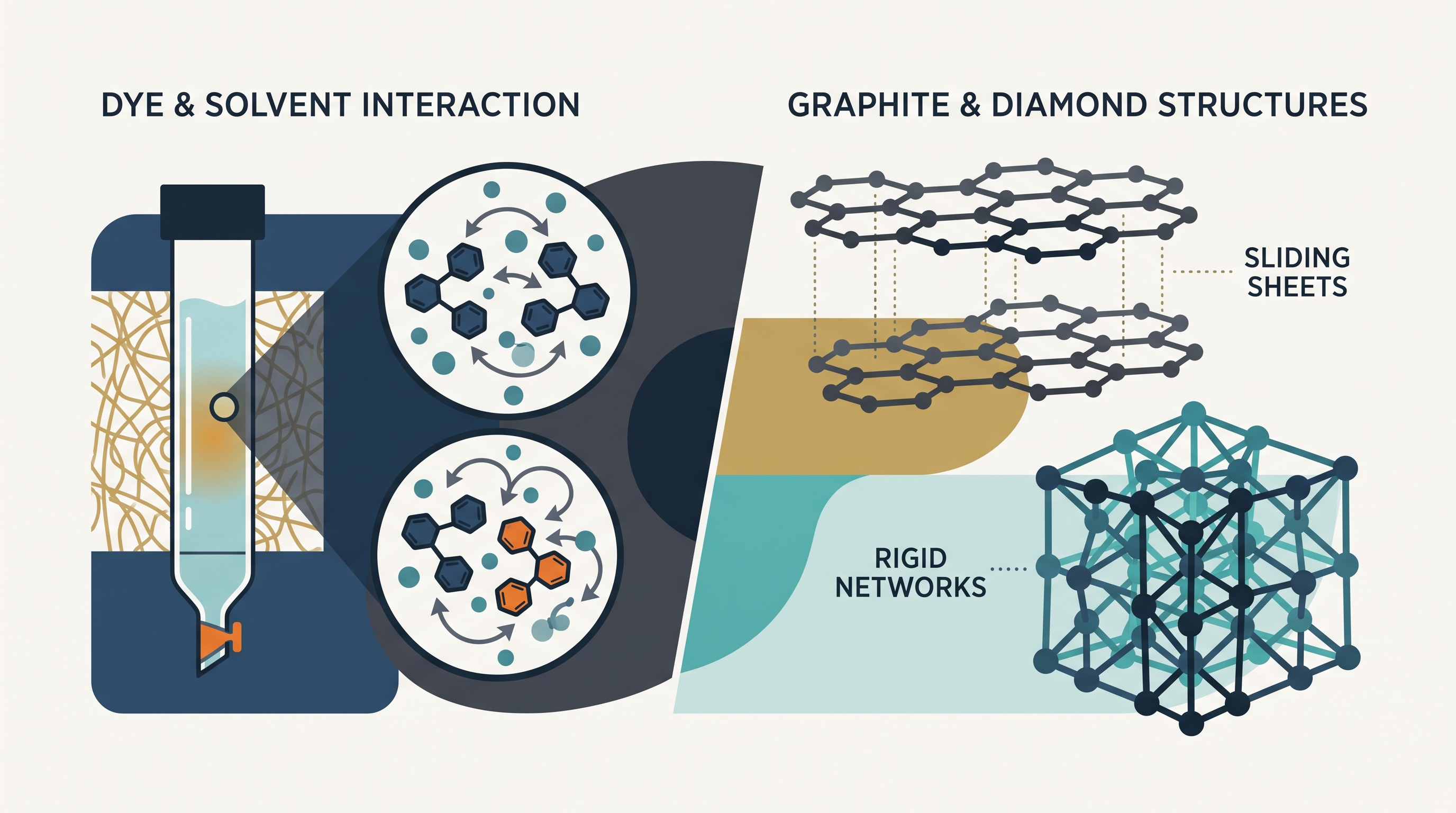
Chromatography provides a visible polarity test. As a solvent moves across paper, different dyes repeatedly partition between the mobile solvent and the stationary paper. A dye that interacts more strongly with the solvent travels farther; a dye that interacts more strongly with the paper travels less. Comparing the distances can identify which dye is most polar relative to that solvent-paper system.
Covalent network solids
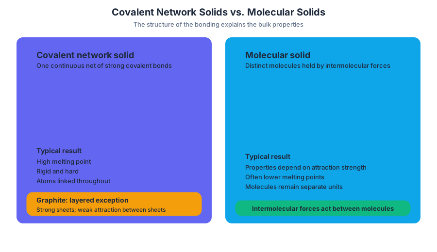
A covalent network solid consists of atoms joined by covalent bonds throughout an extended structure rather than separate molecules held together only by intermolecular forces. The network may extend in three dimensions, as in diamond, or in two-dimensional layers, as in graphite.
Essential Knowledge 3.2.A.4 identifies covalent network solids as structures formed from nonmetals and metalloids, either as elements or as binary compounds such as silicon dioxide and silicon carbide. Because strong covalent bonds connect atoms across the network, these substances generally have high melting points and are rigid and hard.
Graphite is the essential structural exception. Each layer contains strong covalent bonds, but the attraction between adjacent layers is much weaker, allowing the layers to slide past one another relatively easily. Pencil “lead” marks paper because graphite layers shear away, even though each individual layer is strongly bonded.
By contrast, Essential Knowledge 3.2.A.5 describes molecular solids as collections of distinct molecules held together between molecules by intermolecular forces. Their bulk properties therefore depend strongly on the strength of those intermolecular attractions, rather than on one continuous covalent network.
In-flow retrieval check
A nonpolar dye travels farther in a particular chromatography solvent than a polar dye. Which interaction is probably stronger for the traveling dye: dye-paper or dye-solvent? Answer: dye-solvent. The dye is spending more time associated with the mobile solvent, so it moves farther. Explain the same result at the particulate level, then predict why graphite can be soft while diamond is hard.
3.3 Solids, Liquids, and Gases · 3.4 Ideal Gas Law
Key concepts: Particulate-level differences among solids, liquids, and gases · Noncovalent interparticle interactions · Macroscopic properties of ideal gases · The ideal gas law · Relationships among pressure, volume, amount, and temperature · Gas mixtures and partial pressures · Non-ideal gas behavior · Interparticle attractions in real gases · Particle volumes and deviations from ideal behavior · High-pressure effects on gases
A gas can fill an entire room, while a solid keeps its own shape and a liquid keeps nearly the same volume but flows around its container.
3.3 Solids, Liquids, and Gases · 3.4 Ideal Gas Law
A gas can fill an entire room, while a solid keeps its own shape and a liquid keeps nearly the same volume but flows around its container. The difference is not that the particles themselves become “larger” or “smaller”; it is how closely they are packed, how freely they move, and how strongly noncovalent interactions organize them.
Particulate models of the three phases
3.3.A Represent the differences between solid, liquid, and gas phases using a particulate-level model. A particulate-level model explains a visible property by showing particles, their spacing, their arrangement, and their motion.
| Phase | Particle arrangement and motion | Macroscopic consequence |
|---|---|---|
| Solid | Particles are closely packed; they vibrate around relatively fixed positions. Translation through the sample is limited. | Definite shape and definite volume; usually difficult to compress. |
| Liquid | Particles remain in close contact but continually move, rearrange, and collide. | Definite volume but no definite shape; flows to fit its container. |
| Gas | Particles are widely separated and move throughout the available space. | No definite shape or volume; highly compressible and able to fill a container. |
In 3.3.A.1, solids may be crystalline, with a regular three-dimensional arrangement, or amorphous, with an irregular arrangement. In either case, particle motion is restricted compared with a liquid or gas. Packing ability and interparticle interactions help determine the structure.
In 3.3.A.2, liquid particles are close together but are not locked into fixed positions. Their arrangement depends on the nature and strength of interactions—including polarity and hydrogen bonding—as well as temperature. Because particles in solids and liquids are both generally in close contact, 3.3.A.3 indicates that their molar volumes are typically similar.
Misconception check — “Gas particles expand.” Gas samples expand because the particles move farther apart and occupy more space; the particles themselves do not expand. Similarly, heating a liquid does not automatically make each molecule larger: it changes the particles’ motion and the balance between motion and attractions.
The ideal-gas relationship
The macroscopic properties of an ideal gas are connected by 3.4.A Explain the relationship between the macroscopic properties of a sample of gas or mixture of gases using the ideal gas law. The ideal gas law is
$$ PV=nRT $$
Here, $P$ is pressure, $V$ is volume, $n$ is the amount of gas in moles, $R$ is the ideal gas constant, and $T$ is absolute temperature in kelvins. The equation is useful because it links what can be measured at the container level to the amount of matter represented at the particle level.
5.C — Mathematical Routines: Explain the relationship between variables within an equation when one variable changes. Rearranging the equation makes the dependencies visible:
$$ P=\frac{nRT}{V} \qquad V=\frac{nRT}{P} \qquad T=\frac{PV}{nR} $$
When all other variables remain constant, pressure and volume are inversely related: increasing $V$ decreases $P$. At constant $P$ and $T$, increasing $n$ requires a proportional increase in $V$. At constant $n$ and $V$, increasing $T$ increases $P$. Temperature must be measured in kelvins; using degrees Celsius directly destroys the proportional relationship.
Worked example. A sample contains $0.250\ \mathrm{mol}$ of gas at $300\ \mathrm{K$}$ in a $5.00\ \mathrm{L}$ container. Using $R=0.08206\ \mathrm{L\ atm\ mol^{-1}\ K^{-1}}$:
$$ P=\frac{nRT}{V} =\frac{(0.250)(0.08206)(300)}{5.00} =1.23\ \mathrm{atm} $$
If the container volume is doubled while $n$ and $T$ remain fixed, the pressure becomes approximately $0.615\ \mathrm{atm}$. The safest reasoning is not merely “use a new formula”; identify which variables are held constant, then inspect how the equation responds.
Gas mixtures and partial pressures
In an ideal-gas mixture, each gas contributes a partial pressure: the pressure that component would exert under the same container conditions if considered independently. This independence is an idealization, but it makes mixtures such as air mathematically manageable.
For gas $A$, its partial pressure is proportional to its mole fraction:
$$ P_A=P_{\text{total}}X_A $$
where
$$ X_A=\frac{\text{moles of }A}{\text{total moles}} $$
Dalton’s law states that the total pressure is the sum of the component pressures:
$$ P_{\text{total}}=P_A+P_B+P_C+\cdots $$
Worked example. A mixture contains $2.0\ \mathrm{mol}$ of nitrogen and $1.0\ \mathrm{mol}$ of oxygen at a total pressure of $0.900\ \mathrm{atm}$. The mole fraction of oxygen is
$$ X_{O_2}=\frac{1.0}{2.0+1.0}=\frac{1}{3} $$
so
$$ P_{O_2}=(0.900)\left(\frac{1}{3}\right)=0.300\ \mathrm{atm} $$
The nitrogen partial pressure is therefore $0.600\ \mathrm{atm}$.
Where the ideal model breaks
The ideal gas law does not explain the exact behavior of real gases. Real particles attract one another, especially under conditions approaching condensation, and their own volumes become important at extremely high pressures. Attractions can reduce the observed pressure because particles pull one another inward instead of striking the container walls as independently; particle volume can reduce the free space available for motion.
Misconception check — “Ideal means real gases have no forces.” “Ideal” describes a model, not a special substance. Real gases approximate ideal behavior when particles are sufficiently far apart that attractions and particle volumes are negligible. Interpreting a deviation requires connecting the macroscopic error in $P$, $V$, or $T$ to the microscopic cause.
Retrieval check: A rigid container holds a gas mixture. If the amount of one component doubles while $T$ and $V$ remain constant, what happens to its partial pressure, and what happens to the total pressure? Explain using $PV=nRT$ and Dalton’s law rather than a memorized slogan.

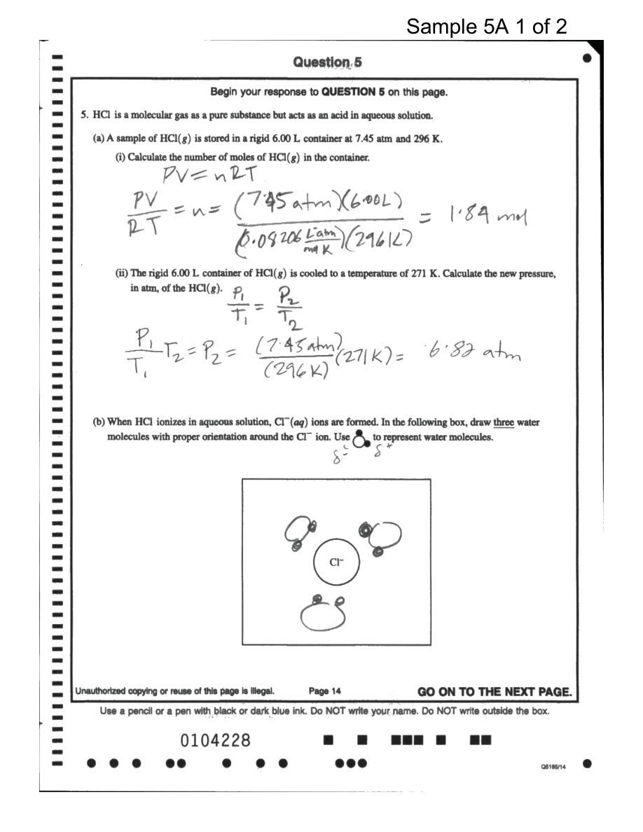
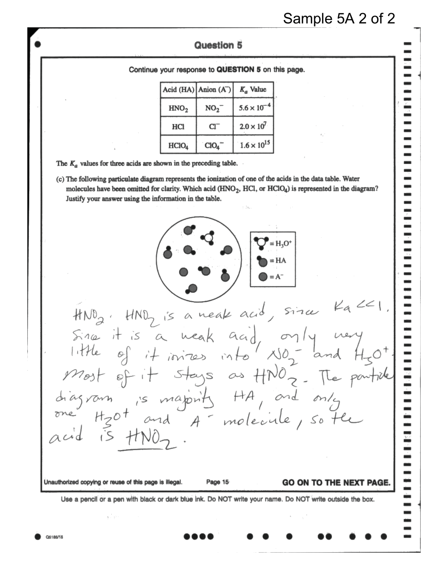
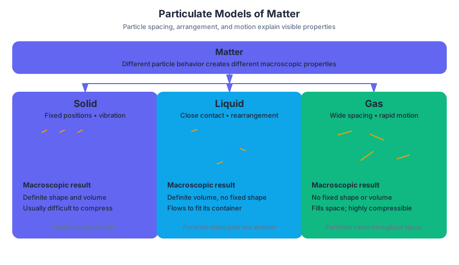
3.5 Kinetic Molecular Theory · 3.6 Deviation from Ideal Gas Law
Key concepts: Kinetic Molecular Theory (KMT) · Temperature as a macroscopic measure of the average kinetic energy of gas particles · Kinetic energy of moving particles · Particle models of gases · Maxwell–Boltzmann kinetic-energy distribution curves · Ideal-gas assumptions as a simplification · Deviation of real gases from ideal behavior · Interparticle attractions in real gases · Finite particle volume in real gases · Connections between particulate and macroscopic scales
A gas’s pressure and temperature are macroscopic clues to what its particles are doing at the microscopic scale: moving continuously, randomly, and with a range of kinetic energies.
3.5 Kinetic Molecular Theory · 3.6 Deviation from Ideal Gas Law
A gas’s pressure and temperature are macroscopic clues to what its particles are doing at the microscopic scale: moving continuously, randomly, and with a range of kinetic energies. Kinetic molecular theory (KMT) connects those invisible motions to measurable gas properties, while the behavior of real gases reveals where the ideal-gas model becomes too simple.
Kinetic Molecular Theory: motion behind gas behavior
KMT explains gas behavior by modeling particles as constantly moving and colliding. The particles in a sample do not all move at one identical speed; instead, their kinetic energies are distributed across a range.
3.5.A.1: The kinetic molecular theory (KMT) relates the macroscopic properties of gases to motions of the particles in the gas. The Maxwell–Boltzmann distribution describes the distribution of the kinetic energies of particles at a given temperature.
The kinetic energy of a moving particle is represented by
$$ KE=\frac{1}{2}mv^2 $$
where $m$ is the particle’s mass and $v$ is its speed. Because speed is squared, a faster particle has disproportionately more kinetic energy. Temperature is therefore not the kinetic energy of one particular molecule; it is a macroscopic measure related to the average kinetic energy of the particles in the sample.
Heating a gas increases its average kinetic energy. The particles move faster on average, and collisions with the container walls become more energetic. In a rigid container, this produces a greater pressure. Importantly, heating does not make every particle move at the same speed.
Maxwell–Boltzmann distributions
A Maxwell–Boltzmann distribution is a graph showing how many particles have each range of kinetic energies. The horizontal axis represents kinetic energy, and the vertical axis represents the number or fraction of particles possessing that energy.
When temperature increases, the distribution broadens and spreads toward higher kinetic energies. Its peak becomes lower because the particles are distributed across a wider range, while the average kinetic energy increases.
| Temperature change | Particle-level interpretation | Distribution change |
|---|---|---|
| Lower temperature | Particles move more slowly on average | Narrower curve concentrated at lower $KE$ |
| Higher temperature | Particles move faster on average, but still have varied speeds | Broader curve shifted toward higher $KE$ |
Worked example — heating a sealed aerosol can. Suppose a sealed, rigid can is warmed. The can’s volume and the amount of gas remain essentially constant. Heating broadens the kinetic-energy distribution and shifts more particles into higher-energy motion; those particles strike the walls more frequently and with greater momentum transfer. The macroscopic pressure inside the can rises, even though the particles themselves have not chemically changed.
The ideal-gas model and its limits
The ideal-gas model is a useful simplification. It treats gas particles as having negligible volume compared with the container and assumes that particles do not exert attractions on one another. It also represents their motion as continuous and random, with collisions modeled in a simplified way.
An ideal gas is not a claim that real particles have no size or attractions. It is a mathematical model that works best when those effects are too small to matter.
Real gases deviate from ideal behavior for two principal reasons identified in Essential Knowledge 3.6.A.1:
- Interparticle attractions become important when conditions approach condensation, especially at relatively low temperatures. Attractions pull particles toward one another, changing how freely they move and how strongly they collide with the container.
- Particle volume becomes important at extremely high pressures. Gas particles occupy real space, so the volume available for particle motion is smaller than the container volume assumed by the ideal model.
Worked example — compressing a gas near condensation. A sample of gas is cooled and compressed until it approaches condensation. Cooling lowers the particles’ average kinetic energy, so attractive forces have a greater opportunity to influence their motion. As pressure becomes very high, the particles’ finite volumes also become significant. An explanation at AP level must connect the observed non-ideal behavior to both the macroscopic conditions and these particulate causes.
Argumentation across scales
Topic 3.6 is tied to Science Practice 6: Argumentation, specifically 6.E: Provide reasoning to justify a claim using connections between particulate and macroscopic scales or levels. A strong response does not merely state that a gas “is non-ideal”; it identifies the condition—near condensation temperature or extremely high pressure—and explains the particle-level cause.
Named misconception — “All particles have the same kinetic energy at a given temperature.” Temperature describes an average, not a uniform value. The Maxwell–Boltzmann curve shows that particles have a distribution of kinetic energies; increasing temperature shifts the population toward higher energies while retaining a range of particle energies.
Retrieval check: A gas sample is heated, and its Maxwell–Boltzmann curve becomes broader and shifts toward higher kinetic energy. What microscopic change does this represent, and why can a real gas deviate from ideal behavior when compressed to extremely high pressure?
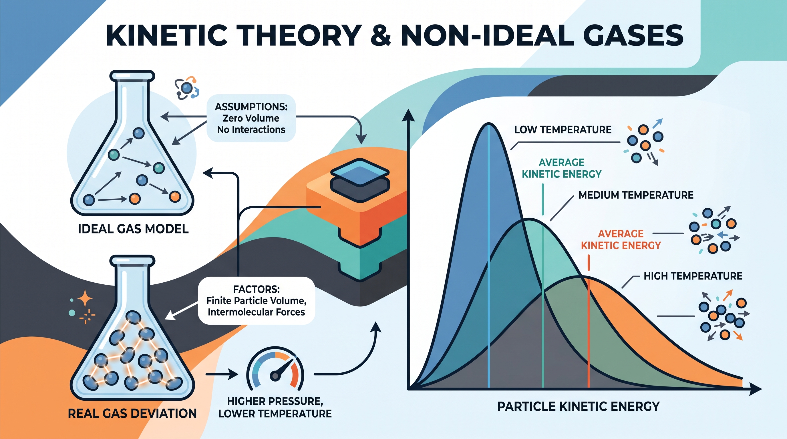
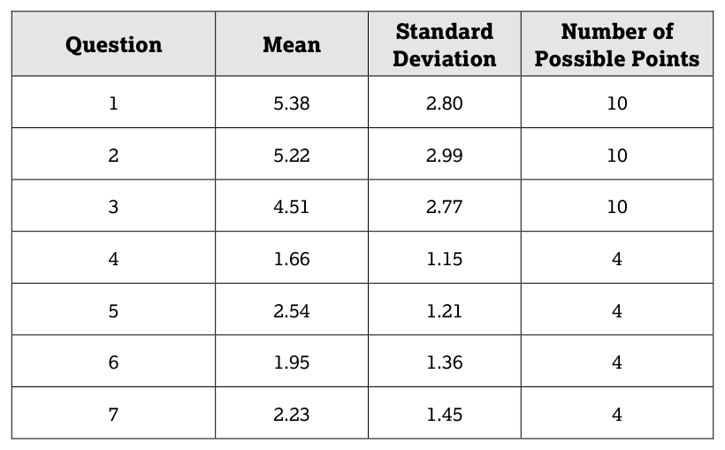
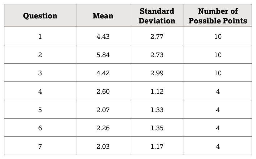
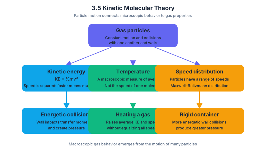
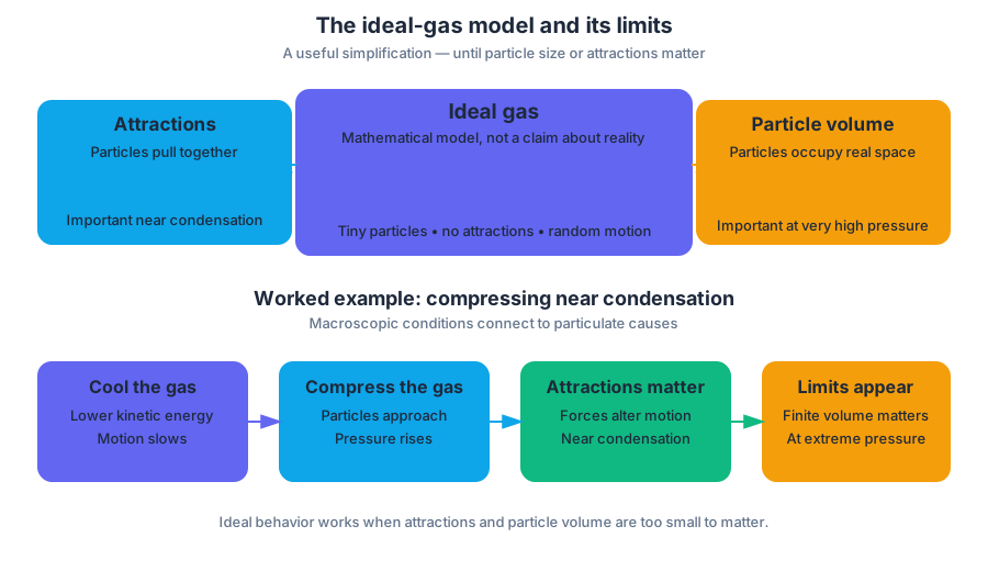
3.7 Solutions and Mixtures · 3.8 Representations of Solutions
Key concepts: Solutions · Mixtures · Representations of solutions · Learning objectives · Essential knowledge
A solution is a homogeneous mixture: its composition and macroscopic properties are uniform throughout the sample. A glass of saltwater looks uniform because the dissolved particles are distributed throughout the water, not because the salt has disappeared.
3.7 Solutions and Mixtures · 3.8 Representations of Solutions
A solution is a homogeneous mixture: its composition and macroscopic properties are uniform throughout the sample. A glass of saltwater looks uniform because the dissolved particles are distributed throughout the water, not because the salt has disappeared.
Solutions versus other mixtures
A mixture contains two or more substances physically combined. In a homogeneous mixture, the properties do not depend on where a sample is taken. In a heterogeneous mixture, properties can change from one location to another because the components are not uniformly distributed.
| Mixture type | Particle-level description | Macroscopic consequence |
|---|---|---|
| Homogeneous solution | Components are distributed uniformly at the scale being observed | A sample from any location has the same composition |
| Heterogeneous mixture | Components are unevenly distributed or remain in visibly distinct regions | Properties depend on location |
Solutions can exist as solids, liquids, or gases. Brass is a solid solution of metals, saltwater is a liquid solution, and air is a gaseous solution. The terms solute and solvent identify roles: the solute is the component dispersed in the solution, while the solvent is the component that dissolves it and is usually present in the larger amount.
Quantifying solution composition
The composition of a solution can be represented in several ways, but molarity is especially common in laboratory chemistry. Molarity, written $M$, is the amount of solute in moles per liter of solution:
$$ M=\frac{n_{\text{solute}}}{L_{\text{solution}}} $$
The denominator is the volume of the entire solution, not merely the volume of solvent. Rearranging the relationship lets you calculate any one of the three quantities:
$$ n_{\text{solute}}=M L_{\text{solution}} $$
$$ L_{\text{solution}}=\frac{n_{\text{solute}}}{M} $$
Worked example. A laboratory sample contains $0.250\ \mathrm{mol}$ of dissolved glucose in $0.500\ \mathrm{L}$ of solution. Its molarity is
$$ M=\frac{0.250\ \mathrm{mol}}{0.500\ \mathrm{L}} =0.500\ \mathrm{mol,L^{-1}} =0.500\ M $$
If the same solution were diluted until its total volume became $1.00\ \mathrm{L}$, the amount of glucose would remain $0.250\ \mathrm{mol}$, but the molarity would become
$$ M=\frac{0.250\ \mathrm{mol}}{1.00\ \mathrm{L}} =0.250\ M $$
The particles have not vanished; they are spread through a larger volume.
Key distinction: Molarity describes the ratio of solute amount to total solution volume. It is not the mass of solute, the volume of solvent, or the number of visible particles.
Topic 3.7: Solutions and Mixtures
Learning Objective 3.7.A: Calculate the number of solute particles, volume, or molarity of solutions.
Essential Knowledge 3.7.A.1 identifies solutions as homogeneous mixtures that may be solids, liquids, or gases. Their macroscopic properties do not vary throughout the sample, unlike those of a heterogeneous mixture, whose properties depend on location.
Essential Knowledge 3.7.A.2 states that solution composition can be expressed in several ways, with molarity being the most common representation in laboratory work. A reliable calculation begins by identifying the requested quantity, converting units when necessary, and applying the molarity relationship.
Topic 3.8: Representations of Solutions
Suggested Skill: Representing Data and Phenomena — 3.C: Represent visually the relationship between the structures and interactions across multiple levels or scales (e.g., particulate to macroscopic).
Learning Objective 3.8.A: Using particulate models for mixtures:
- i. Represent interactions between components.
- ii. Represent concentrations of components.
Essential Knowledge 3.8.A.1: Particulate representations of solutions communicate the structure and properties of solutions by showing the relative concentrations of the components and/or illustrating interactions among those components.
How to draw a strong particulate model
A useful model must do more than scatter dots randomly. It should connect the visible claim—such as “solution B is more concentrated”—to a particle-level cause: solution B contains more solute particles per equal volume of solution.
For example, two equal-volume beakers can represent a $0.20\ M$ and a $0.50\ M$ solution using identical solvent particles. The second beaker should show a greater number of solute particles in the same represented volume. If the solute is ionic, the model should show separated ions; if the solute remains molecular, it should show intact molecules.
Interactions also matter. In an aqueous ionic solution, water molecules orient their partially charged ends around ions: oxygen ends point toward cations, while hydrogen ends point toward anions. A particulate drawing that shows this arrangement explains why the ions are dispersed rather than displayed as an undissolved crystal.
Misconception check
Misconception: “A more concentrated solution must have more total particles.” Concentration compares solute amount with solution volume. A large volume of dilute solution may contain more total solute than a small volume of concentrated solution. Always compare the number of solute particles per equal volume.
Retrieval check
A model shows two equal-volume solutions. Beaker A contains twice as many solute particles as Beaker B, and both models show uniform distribution. Which is more concentrated, and what additional feature would the model need to explain an ion-containing solution?
Answer: Beaker A is more concentrated because it has more solute particles in the same volume. To explain an ionic solution, the model should show separated ions and the orientation of solvent particles around them, representing component interactions.
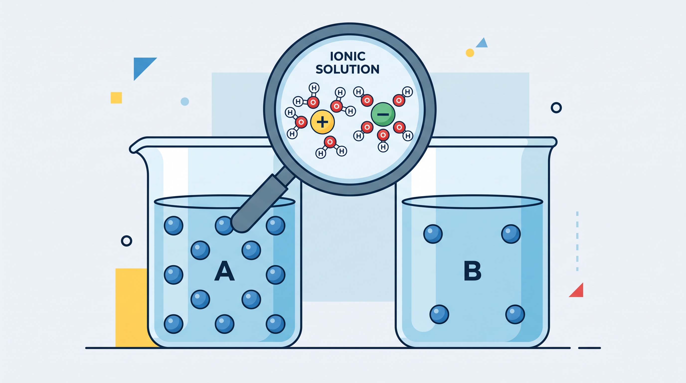
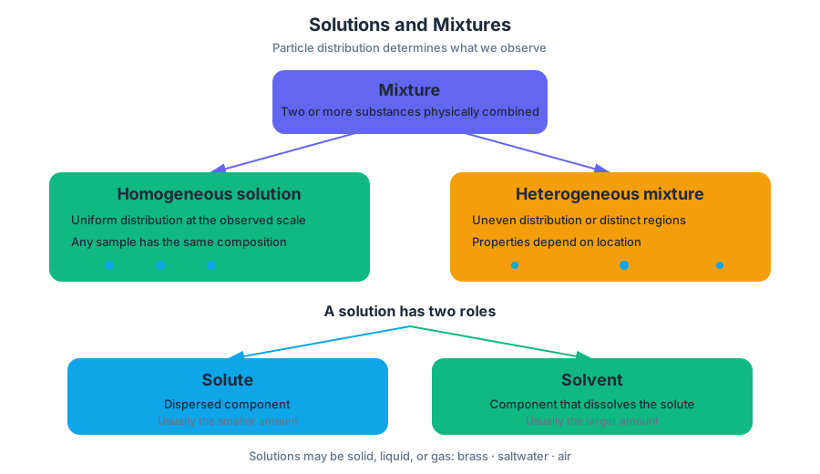
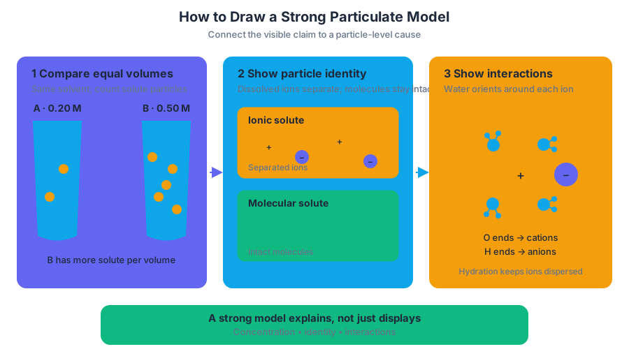
3.9 Separation of Solutions and Mixtures · 3.10 Solubility
Key concepts: Separation of solutions and mixtures · Chromatography · Chromatograms and relative polarity · Distillation · Differential intermolecular attractions · Solubility · Saturated solutions · Ion stoichiometry in dissolved compounds · Molar enthalpy of solution (ΔHsoln) · Temperature changes during dissolution
A dissolved substance cannot be removed from a true solution by ordinary filtration because its particles are distributed at the molecular or ionic scale. Separation becomes possible when a method exploits a difference in intermolecular attractions, volatility, or solubility.
3.9 Separation of Solutions and Mixtures · 3.10 Solubility
A dissolved substance cannot be removed from a true solution by ordinary filtration because its particles are distributed at the molecular or ionic scale. Separation becomes possible when a method exploits a difference in intermolecular attractions, volatility, or solubility.
Chromatography: separation by competing attractions
Chromatography separates components because each substance interacts differently with two phases: a mobile phase, which moves, and a stationary phase, which stays fixed. In paper, thin-layer, and column chromatography, a component that is more strongly attracted to the mobile phase travels farther; a component more strongly attracted to the stationary phase travels more slowly.
A chromatogram records the separated components as spots or bands. For a paper chromatogram, the relative distance traveled is often summarized by
$$ R_f=\frac{\text{distance traveled by solute}}{\text{distance traveled by solvent front}} $$
A larger $R_f$ means that the substance traveled farther under those conditions. If the stationary phase is relatively polar, a less-polar substance commonly spends more time in the mobile phase and has a larger $R_f$. This comparison is conditional: changing the solvent or stationary phase can change the order and distances.
CED alignment — Topic 3.9: Learning Objective 3.9.A, “Explain the results of a separation experiment based on intermolecular interactions,” rests on Essential Knowledge 3.9.A.1. The associated Suggested Skill is 2.C: Identify experimental procedures that are aligned to the question (which may include a sketch of a lab setup). This is Science Practice 2: Question and Method: choose chromatography when the question concerns different interactions with the two phases.
Worked interpretation
Suppose three dyes produce $R_f$ values of $0.18$, $0.52$, and $0.81$ on a polar paper strip. The dye with $R_f=0.18$ interacted most strongly with the paper relative to the solvent; the dye with $R_f=0.81$ interacted most strongly with the mobile phase. The chromatogram therefore supports a relative polarity interpretation, not an absolute polarity measurement.
Misconception check: “The largest spot must represent the most polar substance.” Spot size primarily reflects amount, concentration, and spreading. Travel distance—not spot area—is the evidence used for relative movement and interaction strength.
Distillation: separation by volatility
Distillation separates substances by taking advantage of differences in boiling point. A liquid with weaker intermolecular attractions escapes into the vapor phase more readily, giving it a higher vapor pressure and usually a lower boiling point. During distillation, the vapor becomes enriched in the more volatile component, then condensation collects that vapor as liquid.
Distillation is not the same as filtration. Filtration separates particles that differ greatly in physical size; distillation separates molecular species whose intermolecular attractions produce different vapor pressures. A mixture of liquids with very similar boiling points is difficult to separate completely because their vapor compositions remain similar.
Solubility and saturation
Solubility is the maximum amount of solute that dissolves in a specified quantity of solvent under specified conditions. A saturated solution contains dissolved solute at its solubility limit. Adding more solid to a saturated solution does not increase the dissolved concentration; the excess remains undissolved while dissolution and crystallization can occur dynamically.
For ionic compounds, the formula controls the ion ratio in solution. Dissolution of strontium hydroxide is represented by
$$ \mathrm{Sr(OH)_2(s)\rightleftharpoons Sr^{2+}(aq)+2OH^-(aq)} $$
Therefore,
$$ [\mathrm{OH^-}]=2[\mathrm{Sr^{2+}}] $$
If a saturated solution has $[\mathrm{Sr^{2+}}]=0.043\ \mathrm{M}$, then
$$ [\mathrm{OH^-}] =2(0.043\ \mathrm{M}) =0.086\ \mathrm{M} $$
The factor of $2$ is required by both atom conservation and charge balance: one $\mathrm{Sr^{2+}}$ requires two $\mathrm{OH^-}$ ions to produce electrically neutral dissolved formula units.
Misconception check: The concentration of hydroxide is not automatically equal to the concentration of strontium ions. Subscripts in the dissolution equation become stoichiometric concentration relationships.
Enthalpy of solution and temperature change
The molar enthalpy of solution, $\Delta H_{\mathrm{soln}}$, is the enthalpy change when one mole of an ionic compound dissolves in water. The observed temperature change depends on both this molar quantity and how much material dissolves:
$$ q=n\Delta H_{\mathrm{soln}} $$
For the surrounding solution, the same energy appears with the opposite sign:
$$ q_{\mathrm{solution}}=mc\Delta T $$
Thus, the magnitude of $\Delta T$ increases when more moles dissolve, when $|\Delta H_{\mathrm{soln}}|$ is larger, or when the solution has a smaller total heat capacity.
If equal masses of KCl and RbCl dissolve and the magnitude of their molar enthalpies of solution is approximately equal, their temperature changes are approximately equal when the solutions have equal specific heat capacities. The comparison must account for the number of moles, not merely the grams:
$$ n=\frac{m}{M} $$
Equal masses of substances with different molar masses contain different numbers of moles.
Retrieval check
A solution contains $0.020\ \mathrm{M}$ $\mathrm{Sr^{2+}}$ from saturated $\mathrm{Sr(OH)_2}$. Predict $[\mathrm{OH^-}]$ and identify whether chromatography or distillation would better separate two dissolved dyes with different attractions to polar paper.
Answer: $[\mathrm{OH^-}]=0.040\ \mathrm{M}$. Chromatography is appropriate because the dyes differ in their relative attractions to the mobile and stationary phases.
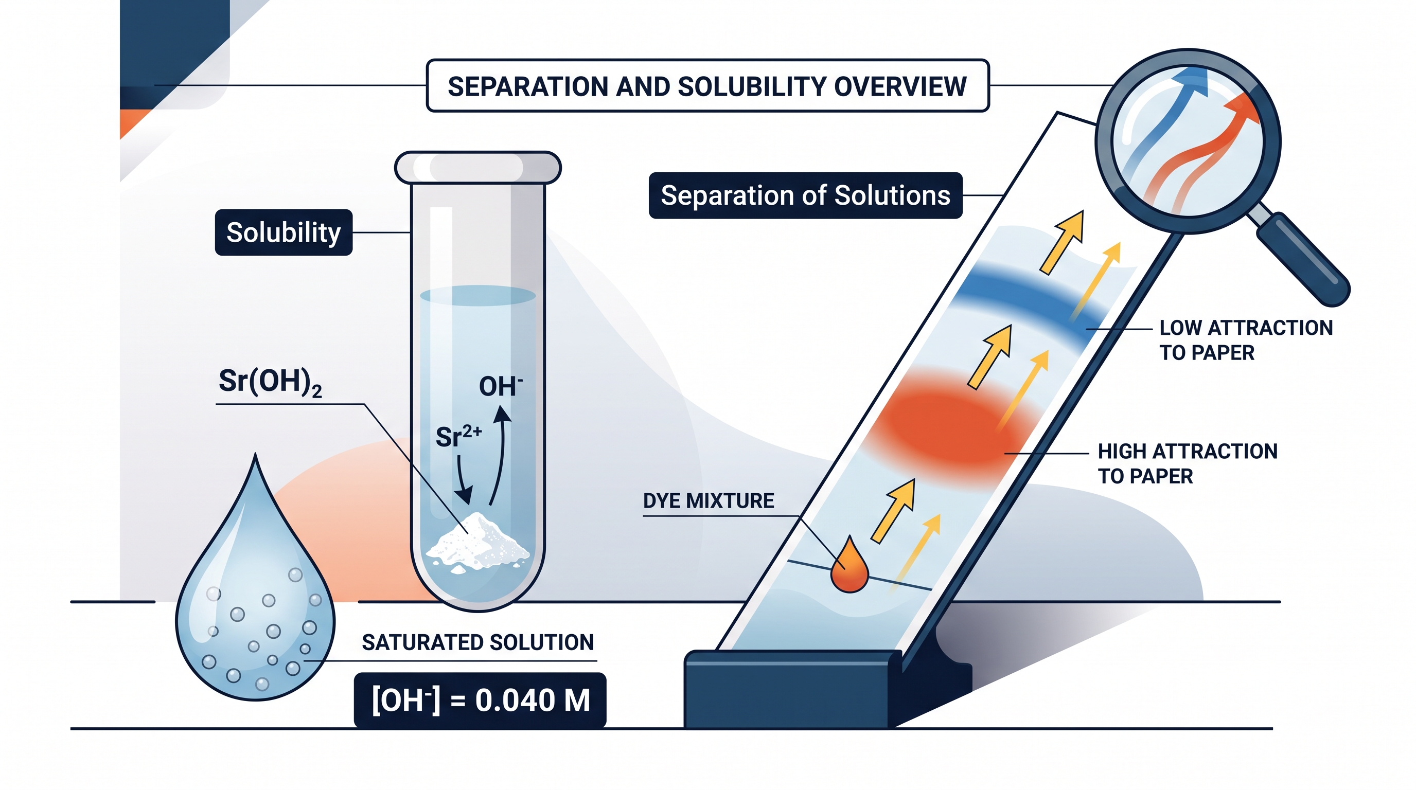
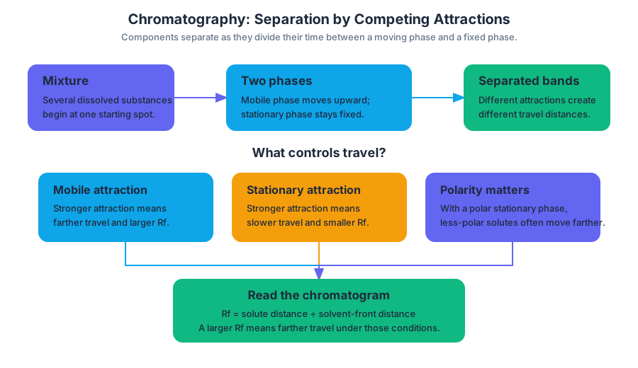
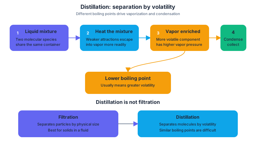
3.11 Spectroscopy and the Electromagnetic Spectrum · 3.12 Properties of Photons
Key concepts: Spectroscopy and the electromagnetic spectrum · Photons and their properties · Molecular motion associated with different spectral regions · Electronic transitions in atoms or molecules · Energy changes during electronic transitions · Relationship between photon energy and an electronic transition · Using models to explain atomic or molecular phenomena · Calculating an unknown quantity from known quantities using mathematical routines
A molecule can rotate, vibrate, or rearrange its electrons only by changing its energy. Spectroscopy studies how matter absorbs or emits electromagnetic radiation to reveal those energy changes.
3.11 Spectroscopy and the Electromagnetic Spectrum · 3.12 Properties of Photons
A molecule can rotate, vibrate, or rearrange its electrons only by changing its energy. Spectroscopy studies how matter absorbs or emits electromagnetic radiation to reveal those energy changes. The sharp question is: Why does microwave radiation make a molecule rotate, while ultraviolet radiation can move an electron to a different energy level?
Learning Objective 3.11.A: Explain the relationship between a region of the electromagnetic spectrum and the types of molecular or electronic transitions associated with that region.
The electromagnetic spectrum is the continuous range of electromagnetic radiation, organized by wavelength, frequency, and energy. A spectral region is a portion of that range whose photons have similar energies and therefore interact with matter in characteristic ways.
The key relationship is:
$$ c = \lambda \nu $$
where $c$ is the speed of light, $\lambda$ is wavelength, and $\nu$ is frequency. Because the speed of light is constant in a vacuum, wavelength and frequency are inversely related: shorter-wavelength radiation has higher frequency.
Different spectral regions correspond to different internal motions because the energy gaps between those motions differ.
| Spectral region | Matter’s response | Transition described |
|---|---|---|
| Microwave | Molecule changes its rotational state | Molecular rotational levels |
| Infrared | Bonds change their vibrational state | Molecular vibrational levels |
| Ultraviolet/visible | Electrons change energy levels | Electronic energy levels |
Photons: energy delivered in discrete packets
A photon is a discrete packet, or quantum, of electromagnetic energy. Matter does not absorb an arbitrary amount of light; an atom or molecule absorbs a photon when the photon’s energy exactly matches an allowed energy difference.
Essential Knowledge 3.11.A.1: Differences in absorption or emission of photons in different spectral regions are related to different types of molecular motion or electronic transition.
For a transition between two energy states,
$$ \Delta E_{\text{matter}} = E_{\text{photon}} $$
The sign depends on the process. During absorption, matter gains energy, so $\Delta E_{\text{matter}} > 0$. During emission, matter loses energy and releases a photon.
Photon energy is related to frequency by
$$ E = h\nu $$
and to wavelength by
$$ E = \frac{hc}{\lambda} $$
where $h$ is Planck’s constant, $6.626 \times 10^{-34}\ \mathrm{J \cdot s}$, and $c$ is approximately $3.00 \times 10^8\ \mathrm{m \cdot s^{-1}}$.
These equations produce two exam-ready conclusions:
- Higher-frequency photons have greater energy.
- Shorter-wavelength photons have greater energy.
A common misconception is that higher frequency means longer wavelength because both describe “more intense” light. Frequency and wavelength are not directly proportional: when $\nu$ increases, $\lambda$ decreases because $c = \lambda \nu$.
Worked example: calculating a photon’s energy
A photon has wavelength $500\ \mathrm{nm}$. Calculate its energy in joules.
First convert nanometers to meters:
$$ 500\ \mathrm{nm} \left(\frac{1\ \mathrm{m}}{10^9\ \mathrm{nm}}\right) = 5.00 \times 10^{-7}\ \mathrm{m} $$
Then substitute into the wavelength equation:
$$ E = \frac{(6.626 \times 10^{-34}\ \mathrm{J \cdot s})(3.00 \times 10^8\ \mathrm{m \cdot s^{-1}})} {5.00 \times 10^{-7}\ \mathrm{m}} $$
$$ E = 3.98 \times 10^{-19}\ \mathrm{J\ photon^{-1}} $$
The units demonstrate why dimensional analysis matters: meters cancel, seconds cancel, and the result is joules per photon. Because the wavelength has three significant figures, the final answer should be reported as $3.98 \times 10^{-19}\ \mathrm{J\ photon^{-1}}$.
Connecting spectra to molecular behavior
Microwave absorption changes a molecule’s rotational level. Infrared absorption changes the vibrational motion of bonds—such as stretching or bending. Ultraviolet or visible absorption changes an electron’s energy, often moving it from a lower-energy orbital or electronic state to a higher-energy state.
When an excited electron returns to a lower allowed energy level, the atom or molecule emits a photon. The emitted photon’s energy equals the energy difference between the two states:
$$ E_{\text{photon}} = E_{\text{higher}} - E_{\text{lower}} $$
A larger energy gap produces a higher-frequency, shorter-wavelength photon. This is why electronic transitions generally involve ultraviolet or visible radiation, while rotational and vibrational transitions involve lower-energy regions.
Misconception check: absorption does not mean that a molecule is destroyed or ionized automatically. It means that the molecule takes in a photon whose energy matches an allowed transition. Ionization occurs only if the absorbed energy is sufficient to remove an electron completely.
AP skills in action
This topic explicitly develops Science Practice 4, Model Analysis, especially 4.A: Predict and/or explain chemical properties or phenomena using given chemical theories, models, and representations. A spectrum, energy-level diagram, or molecular-motion model can be used to predict which type of transition occurred.
It also develops Science Practice 5, Mathematical Routines, specifically 5.F: Calculate, estimate, or predict an unknown quantity from known quantities by selecting and following a logical computational pathway and attending to precision. A strong solution identifies the known quantity, converts units before substitution, chooses $E=h\nu$ or $E=hc/\lambda$, and reports an appropriately precise result.
Retrieval check: A molecule absorbs infrared radiation and later emits a photon with a shorter wavelength than the absorbed photon. Is the emitted photon more energetic or less energetic? The shorter wavelength means higher frequency and therefore greater photon energy; the molecule’s emitted transition has the larger energy difference.
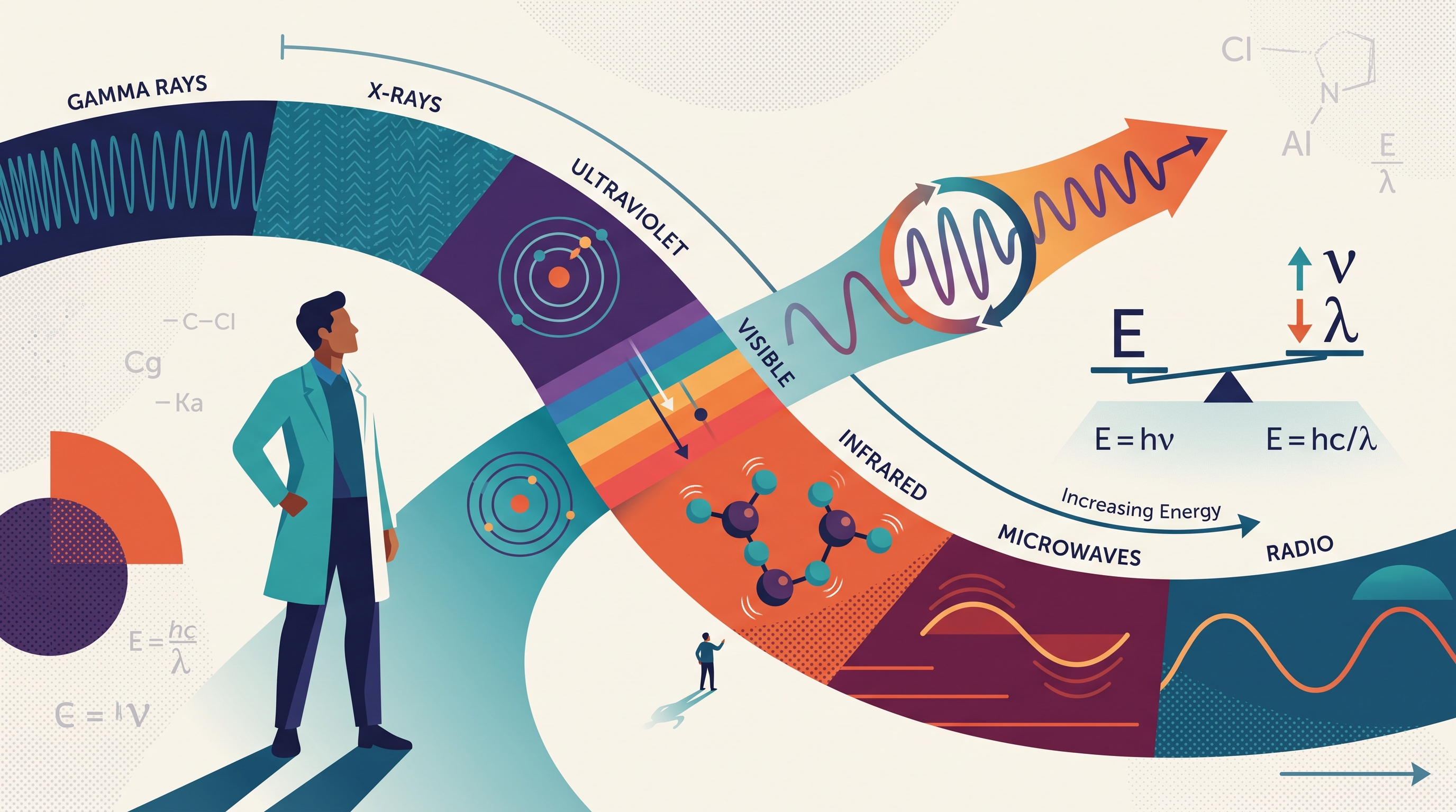
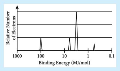
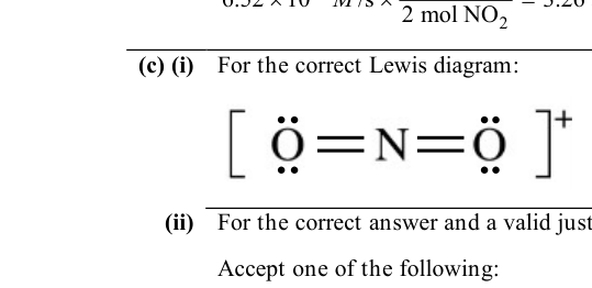
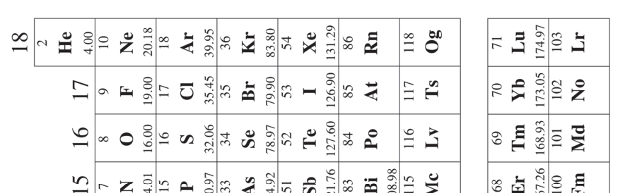
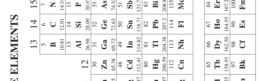
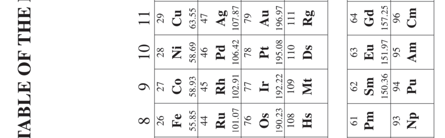
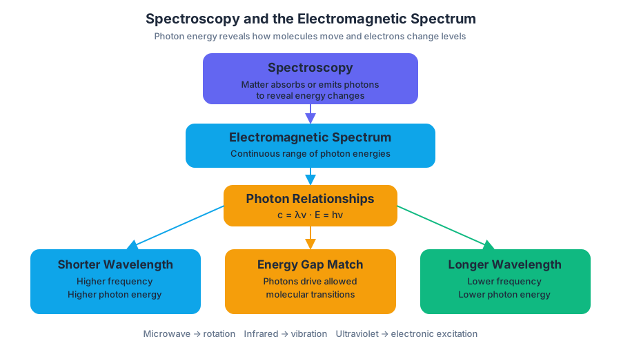
3.13 Beer-Lambert Law
Key concepts: Beer-Lambert Law · Linear relationship between absorbance and concentration · Effect of concentration on light absorption · Effect of path length on light absorption · Molar absorptivity · Calibration curves · Dilution calculations · Determining concentration from absorbance · Experimental error in absorbance measurements · V²⁺(aq) solution analysis
A solution looks transparent because some light passes through it—but even a faintly colored solution removes a measurable fraction of the light beam. The Beer-Lambert law connects that absorbed light to the number of absorbing particles in the beam, the distance the light travels through the solution, and the…
3.13 Beer-Lambert Law
A solution looks transparent because some light passes through it—but even a faintly colored solution removes a measurable fraction of the light beam. The Beer-Lambert law connects that absorbed light to the number of absorbing particles in the beam, the distance the light travels through the solution, and the species’ ability to absorb a particular wavelength.
Learning Objective 3.13.A: Explain the amount of light absorbed by a solution of molecules or ions in relationship to the concentration, path length, and molar absorptivity.
The central relationship
Absorbance, $A$, is a unitless measure of how strongly a solution reduces the intensity of transmitted light. The Beer-Lambert law is
$$ A=\varepsilon bc $$
where:
| Symbol | Meaning | Typical units |
|---|---|---|
| $A$ | Absorbance | Unitless |
| $\varepsilon$ | Molar absorptivity, the intensity with which a species absorbs light at a particular wavelength | $\mathrm{L,mol^{-1},cm^{-1}}$ |
| $b$ | Path length, or distance traveled by light through the solution | $\mathrm{cm}$ |
| $c$ | Concentration of the absorbing species | $\mathrm{mol,L^{-1}}$ |
The law says that absorbance increases directly with both concentration and path length when $\varepsilon$ and the wavelength remain constant. A solution with twice as many absorbing particles in the light path absorbs twice as much light; a cuvette twice as wide in the direction of the beam also produces twice the absorbance.
Why concentration and path length matter
Imagine shining a flashlight through a hallway containing colored balloons. Adding more balloons increases the chance that light encounters one. Keeping the same number of balloons but making the hallway longer also increases the number of balloons along the beam’s route. In a solution, the “balloons” are absorbing molecules or ions.
The molar absorptivity, $\varepsilon$, distinguishes substances and wavelengths. Two solutions with the same concentration and path length can have different absorbances because one chemical species may absorb that wavelength much more intensely than the other. Therefore, comparisons require the same wavelength and a known or constant path length.
Essential Knowledge 3.13.A.1: The Beer-Lambert law relates light absorption to molar absorptivity, path length, and concentration: $A=\varepsilon bc$. The path length, $b$, and concentration, $c$, are proportional to the number of light-absorbing particles in the light path.
Calibration curves: turning absorbance into concentration
A calibration curve is a graph of absorbance versus concentration for solutions whose concentrations are known. Under conditions where the Beer-Lambert law applies, the graph is linear:
$$ A=(\varepsilon b)c $$
Thus, the slope of a graph of $A$ versus $c$ is $\varepsilon b$, and an unknown concentration can be found by measuring its absorbance and locating the matching concentration on the line.
For example, suppose four equal amounts of absorbing ions produce an absorbance of $0.08$. The response is therefore $0.02$ absorbance per ion, or per corresponding concentration unit:
$$ \frac{0.08}{4}=0.020 $$
If an unknown solution gives $A=0.22$, then
$$ \text{concentration}=\frac{0.22}{0.020}=11 $$
in those calibration concentration units.
Worked laboratory example: $V^{2+}(aq)$
A calibration curve for $V^{2+}(aq)$ has slope $0.020\ \mathrm{L,mmol^{-1}}$ when measured in a $1.00\ \mathrm{cm}$ cuvette. A diluted vanadium solution has absorbance $0.22$.
Using $A=mc$, where $m$ is the calibration-curve slope,
$$ c_{\text{diluted}} =\frac{A}{m} =\frac{0.22}{0.020\ \mathrm{L,mmol^{-1}}} =11\ \mathrm{mmol,L^{-1}} $$
Therefore,
$$ c_{\text{diluted}}=0.011\ \mathrm{mol,L^{-1}} $$
If the sample was diluted by a factor of $10$, conservation of solute gives
$$ c_{\text{original}} =(10)(0.011\ \mathrm{mol,L^{-1}}) =0.11\ \mathrm{mol,L^{-1}} $$
The absorbance determines the concentration of the diluted sample first; the dilution factor must then be applied to recover the original molarity.
Misconception and experimental error
Misconception check: “A darker-looking solution always has a larger absorbance.” Not necessarily. Absorbance depends on wavelength, molar absorptivity, concentration, and path length. A pale solution measured at a strongly absorbed wavelength may have greater absorbance than a darker solution measured at a poorly absorbed wavelength.
For Suggested Skill 2.E — Question and Method: Identify or describe potential sources of experimental error, consider a dirty or scratched cuvette, fingerprints blocking the light path, bubbles, an incorrect blank, an inconsistent path length, or measuring at different wavelengths. These errors can shift the calibration curve or make individual absorbance measurements unreliable. A cuvette should be clean, oriented consistently, filled without bubbles, and compared with an appropriate blank.
Retrieval check: If concentration doubles while $\varepsilon$ and $b$ remain constant, what happens to $A$? If the path length is accidentally doubled, what happens to the calculated concentration when the original path length is incorrectly used? The first absorbance doubles; the second calculation overestimates concentration by a factor of $2$.

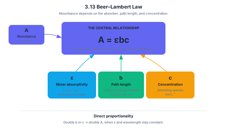
4.1 Introduction to Reactions · 4.2 Net Ionic Equations
Key concepts: Representing physical and chemical processes with chemical equations · Balanced molecular equations · Complete ionic equations · Net ionic equations · Conservation of mass in chemical reactions · Conservation of charge in chemical reactions · Writing equations for physical changes · Writing equations from the identities of reactants and products · Writing ionic equations for a given chemical reaction · Determining the limiting reactant and product yield
A chemical equation is a compact model of what happens when matter changes: it identifies the substances involved, shows how particles are rearranged, and records the numerical relationships required by conservation laws.
4.1 Introduction to Reactions · 4.2 Net Ionic Equations
A chemical equation is a compact model of what happens when matter changes: it identifies the substances involved, shows how particles are rearranged, and records the numerical relationships required by conservation laws. The central question is simple but powerful: How can symbols prove that atoms and charge are conserved while showing which particles actually react?
A physical change can also be written as an equation because the substance’s identity remains unchanged. For example, liquid water becoming vapor is represented as
$$ H_2O(l) \rightarrow H_2O(g) $$
The formula remains $H_2O$ on both sides; only the physical state changes. A chemical change, by contrast, rearranges atoms into new combinations, so at least one new chemical formula appears.
Conservation determines whether an equation is balanced
A balanced chemical equation has equal numbers of atoms of every element on both sides. This expresses conservation of mass: atoms are rearranged, not created or destroyed. For ionic reactions, the total charge must also be equal on both sides, expressing conservation of charge.
4.2.A.1: All physical and chemical processes can be represented symbolically by balanced equations.
4.2.A.2: Chemical equations represent chemical changes as rearrangements of atoms into new combinations. Equal numbers of atoms before and after demonstrate conservation of mass and charge.
Balance equations by changing coefficients, never subscripts. A coefficient changes the number of particles or formula units; changing a subscript changes the substance itself. For the reaction of hydrogen gas with oxygen gas:
$$ H_2(g) + O_2(g) \rightarrow H_2O(l) $$
There are two oxygen atoms on the left but only one on the right. Placing a coefficient of $2$ before water creates two oxygen atoms and four hydrogen atoms on the product side:
$$ 2H_2(g) + O_2(g) \rightarrow 2H_2O(l) $$
Now both elements are conserved.
Misconception check — “Balancing means making formulas symmetrical.” It does not. The formulas tell you which substances exist; coefficients tell you the reacting ratio. The equation above means $2$ molecules, formula units, or moles of $H_2$ react with $1$ of $O_2$ to form $2$ of $H_2O$.
Three symbolic views of one reaction
4.2.A.3 identifies three forms used according to context:
| Equation form | What it shows | Example purpose |
|---|---|---|
| Molecular equation | Compounds as intact formulas | Overall reaction and stoichiometric ratios |
| Complete ionic equation | Dissolved strong electrolytes separated into ions | Every aqueous particle present |
| Net ionic equation | Only species that chemically participate | The essential reaction |
Consider aqueous silver nitrate reacting with aqueous sodium chloride. The molecular equation is
$$ AgNO_3(aq) + NaCl(aq) \rightarrow AgCl(s) + NaNO_3(aq) $$
This balanced molecular equation represents the overall reaction. It shows that insoluble silver chloride forms, but it does not show that the aqueous compounds are present as ions.
In the complete ionic equation, soluble strong electrolytes are separated:
$$ Ag^+(aq) + NO_3^-(aq) + Na^+(aq) + Cl^-(aq) \rightarrow AgCl(s) + Na^+(aq) + NO_3^-(aq) $$
The ions $Na^+$ and $NO_3^-$ appear unchanged on both sides. They are spectator ions: present in solution but not chemically transformed.
Canceling the spectator ions gives the net ionic equation:
$$ Ag^+(aq) + Cl^-(aq) \rightarrow AgCl(s) $$
This equation shows the species that actually participate. It remains balanced in atoms and charge: one silver atom and one chlorine atom occur on each side, and the total charge is $+1-1=0$ on the left and $0$ for solid $AgCl$ on the right.
A reliable writing pipeline
When reactant or product identities are supplied, use this sequence:
- Write correct chemical formulas and physical states.
- Balance the molecular equation with coefficients.
- Separate only dissolved strong electrolytes in the complete ionic equation.
- Keep solids, liquids, gases, and weak electrolytes intact.
- Cancel identical spectator ions.
- Check atoms and total charge in the net ionic equation.
For example, calcium carbonate solid reacting with hydrochloric acid produces aqueous calcium ions, carbon dioxide gas, and liquid water:
$$ CaCO_3(s) + 2HCl(aq) \rightarrow CaCl_2(aq) + CO_2(g) + H_2O(l) $$
The complete ionic form is
$$ CaCO_3(s) + 2H^+(aq) + 2Cl^-(aq) \rightarrow Ca^{2+}(aq) + 2Cl^-(aq) + CO_2(g) + H_2O(l) $$
After canceling chloride ions:
$$ CaCO_3(s) + 2H^+(aq) \rightarrow Ca^{2+}(aq) + CO_2(g) + H_2O(l) $$
Misconception check — “Every aqueous substance splits.” Only soluble strong electrolytes are written as separate ions. A solid such as $AgCl(s)$ does not split in the equation, and a molecular substance such as $H_2O(l)$ remains intact.
AP reasoning practices in action
- Science Practice 1: Models and Representations — Select molecular, complete ionic, or net ionic notation to represent the relevant chemical scale.
- Science Practice 3: Representing Data and Phenomena — Translate an observed precipitate, gas formation, or phase change into a symbolic equation.
- Science Practice 4: Model Analysis — Test whether atoms, charge, phases, and spectator-ion cancellations are chemically consistent.
- Science Practice 5: Mathematical Routines — Use coefficients as mole ratios and balance equations systematically.
- Science Practice 6: Argumentation — Justify that a proposed equation is valid using conservation of atoms and charge.
Retrieval check: Write the net ionic equation for aqueous barium ions reacting with aqueous sulfate ions to form solid barium sulfate. Then verify both atom count and charge.
Answer:
$$ Ba^{2+}(aq) + SO_4^{2-}(aq) \rightarrow BaSO_4(s) $$
The atoms match, and the total charge is $0$ on both sides.
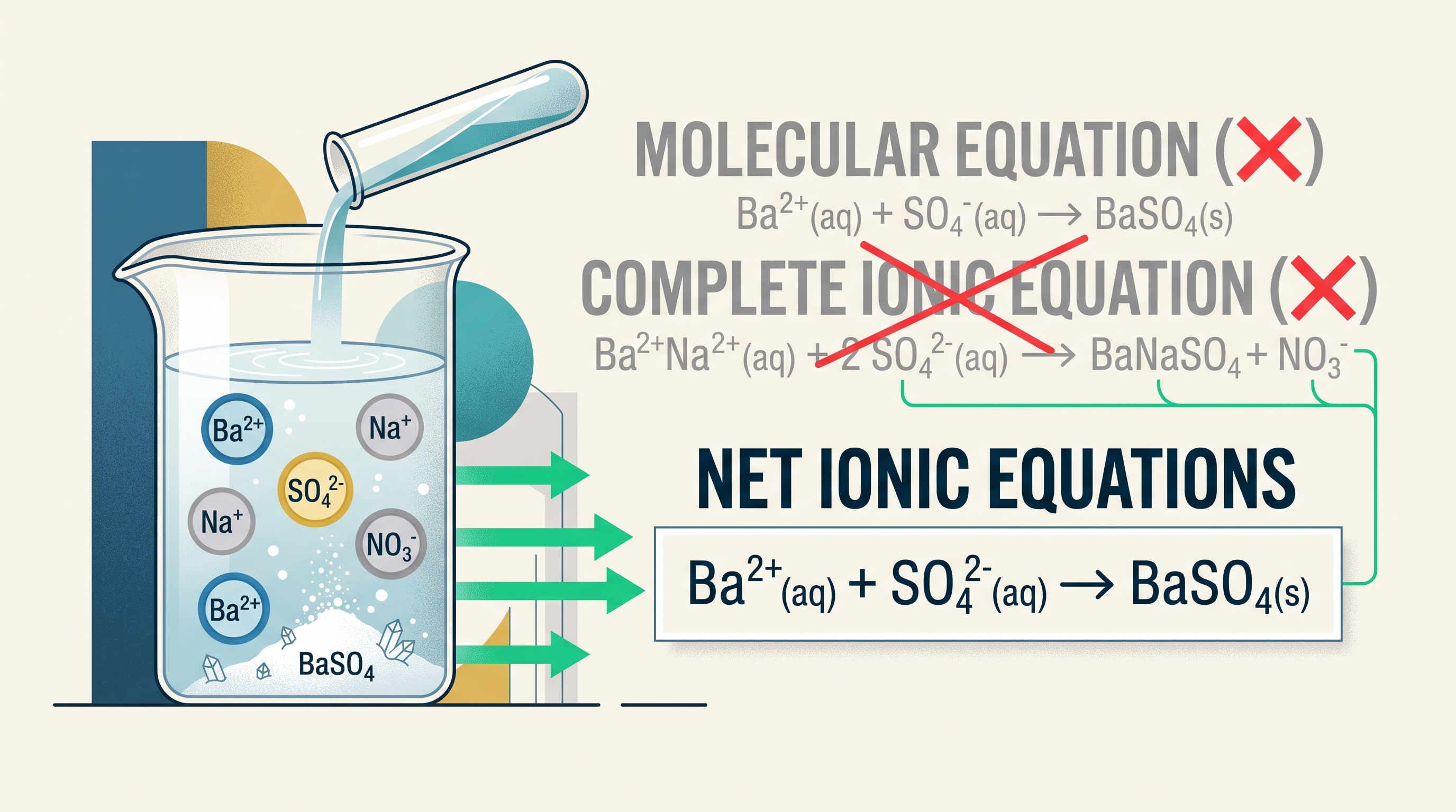
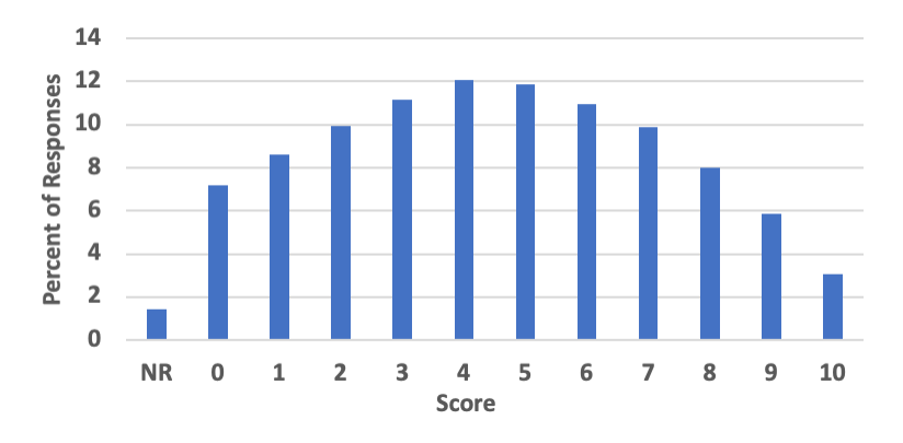
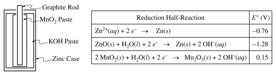
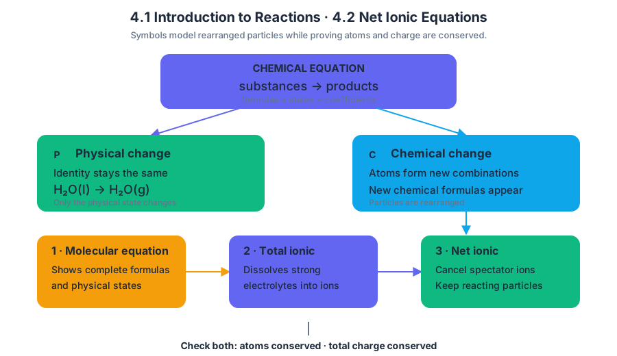
4.3 Representations of Reactions · 4.4 Physical and Chemical Changes
Key concepts: Representing chemical phenomena using data from laboratory setups or experimental results · Using evidence to explain changes and interactions of chemical substances · Distinguishing physical changes from chemical changes · Physical changes involve rearrangement of interactions without changing the substances · Melting as an example of a physical change · Formation and separation of mixtures as common physical changes · Chemical changes alter substances and produce different chemical species · Using representations of atoms or molecules to interpret chemical phenomena · Identifying potential sources of experimental error · Justifying claims about chemical phenomena with evidence and chemical principles
A substance can melt, mix, react, or separate while the visible result changes dramatically; the decisive question is whether the particles themselves remain the same.
4.3 Representations of Reactions · 4.4 Physical and Chemical Changes
A substance can melt, mix, react, or separate while the visible result changes dramatically; the decisive question is whether the particles themselves remain the same. Chemistry answers that question by connecting laboratory observations to particle-level representations and evidence.
Physical changes: new arrangement, same substances
Essential Knowledge 4.1.A.1: A physical change occurs when a substance undergoes a change in properties but not a change in composition.
During a physical change, the particles may move differently, spread farther apart, or rearrange their interactions, but the particles remain chemically identical. Melting is the classic example: solid water becomes liquid water, yet the particles are still $H_2O$ molecules.
A particle-level model of melting should show the same molecules before and after:
- Solid: $H_2O$ molecules occupy relatively fixed positions and vibrate in an organized arrangement.
- Liquid: the same $H_2O$ molecules remain present, but they move past one another and have less constrained arrangements.
- Conclusion: intermolecular attractions and particle arrangement change; chemical composition does not.
Formation and separation of mixtures are also common physical changes. Combining iron filings and sand produces a mixture containing iron and sand, not a new substance made from them. A magnet can then separate the iron because the original substances retain their identities. Similarly, evaporating water from a salt solution separates water from dissolved salt without requiring the salt particles to become a different chemical species.
Chemical changes: different chemical species
Essential Knowledge 4.1.A.2: A chemical change occurs when substances are transformed into new substances, typically with different compositions.
A chemical change rearranges atoms into new combinations. The atoms are not destroyed, but the original molecules or ions are transformed, so the products have different chemical identities and properties from the reactants.
Possible laboratory evidence includes production of heat or light, formation of a gas, formation of a precipitate, or a color change. These observations are clues, not automatic proof: a temperature change can result from physical dissolving, and a color change can arise from dilution or mixing. The strongest claim connects several observations to a particle-level explanation.
From laboratory evidence to a chemical claim
Use the following reasoning chain when interpreting an experimental setup or data table:
- Observation: State exactly what was measured or seen.
- Evidence: Identify the relevant change in temperature, color, gas production, precipitate formation, mass, or phase.
- Particle representation: Describe whether particles merely changed arrangement or were transformed into new species.
- Chemical principle: Use conservation of atoms and the distinction between composition and arrangement.
- Claim: Conclude whether the evidence supports a physical or chemical change.
Worked example — two samples in the laboratory. A student observes that ice melts in one beaker. In another, two clear solutions are mixed; the mixture becomes cloudy and a solid settles.
- For the ice, the observation is a phase change from solid to liquid. A particle model contains $H_2O$ molecules before and after, so the change is physical.
- For the mixed solutions, the observation is formation of a precipitate. If the solid contains a new combination of ions, the particle model shows new chemical species forming, so the evidence supports a chemical change.
- The conclusion is not based merely on “something visible happened.” It follows from comparing particle identities and composition.
Misconception check — “Any color change proves a reaction.” Not necessarily. A color may become lighter because a solution was diluted, which changes the arrangement and concentration of particles without creating a new substance. Color change becomes stronger evidence for chemical change when it occurs with other evidence, such as gas formation or precipitate formation, and when a particle-level explanation accounts for it.
Representations, data, and experimental error
Chemical phenomena can be represented at several levels: a laboratory photograph or data table shows the macroscopic level; particle diagrams show atoms, molecules, or ions; and chemical equations symbolize the transformation. A good representation preserves the important evidence rather than merely illustrating appearance.
Science Practice 2 — Question and Method, Skill 2.B: “Identify evidence of chemical and physical changes in matter.” A student applying this skill must formulate a hypothesis or predict results, then decide which observations would distinguish unchanged substances from newly formed species.
Science Practice 2 — Question and Method, Skill 2.E: “Identify or describe potential sources of experimental error.” Examples include a thermometer touching the container instead of the solution, incomplete mixing, contamination from a previous trial, an unreadable precipitate, or gas escaping before its amount is recorded. Each error should be tied to its likely effect on the evidence.
Science Practice 2 — Question and Method, Skill 2.F: “Explain how modifications to an experimental procedure will alter results.” For example, if a student removes a filter paper before all liquid has passed through, some solid may remain in the filtrate. The apparent separation is then incomplete—not because the substances changed identity, but because the procedure failed to isolate them fully.
Science Practice 3 — Create representations or models of chemical phenomena requires translating observations into a particle-level model. Science Practice 4 — Model Analysis asks whether that model actually explains the data. Science Practice 6 — Argumentation requires supporting the physical- or chemical-change claim with evidence and chemical principles rather than with an unsupported visual impression.
Retrieval check
Which events are definitely physical changes: ice melting and salt-solution evaporation? Explain why both preserve particle identity and composition. In ice melting, $H_2O$ molecules remain $H_2O$ molecules; only their motion and arrangement change. In salt-solution evaporation, water particles leave the mixture while salt particles remain chemically unchanged. Both therefore alter phase, arrangement, or mixture composition without transforming the substances into different chemical species.
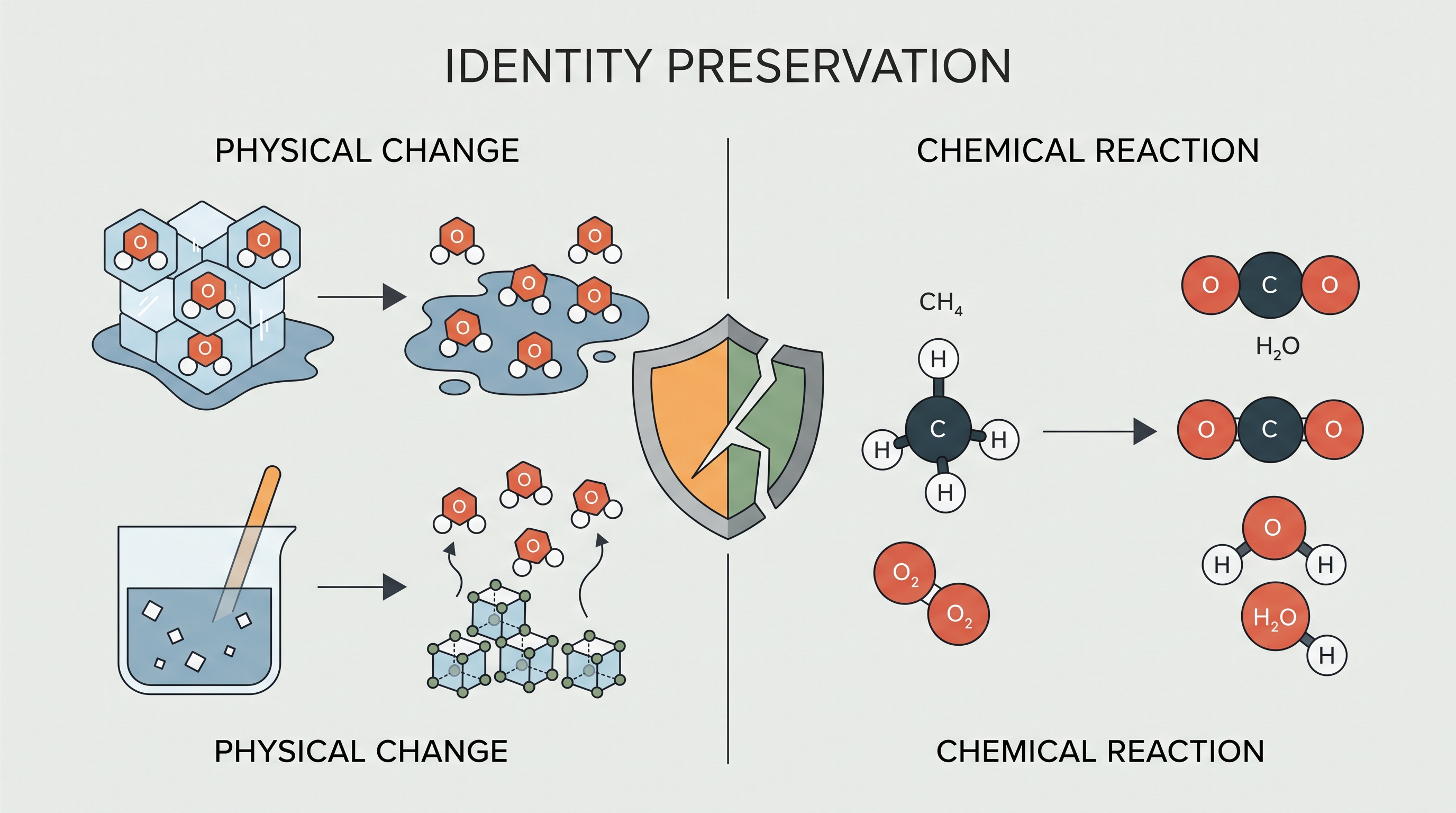
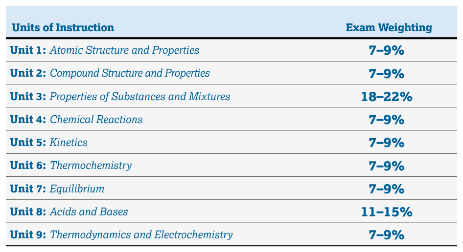

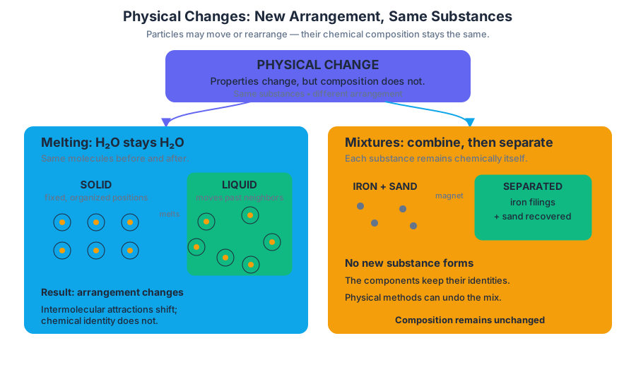
4.5 Stoichiometry · 4.6 Introduction to Titration
Key concepts: Advanced stoichiometry · Gas laws · The ideal gas law · Aqueous solution chemistry · Molarity · Introduction to titration · Practical laboratory applications · Investigation 7 · Purification applications
A chemical equation becomes experimentally useful only when its coefficients are treated as a quantitative recipe: they connect particles, moles, masses, gas volumes, and solution concentrations.
4.5 Stoichiometry · 4.6 Introduction to Titration
A chemical equation becomes experimentally useful only when its coefficients are treated as a quantitative recipe: they connect particles, moles, masses, gas volumes, and solution concentrations.
The stoichiometric map
A balanced equation such as
$$ 2H_2(g)+O_2(g)\rightarrow 2H_2O(g) $$
does not say that $2\ \mathrm{g}$ of hydrogen reacts with $1\ \mathrm{g}$ of oxygen. Its coefficients give mole relationships: $2$ mol $H_2$ react with $1$ mol $O_2$ to produce $2$ mol $H_2O$. Every advanced stoichiometry problem is a controlled conversion through that ratio.
The general pathway is:
$$ \text{given quantity} \rightarrow \text{moles of given substance} \rightarrow \text{moles of desired substance} \rightarrow \text{requested unit} $$
The middle conversion uses the coefficients of the balanced equation. The first and last conversions depend on the form of the data: molar mass for mass, $PV=nRT$ for gases, and molarity for aqueous solutions.
Gas stoichiometry: using $PV=nRT$
For a gas, the ideal gas law relates pressure, volume, amount, and temperature:
$$ PV=nRT $$
Here, $P$ is pressure, $V$ is volume, $n$ is amount in moles, $R$ is the gas constant, and $T$ is absolute temperature in kelvins. The temperature must be converted using $T(\mathrm{K})=T(^\circ\mathrm{C})+273.15$.
Worked example: identifying the limiting reactant
A reaction produces hydrogen gas according to
$$ Mg(s)+2HCl(aq)\rightarrow MgCl_2(aq)+H_2(g) $$
Suppose $0.120$ mol of magnesium reacts with $0.180$ mol of hydrochloric acid. Magnesium would require
$$ 0.120\ \mathrm{mol\ Mg}\times \frac{2\ \mathrm{mol\ HCl}}{1\ \mathrm{mol\ Mg}} =0.240\ \mathrm{mol\ HCl} $$
Only $0.180$ mol $HCl$ is available, so $HCl$ is the limiting reactant. The amount of hydrogen is therefore
$$ 0.180\ \mathrm{mol\ HCl}\times \frac{1\ \mathrm{mol\ H_2}}{2\ \mathrm{mol\ HCl}} =0.0900\ \mathrm{mol\ H_2} $$
At $298\ \mathrm{K}$ and $1.00\ \mathrm{atm}$,
$$ V=\frac{nRT}{P} =\frac{(0.0900)(0.08206)(298)}{1.00} =2.20\ \mathrm{L} $$
The limiting reactant controls the product amount; the excess reactant does not.
Misconception check — “The reactant with fewer grams is limiting.” Limiting status cannot be judged from mass alone. Convert each reactant to the amount of product it could form, or compare the available-to-required mole ratios. A large mass of a substance with a large molar mass may represent fewer moles than expected.
Aqueous stoichiometry and molarity
Molarity is the amount of solute per liter of solution:
$$ M=\frac{n}{V} $$
where $M$ has units of $\mathrm{mol,L^{-1}}$ and $V$ must be measured in liters. Rearranging gives the especially useful relationship
$$ n=MV $$
Thus, a measured solution volume can enter a stoichiometric calculation directly after multiplication by its molarity.
For example, $25.00\ \mathrm{mL}$ of $0.1500\ \mathrm{M}$ $NaOH$ contains
$$ n=(0.1500\ \mathrm{mol,L^{-1}})(0.02500\ \mathrm{L}) =0.003750\ \mathrm{mol\ NaOH} $$
If the reaction requires a $1:1$ mole ratio between $NaOH$ and another reactant, then $0.003750$ mol of that reactant is consumed. If the ratio is not $1:1$, the balanced equation—not the volumes alone—determines the conversion.
CED traceability: Topic 4.5 Stoichiometry centers on Learning Objective 4.5.A and includes the quantitative integration identified in Essential Knowledge 4.5.A.3: stoichiometric reasoning may involve masses, gas quantities, and molarity in aqueous solutions.
Titration: measuring an unknown concentration
A titration determines an unknown concentration by reacting the unknown solution with a solution of known concentration. The known solution is the titrant; the solution being analyzed is the sample. A buret delivers the titrant while the volume required for the reaction is measured accurately.
At the reaction’s equivalence point, stoichiometrically sufficient titrant has been added. An indicator may produce a visible color change near this point, but the indicator’s color change is an experimental signal, not the definition of equivalence.
For a $1:1$ reaction, the calculation is often
$$ M_{\text{unknown}}V_{\text{unknown}}
M_{\text{titrant}}V_{\text{titrant}} $$
For any other ratio, first calculate titrant moles and then apply the balanced-equation mole ratio.
Titration example
If $18.60\ \mathrm{mL}$ of $0.1000\ \mathrm{M}$ $NaOH$ neutralizes $25.00\ \mathrm{mL}$ of a monoprotic acid $HA$,
$$ n_{NaOH}=(0.1000)(0.01860)=0.001860\ \mathrm{mol} $$
Because
$$ HA+NaOH\rightarrow NaA+H_2O $$
has a $1:1$ ratio,
$$ M_{HA}=\frac{0.001860}{0.02500} =0.07440\ \mathrm{M} $$
Misconception check — “Equivalence point means equal volumes.” Equal volumes matter only in special cases. Equivalence means equal stoichiometric amounts after accounting for the reaction coefficients. A $2:1$ reaction requires a different relationship between the measured volumes and concentrations.
Investigation 7: from measurement to purification
Investigation 7 provides a practical setting for connecting mathematical chemistry to a laboratory process such as determining composition, monitoring a reaction, or evaluating purification. A defensible investigation records initial and final buret readings, solution concentrations, sample volume, balanced-equation ratios, calculations, uncertainty, and a conclusion supported by measured evidence.
The laboratory sequence is:
- Measure the sample or product carefully.
- Add titrant until the endpoint is reached.
- Convert titrant volume to moles using $n=MV$.
- Use the balanced equation to determine moles of the unknown.
- Convert to concentration, mass, purity, or yield.
- Compare the result with a claimed or expected value.
This is where Science Practice 1: Models and Representations, especially 1.B, becomes visible: the balanced equation is a particulate-level model that predicts the macroscopic volume required in the buret. Science Practice 3: Representing Data and Phenomena supports recording and interpreting buret data; Science Practice 5: Mathematical Routines supports dimensional analysis and significant figures; and Science Practice 6: Argumentation supports a conclusion linking the calculated amount to evidence.
Retrieval check
A $0.250\ \mathrm{M}$ solution provides $0.00500\ \mathrm{mol}$ of titrant. If the balanced reaction requires $2$ mol of titrant per $1$ mol of analyte, the analyte amount is
$$ 0.00500\ \mathrm{mol}\times\frac{1\ \mathrm{mol\ analyte}}{2\ \mathrm{mol\ titrant}} =0.00250\ \mathrm{mol} $$
The essential question is not “What formula applies?” but “What measured quantity must be converted into moles, and what coefficient ratio connects it to the unknown?”
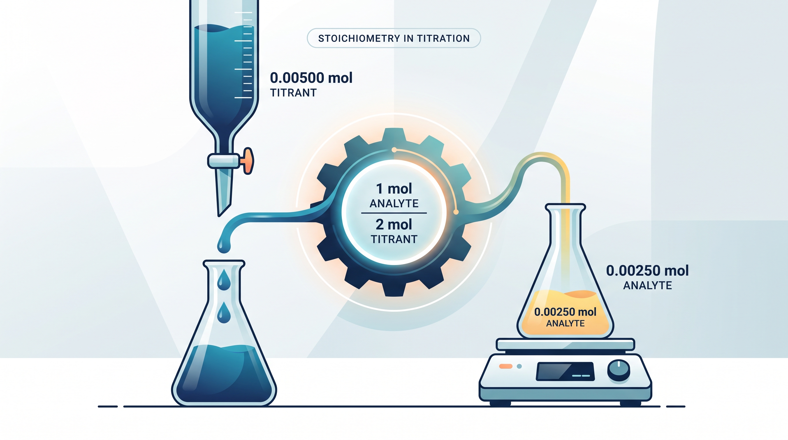
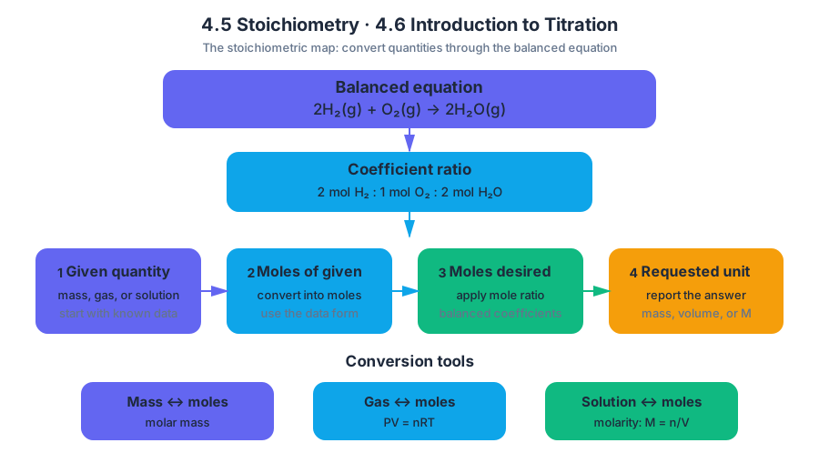
4.7 Types of Chemical Reactions · 4.8 Introduction to Acid-Base Reactions
Key concepts: Types of chemical reactions · Acid-base reactions · Oxidation-reduction reactions · Precipitation reactions · Identifying and representing chemical reactions · Balancing chemical equations · Solubility of salts in water · Justifying reaction classifications using chemical principles
A chemical equation is more than a recipe: it is a compact model of particles rearranging, electrons moving, or protons transferring. The central diagnostic question is: what changes between reactants and products?
4.7 Types of Chemical Reactions · 4.8 Introduction to Acid-Base Reactions
A chemical equation is more than a recipe: it is a compact model of particles rearranging, electrons moving, or protons transferring. The central diagnostic question is: what changes between reactants and products?
Learning Objective 4.7.A: Identify a reaction as acid-base, oxidation-reduction, or precipitation.
| Reaction type | What moves or forms? | Fastest chemical evidence |
|---|---|---|
| Acid-base | One or more protons, $H^+$ | A proton donor transfers $H^+$ to a proton acceptor |
| Oxidation-reduction | One or more electrons | Oxidation numbers change |
| Precipitation | An insoluble ionic solid | Aqueous ions combine to form a solid product |
Representing a reaction accurately
A chemical equation must conserve atoms and, for ionic equations, charge. A balanced equation therefore expresses the same number of atoms of each element on both sides; its coefficients describe particle or mole ratios, while subscripts belong to the chemical formula and must not be changed during balancing.
For example, magnesium burns in oxygen:
$$ 2Mg(s)+O_2(g)\rightarrow 2MgO(s) $$
The coefficient $2$ means that two magnesium atoms—or two moles of magnesium—react for every one oxygen molecule—or one mole of oxygen molecules. Changing $MgO$ to $Mg_2O$ would not balance the equation; it would invent a different substance.
Worked example — balancing by inspection. Start with propane combustion:
$$ C_3H_8+O_2\rightarrow CO_2+H_2O $$
Balance carbon first: $3CO_2$. Then balance hydrogen: $4H_2O$. The products contain $10$ oxygen atoms, so use $5O_2$:
$$ C_3H_8+5O_2\rightarrow 3CO_2+4H_2O $$
This is also a redox reaction because carbon and oxygen change oxidation numbers. Complete combustion of a hydrocarbon produces carbon dioxide and water, making combustion an important subclass of oxidation-reduction reactions.
Acid-base reactions: follow the proton
An acid-base reaction involves the transfer of one or more protons, $H^+$, between chemical species. In the Brønsted-Lowry model, an acid donates $H^+$ and a base accepts $H^+$.
A clear example is the reaction of ammonia with water:
NH_3(aq)+H_2O(l)\rightleftharpoons NH_4^+(aq)+OH^-(aq)
Water donates a proton to $NH_3$, so water acts as the acid. Ammonia accepts that proton, so it acts as the base. The paired species $H_2O/OH^-$ and $NH_4^+/NH_3$ are conjugate acid-base pairs: each pair differs by exactly one $H^+$.
A neutralization is a common acid-base pattern. For a strong acid and strong base, the net ionic equation is:
$$ H^+(aq)+OH^-(aq)\rightarrow H_2O(l) $$
Misconception check — “An acid-base reaction must have $H^+$ written as a reactant.” Not necessarily. Proton transfer may occur between molecular species, as in the ammonia example. Identify the donor and acceptor by comparing formulas before and after the reaction.
Precipitation reactions: inspect the ions
A precipitation reaction occurs when aqueous reactants produce an insoluble or sparingly soluble ionic compound. The new solid is written with the state symbol $(s)$; aqueous ions that remain dissolved are spectators and cancel from the net ionic equation.
Suppose aqueous silver nitrate is mixed with aqueous sodium chloride:
$$ AgNO_3(aq)+NaCl(aq)\rightarrow AgCl(s)+NaNO_3(aq) $$
The complete ionic equation is:
$$ Ag^+(aq)+NO_3^-(aq)+Na^+(aq)+Cl^-(aq)\rightarrow AgCl(s)+Na^+(aq)+NO_3^-(aq) $$
Canceling the unchanged spectator ions gives:
$$ Ag^+(aq)+Cl^-(aq)\rightarrow AgCl(s) $$
The required solubility knowledge is deliberately limited: all sodium, potassium, ammonium, and nitrate salts are soluble in water. Rote memorization of additional solubility rules is not assessed. The chemical principle matters more than a long memorized list: determine whether the possible ionic product is insoluble enough to leave solution as a solid.
Redox as a second diagnostic
An oxidation-reduction reaction, or redox reaction, transfers electrons between chemical species. Because electrons are rarely written directly in an ordinary molecular equation, identify redox by tracking oxidation numbers: oxidation is an increase in oxidation number, and reduction is a decrease.
For the reaction
magnesium changes from $0$ to $+2$, so it is oxidized. Oxygen changes from $0$ to $-2$, so it is reduced. The same reaction can belong to more than one category: combustion is redox, and some acid-base reactions can also involve oxidation-number changes.
Misconception check — “Any reaction with oxygen is automatically combustion.” Oxygen participation alone is not enough for the complete-combustion pattern. For hydrocarbons, complete combustion specifically produces $CO_2$ and $H_2O$; classification still requires examining the actual chemical change.
AP reasoning and retrieval check
The primary assessed science practice is Science Practice 1: Models and Representations, especially Skill 1.B: Describe the components of and quantitative information from models and representations that illustrate both particulate-level and macroscopic-level properties. Explain both what you observe—such as a solid forming—and what particles must be doing—such as ions leaving solution to form an ionic lattice.
Use Science Practice 6: Argumentation when justifying a classification: state the reaction type, cite the equation or observation as evidence, and connect that evidence to proton transfer, electron transfer, or solid formation. Use Science Practice 5: Mathematical Routines when balancing coefficients and verifying conservation of atoms and charge.
Retrieval check. Classify each reaction and give one chemical justification:
- $HCl(aq)+NH_3(aq)\rightarrow NH_4^+(aq)+Cl^-(aq)$
- $Ba^{2+}(aq)+SO_4^{2-}(aq)\rightarrow BaSO_4(s)$
- $Zn(s)+Cu^{2+}(aq)\rightarrow Zn^{2+}(aq)+Cu(s)$
Answers: (1) acid-base, because $NH_3$ accepts $H^+$; (2) precipitation, because an insoluble solid forms; (3) redox, because zinc is oxidized and copper ions are reduced. In every case, the justification identifies the chemical principle—not merely the reaction’s visual pattern.
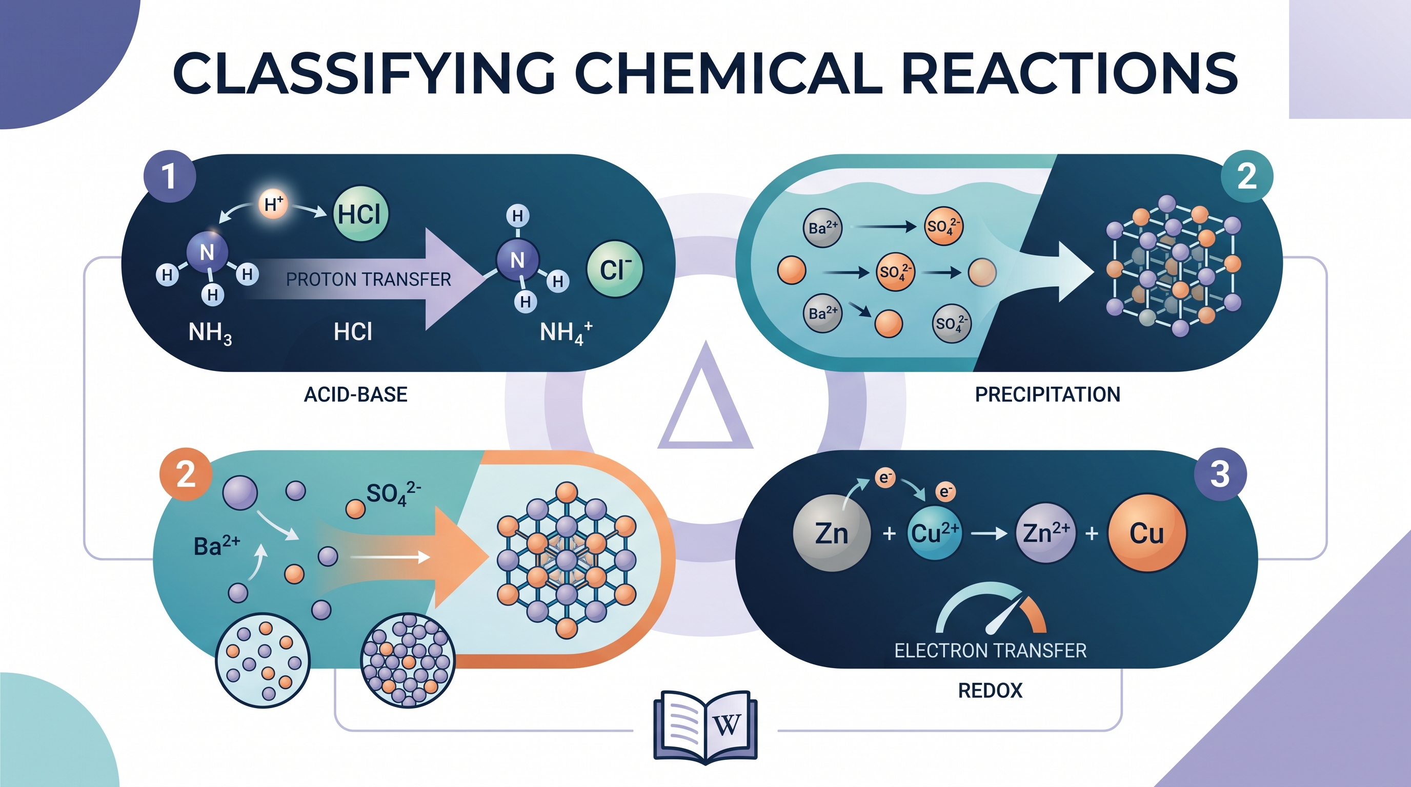
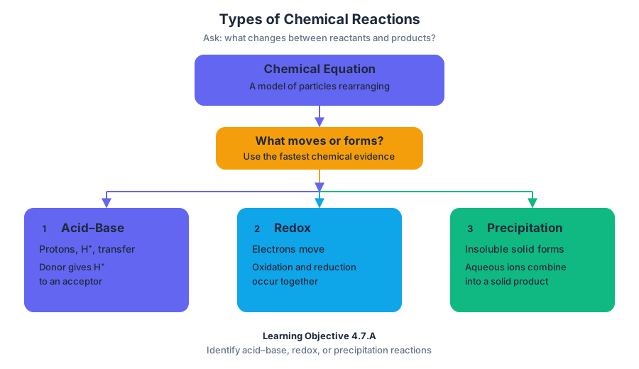
4.9 Oxidation-Reduction Reactions
Key concepts: Oxidation and reduction half-reactions · Electrochemical cells and thermodynamic favorability · Standard reduction and oxidation potentials · Calculating standard cell potential · Balancing redox equations and electron transfer · Anodes, cathodes, and galvanic cells · Gibbs free energy and electrochemical cells · Alkaline battery redox chemistry · Electroplating and oxidation of water · Rhodium plating of silver
Oxidation-reduction reactions, or redox reactions, transfer electrons from one chemical species to another: oxidation is electron loss, while reduction is electron gain. The memory aid LEO says GER captures the bookkeeping: Loss of Electrons is Oxidation; Gain of Electrons is Reduction.
4.9 Oxidation-Reduction Reactions
Oxidation-reduction reactions, or redox reactions, transfer electrons from one chemical species to another: oxidation is electron loss, while reduction is electron gain. The memory aid LEO says GER captures the bookkeeping: Loss of Electrons is Oxidation; Gain of Electrons is Reduction.
Oxidation: loss of electrons.
Reduction: gain of electrons.
A redox reaction can be separated into two half-reactions, equations that show the oxidation and reduction processes independently. For example, aluminum atoms lose three electrons:
$$ \mathrm{Al(s) \rightarrow Al^{3+}(aq) + 3e^-} $$
The electrons appear among the products because aluminum is oxidized. A reduction half-reaction places electrons among the reactants, such as:
$$ \mathrm{Au^{3+}(aq) + 3e^- \rightarrow Au(s)} $$
Electrochemical cells: where electron transfer becomes voltage
An electrochemical cell uses a redox reaction to move electrons through an external circuit or, in the reverse situation, uses an external power source to force electron transfer. The electrode where oxidation occurs is always the anode; the electrode where reduction occurs is always the cathode. This rule works for both galvanic and electrolytic cells.
A galvanic cell produces electrical energy from a thermodynamically favored reaction. Under standard conditions, the reaction is favored when the standard cell potential is positive:
$$E^\circ_{\mathrm{cell}} > 0$$
If $E^\circ_{\mathrm{cell}}<0$, the reaction as written is thermodynamically unfavored and requires an external potential to proceed. This is the central idea in Learning Objective 9.9.A, supported by Essential Knowledge 9.9.A.1 and 9.9.A.2.
In a galvanic cell, electrons flow spontaneously from the anode, where oxidation occurs, toward the cathode, where reduction occurs. The anode therefore supplies electrons to the circuit, while the cathode consumes them.
| Location | Reaction | Electron role |
|---|---|---|
| Anode | Oxidation | Electrons are produced |
| Cathode | Reduction | Electrons are consumed |
| Galvanic cell | Spontaneous overall reaction | Chemical energy becomes electrical energy |
Common misconception — “the anode is always negative.” In a galvanic cell, the anode is negative because it produces electrons. However, the reliable definition is chemical, not electrical: oxidation always occurs at the anode, and reduction always occurs at the cathode.
Standard reduction potentials and $E^\circ_{\mathrm{cell}}$
A standard reduction potential, $E^\circ$, measures the tendency of a species to be reduced under standard conditions. Reduction-potential tables list every half-reaction in the reduction direction. If a listed reduction half-reaction is reversed to create an oxidation half-reaction, its potential changes sign.
To calculate the cell potential, add the reduction potential for the cathode to the oxidation potential for the anode:
$$E^\circ_{\mathrm{cell}}=E^\circ_{\mathrm{reduction}}+E^\circ_{\mathrm{oxidation}}$$
If both tabulated values are written as reduction potentials, use:
$$E^\circ_{\mathrm{cell}}=E^\circ_{\mathrm{cathode}}-E^\circ_{\mathrm{anode}}$$
Do not multiply a potential by a stoichiometric coefficient when balancing electrons. Potential is an intensive property; it does not become three times larger merely because three electrons are transferred.
Worked example: zinc and gold
Consider:
$$ \mathrm{Zn(s)\rightarrow Zn^{2+}(aq)+2e^-} $$
with oxidation potential $E^\circ_{\mathrm{oxidation}}=+0.76\ \mathrm{V}$, and:
with reduction potential $E^\circ_{\mathrm{reduction}}=+1.50\ \mathrm{V}$.
Balance the electrons using the least common multiple, $6$:
$$ \mathrm{3Zn(s)\rightarrow 3Zn^{2+}(aq)+6e^-} $$
$$ \mathrm{2Au^{3+}(aq)+6e^-\rightarrow 2Au(s)} $$
Adding gives:
$$ \mathrm{3Zn(s)+2Au^{3+}(aq)\rightarrow3Zn^{2+}(aq)+2Au(s)} $$
The potential is:
$$E^\circ_{\mathrm{cell}}=(+0.76\ \mathrm{V})+(+1.50\ \mathrm{V})=+2.26\ \mathrm{V}$$
Because the result is positive, the reaction is thermodynamically favored as written.
Common misconception — “balance first, then multiply each potential.” Balancing changes $n$, the number of transferred electrons, but it does not change either half-cell potential. Multiply coefficients in the chemical equations only.
Cell potential and Gibbs free energy
Standard cell potential connects electrical behavior to thermodynamics through:
$$\Delta G^\circ=-nFE^\circ_{\mathrm{cell}}$$
Here, $n$ is the number of moles of electrons transferred per reaction as written, and $F$ is the Faraday constant:
$$F=96{,}485\ \mathrm{C,mol^{-1}\ e^-}$$
For the zinc-gold reaction, $n=6$ and $E^\circ_{\mathrm{cell}}=2.26\ \mathrm{V}$:
$$\Delta G^\circ=-(6)(96{,}485\ \mathrm{C,mol^{-1}})(2.26\ \mathrm{J,C^{-1}})$$
$$\Delta G^\circ=-1.31\times10^6\ \mathrm{J,mol^{-1}}=-1.31\times10^3\ \mathrm{kJ,mol^{-1}}$$
The negative $\Delta G^\circ$ agrees with the positive $E^\circ_{\mathrm{cell}}$.
Applying half-reactions to batteries and electroplating
In an alkaline battery, zinc is oxidized at the anode while manganese dioxide is reduced at the cathode. The battery diagram is therefore interpreted by locating the electron-producing zinc process and the electron-consuming $\mathrm{MnO_2}$ process, then combining their half-reactions so that electrons cancel. Although zinc material changes form and may migrate within the sealed battery, the battery’s total mass remains constant in a closed system.
Electroplating rhodium illustrates the opposite thermodynamic situation. Rhodium ions are reduced onto the object being coated:
$$ \mathrm{Rh^{3+}(aq)+3e^-\rightarrow Rh(s)} \qquad E^\circ=+0.80\ \mathrm{V} $$
Water is oxidized at the other electrode:
$$ \mathrm{2H_2O(l)\rightarrow O_2(g)+4H^+(aq)+4e^-} $$
To balance electrons, multiply the rhodium half-reaction by $4$ and the water half-reaction by $3$:
$$ \mathrm{4Rh^{3+}(aq)+6H_2O(l)\rightarrow4Rh(s)+3O_2(g)+12H^+(aq)} $$
The oxidation potential corresponding to the reverse of the water reduction potential is $-1.23\ \mathrm{V}$. Therefore:
$$E^\circ_{\mathrm{cell}}=(+0.80\ \mathrm{V})+(-1.23\ \mathrm{V})=-0.43\ \mathrm{V}$$
The negative value is appropriate: an external power supply must force the plating reaction. The tempting calculation $0.80-(-1.23)=+2.03\ \mathrm{V}$ incorrectly treats an oxidation potential as though it were already a reduction potential.
Retrieval check
A reaction has $E^\circ_{\mathrm{cell}}=-0.20\ \mathrm{V}$ as written. Is it thermodynamically favored under standard conditions? Which electrode is the site of oxidation, and what must happen to the equation to obtain a favored direction?
Answer: It is not favored as written. Oxidation occurs at the anode. Reversing the overall reaction reverses the sign, giving $E^\circ_{\mathrm{cell}}=+0.20\ \mathrm{V}$; the cathode and anode assignments also reverse for the new direction.
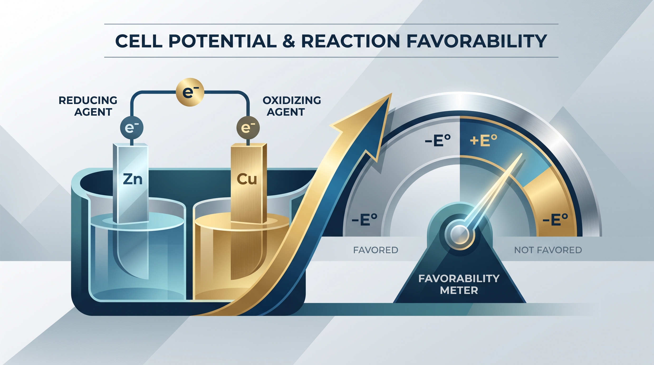
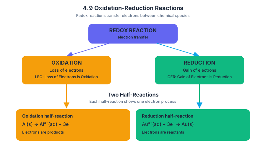
5.1 Reaction Rates · 5.2 Introduction to Rate Law
Key concepts: Reaction rates as changes in reactant or product concentrations over time · Rate law expressions for chemical reactions · Reaction order with respect to an individual reactant · Overall reaction order · Rate constant (k) · Temperature dependence of the rate constant · Units of the rate constant based on overall reaction order · Determining reactant orders by comparing initial rates · First-order kinetics and linear plots of ln(reactant concentration) versus time · Using radioactive decay and crystal violet fading as examples of kinetics
A chemical reaction can be fast enough to inflate a balloon in seconds or slow enough to preserve a radioactive isotope for thousands of years.
5.1 Reaction Rates · 5.2 Introduction to Rate Law
A chemical reaction can be fast enough to inflate a balloon in seconds or slow enough to preserve a radioactive isotope for thousands of years. Reaction rate is the change in concentration of a reactant or product per unit time.
Rate describes how the concentration of a reaction species changes over time.
For a reactant, concentration decreases, so its rate is written with a negative sign; for a product, concentration increases:
$$ \text{rate}=-\frac{\Delta[\text{reactant}]}{\Delta t} \qquad \text{or} \qquad \text{rate}=\frac{\Delta[\text{product}]}{\Delta t} $$
The usual units are molarity per second, written as $\text{M},\text{s}^{-1}$.
From measured rate to rate law
A measured rate tells how fast a reaction is proceeding under particular conditions. A rate law is the equation that connects that rate to the concentrations of reactants and a proportionality constant called the rate constant, $k$:
$$ \text{rate}=k[A]^m[B]^n $$
Here, $[A]$ and $[B]$ are reactant concentrations. The exponents $m$ and $n$ are determined experimentally; they cannot usually be inferred from the coefficients in the balanced chemical equation.
The exponent attached to one reactant is its reaction order with respect to that reactant. Thus, $m$ is the order with respect to $A$, and $n$ is the order with respect to $B$. The overall reaction order is the sum of all concentration exponents:
$$ \text{overall order}=m+n $$
| Rate-law feature | Meaning |
|---|---|
| $[A]^m$ | Order $m$ with respect to $A$ |
| $[B]^n$ | Order $n$ with respect to $B$ |
| $m+n$ | Overall reaction order |
| $k$ | Rate constant at a particular temperature |
Misconception check — coefficients are not automatically orders. For a reaction such as $2A+B\rightarrow C$, the rate law is not automatically $k[A]^2[B]$. Reaction orders come from experimental rate data unless the reaction is known to occur in a single elementary step, a distinction developed later.
Determining orders by comparing initial rates
The method of initial rates determines one reactant’s order by comparing experiments in which that reactant changes while the others remain constant. If doubling $[A]$ doubles the initial rate, the reaction is first-order in $A$; if doubling $[A]$ quadruples the rate, it is second-order in $A$.
Worked example: ascorbic acid and triiodide
Suppose three trials produce the following initial-rate observations:
- Trial 1: $[HA sc]=0.225\ \text{M}$, $[I_3^-]=0.200\ \text{M}$, rate $=1.229\times10^{-4}\ \text{M},\text{s}^{-1}$
- Trial 3: $[HA sc]=0.450\ \text{M}$, $[I_3^-]=0.200\ \text{M}$, rate $=2.457\times10^{-4}\ \text{M},\text{s}^{-1}$
Only $[HA sc]$ doubles, and the rate also doubles:
$$ \frac{\text{rate}_3}{\text{rate}_1}
\left(\frac{[HA sc]_3}{[HA sc]_1}\right)^m $$
$$ 2=2^m\Rightarrow m=1 $$
Therefore, the reaction is first-order with respect to $[HA sc]$. If a second comparison shows that doubling $[I_3^-]$ also doubles the rate, then:
$$ \text{rate}=k[HA sc][I_3^-] $$
Now calculate $k$ using Trial 3:
$$ k=\frac{\text{rate}}{[HA sc][I_3^-]} $$
$$ k= \frac{2.457\times10^{-4}\ \text{M},\text{s}^{-1}} {(0.450\ \text{M})(0.200\ \text{M})} $$
$$ k=2.73\times10^{-3}\ \text{M}^{-1}\text{s}^{-1} $$
The units follow from the equation: $k$ must convert $\text{M}^2$ into $\text{M},\text{s}^{-1}$.
The rate constant and temperature
The rate constant, $k$, measures the proportionality between reactant concentrations and reaction rate. Its numerical value depends on temperature, so a rate law must be understood as applying at a specified temperature. The units of $k$ also depend on the overall reaction order.
$$ \begin{aligned} \text{zero order:}\quad &[k]=\text{M},\text{s}^{-1}\ \text{first order:}\quad &[k]=\text{s}^{-1}\ \text{second order:}\quad &[k]=\text{M}^{-1}\text{s}^{-1} \end{aligned} $$
Misconception check — $k$ is not the same as rate. Rate changes when concentrations change. At fixed temperature, $k$ remains constant for a given reaction and rate-law form; changing temperature changes $k$.
First-order evidence in concentration–time data
For a reaction first-order in a monitored reactant $A$, a plot of $\ln[A]$ against time is linear:
$$ \ln[A]_t-\ln[A]_0=-kt $$
The slope is $-k$. Radioactive decay is a familiar first-order process because the decay rate is proportional to the amount of radioactive material remaining. A constant half-life is another characteristic clue: each successive half-life removes half of what remains, not the same absolute amount.
Crystal violet: seeing kinetics with light
The fading or decomposition of crystal violet provides a direct laboratory investigation of rate law. Because crystal violet absorbs visible light, its concentration can be monitored with a spectrophotometer using Beer’s law:
$$ A=\varepsilon bc $$
At constant path length $b$ and molar absorptivity $\varepsilon$, absorbance $A$ is proportional to concentration $c$. Concentration–time data can therefore be transformed into rate information and tested for the rate law that best describes the reaction.
This investigation connects a visible phenomenon—purple color fading—to particle-level kinetics and mathematical evidence. It develops LO 5.2.A, especially EK 5.2.A.1–5.2.A.5: interpreting rate laws, identifying individual and overall reaction orders, relating units to order, recognizing the temperature dependence of $k$, and using initial-rate comparisons.
The principal AP skill is Skill 5.C: Mathematical Routines — Explain the relationship between variables within an equation when one variable changes. A strong response does not merely state “first-order”; it identifies what was held constant, compares concentration and rate ratios, and explains why the observed proportionality gives the exponent.
Retrieval check. If doubling $[A]$ leaves the rate unchanged, what is the order with respect to $A$? If doubling $[A]$ makes the rate eight times larger, what is the order? Answers: zero order and third order, because $2^0=1$ and $2^3=8$.
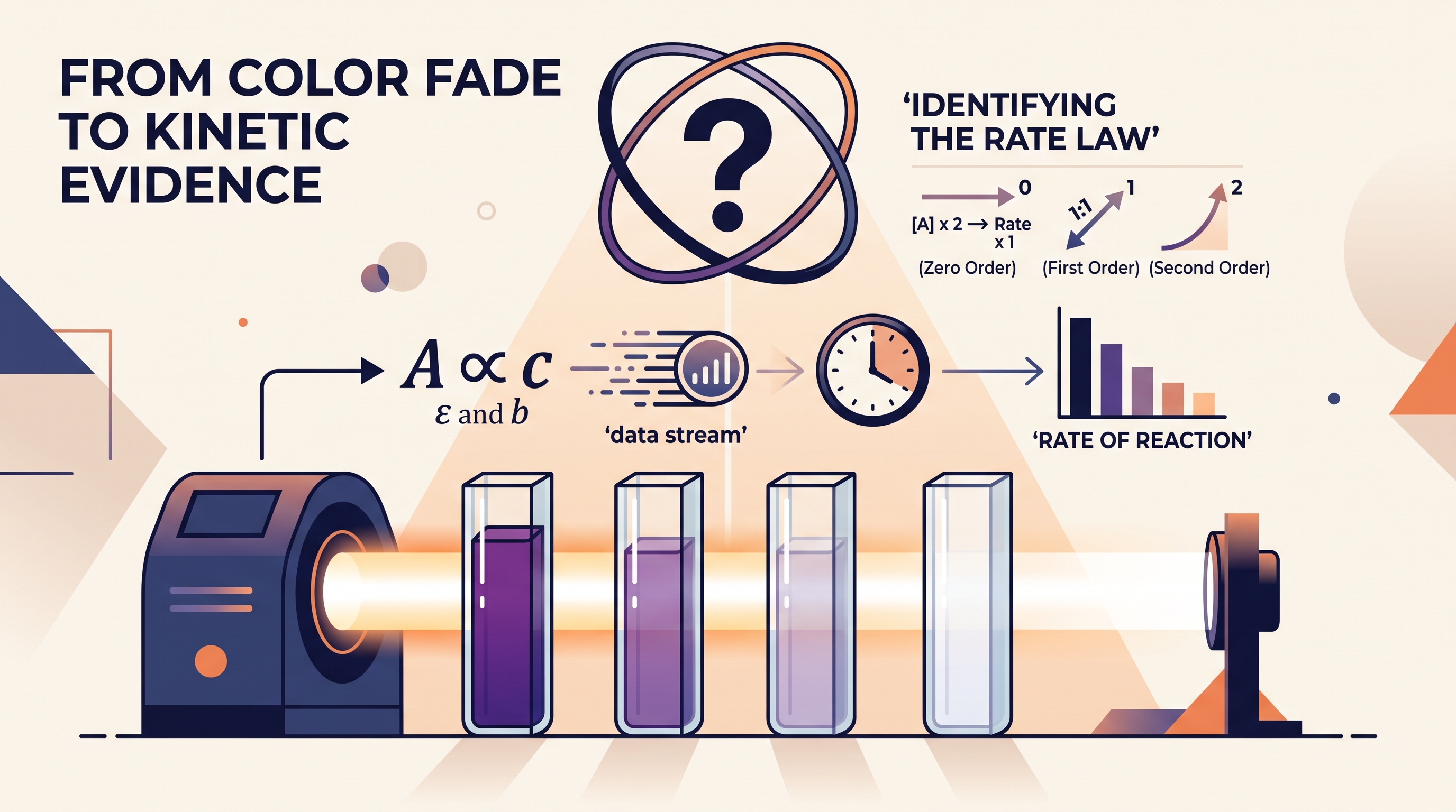
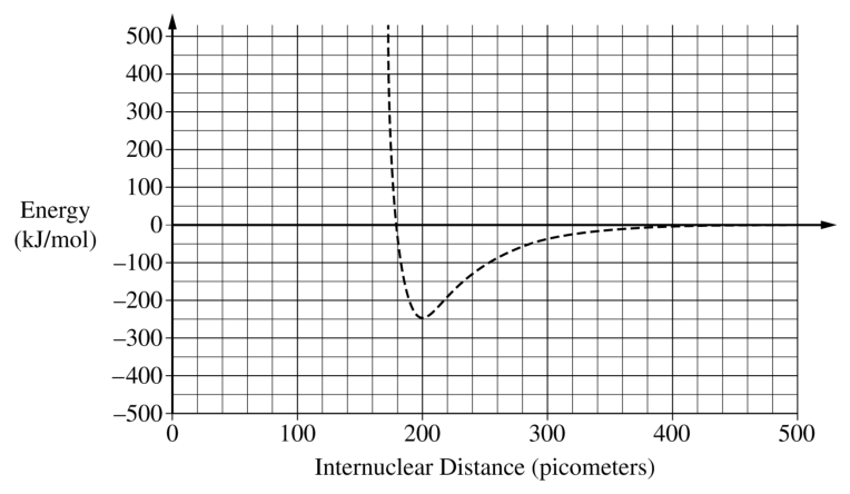
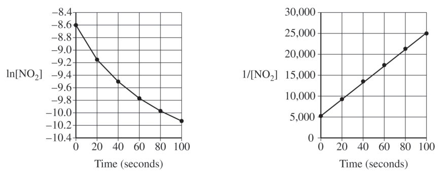
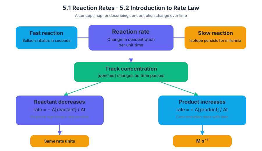
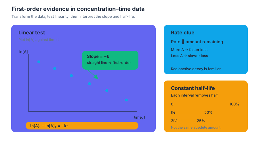
5.3 Concentration Changes Over Time · 5.4 Elementary Reactions
Key concepts: Concentration changes over time · Integrated rate laws for zeroth-, first-, and second-order reactions · Reaction order and rate constant · Slopes of concentration-versus-time data · Beer’s Law and spectrophotometry · Fading of crystal violet as a kinetics investigation · Determining rate laws from experimental evidence · Reaction mechanisms and intermediates · Catalysts and the rate-determining step · Energy profiles for chemical reactions
A reaction’s changing concentration is a chemical clock: the shape of the data reveals the reaction order, the slope reveals the rate constant, and the mechanism explains which molecular event controls the observed rate.
5.3 Concentration Changes Over Time · 5.4 Elementary Reactions
A reaction’s changing concentration is a chemical clock: the shape of the data reveals the reaction order, the slope reveals the rate constant, and the mechanism explains which molecular event controls the observed rate.
From concentration data to reaction order
For a reactant $A$, concentration-versus-time data show how quickly $[A]$ decreases. The decisive test is not merely whether the graph slopes downward, but which transformation of concentration produces a straight line.
| Reaction order in $A$ | Linear graph | Integrated rate law | Meaning of slope |
|---|---|---|---|
| Zeroth order | $[A]$ versus $t$ | $[A]_t-[A]_0=-kt$ | $-k$ |
| First order | $\ln[A]$ versus $t$ | $\ln[A]_t-\ln[A]_0=-kt$ | $-k$ |
| Second order | $1/[A]$ versus $t$ | $\frac{1}{[A]_t}-\frac{1}{[A]_0}=kt$ | $+k$ |
These relationships preserve the essential knowledge statements 5.3.A.1, 5.3.A.2, 5.3.A.3, and 5.3.A.4: reaction order can be inferred from concentration data; a first-order reaction gives a linear $\ln[A]$-versus-time plot; a second-order reaction gives a linear $1/[A]$-versus-time plot; and the slope supplies the rate constant.
Worked example: identifying order and $k$
Suppose a reactant has the following measured concentrations:
| $t$ in $s$ | $[A]$ in $M$ | $\ln[A]$ | $1/[A]$ in $M^{-1}$ |
|---|---|---|---|
| $0$ | $0.100$ | $-2.303$ | $10.0$ |
| $20$ | $0.0500$ | $-2.996$ | $20.0$ |
| $40$ | $0.0250$ | $-3.689$ | $40.0$ |
The concentration halves every $20\ \mathrm{s}$. More decisively, $\ln[A]$ decreases by approximately $0.693$ during each equal time interval, so $\ln[A]$ versus $t$ is linear. The reaction is first order, and
$$ k=-\text{slope} =-\frac{-2.996-(-2.303)}{20\ \mathrm{s}} =3.47\times10^{-2}\ \mathrm{s^{-1}}. $$
The first-order integrated law predicts the concentration at $t=60\ \mathrm{s}$:
$$ \ln[A]_{60}-\ln(0.100) =-(3.47\times10^{-2})(60), $$
$$ [A]_{60}=0.0125\ \mathrm{M}. $$
Misconception check — “The steepest concentration graph identifies the order.” It does not. A graph of $[A]$ versus $t$ can curve for a first- or second-order reaction, and its visual steepness depends on the starting concentration and units. Test $[A]$, $\ln[A]$, and $1/[A]$ systematically.
Half-life and units of $k$
A half-life, $t_{1/2}$, is the time required for a reactant concentration to fall to one-half its current value. For a first-order reaction, the half-life is constant:
$$ t_{1/2}=\frac{\ln 2}{k}. $$
For the worked example,
$$ t_{1/2}=\frac{0.693}{3.47\times10^{-2}\ \mathrm{s^{-1}}} =20.0\ \mathrm{s}. $$
This constancy is diagnostic: equal concentration-halving intervals support first-order behavior. The units of $k$ depend on overall reaction order: $\mathrm{s^{-1}}$ for first order, $\mathrm{M,s^{-1}}$ for zeroth order, and $\mathrm{M^{-1},s^{-1}}$ for second order. Misconception check — “$k$ always has units of $\mathrm{s^{-1}}$.” Only a first-order rate constant does.
Beer’s law: turning color into concentration
Spectrophotometry measures how strongly a solution absorbs light. Beer’s law connects absorbance, $A_{\mathrm{abs}}$, to concentration:
$$ A_{\mathrm{abs}}=\varepsilon bc, $$
where $\varepsilon$ is the molar absorptivity, $b$ is the path length of the cuvette, and $c$ is concentration. If $\varepsilon$ and $b$ remain constant, absorbance is directly proportional to concentration.
In the fading crystal violet investigation, the purple reactant becomes less concentrated as the reaction proceeds, so its absorbance decreases. A calibration relationship—or a constant proportionality when conditions permit—converts each absorbance measurement into $[\mathrm{CV}^+]$. The resulting concentration data can then be tested using $[A]$, $\ln[A]$, and $1/[A]$ plots.
Experimental reasoning chain:
- Measure absorbance at successive times.
- Convert absorbance to concentration using Beer’s law.
- Construct the three linearized plots.
- Select the plot with the best linear pattern.
- Use its slope to determine $k$.
- Check whether the calculated half-life agrees with the concentration data.
5.4 Elementary reactions and mechanisms
An elementary reaction is a single molecular event. Its rate law follows directly from the reacting particles in that step, unlike the experimentally determined rate law for an overall reaction, which may require evidence from several trials.
For a proposed mechanism, an intermediate is formed in one elementary step and consumed in a later step, so it cancels when the steps are added. A catalyst is consumed in an early step and regenerated later; it participates in the mechanism but does not appear in the net reaction.
The rate-determining step is the slow step that limits the overall rate. A valid mechanism must satisfy two tests: its elementary steps must add to the observed overall equation, and its predicted rate behavior must agree with the experimentally constructed rate law. A mechanism that balances atoms but predicts the wrong dependence on concentration is rejected.
For example, consider
$$ A+B\longrightarrow I $$
followed by
$$ I+C\longrightarrow P. $$
Here $I$ is an intermediate because it is produced and then consumed. Adding the steps gives
$$ A+B+C\longrightarrow P. $$
The mechanism must be checked against the measured rate law rather than accepted from stoichiometric balancing alone.
Science Practice 5: Mathematical Routines is central to Topics 5.3 and 5.4: transform data, calculate slopes and half-lives, track units, and use equations to test mechanisms. Science Practice 3: Representing Data and Phenomena also enters whenever concentration changes, spectrophotometric measurements, graphs, or mechanism diagrams are translated into chemical meaning.
Energy profiles for mechanisms are constructed and analyzed with the reaction-energy ideas developed in 5.6 Reaction Energy Profile; here, the essential mechanistic task is identifying elementary steps, intermediates, catalysts, and the rate-determining step without confusing a proposed pathway with experimental proof.
Retrieval check: A plot of $1/[A]$ versus time is linear with slope $0.080\ \mathrm{M^{-1},s^{-1}}$. What is the reaction order, and what happens to $[A]$ after one half-life? Answer: It is second order, $k=0.080\ \mathrm{M^{-1},s^{-1}}$, and the concentration becomes one-half its initial value; unlike a first-order reaction, successive second-order half-lives are not generally equal.
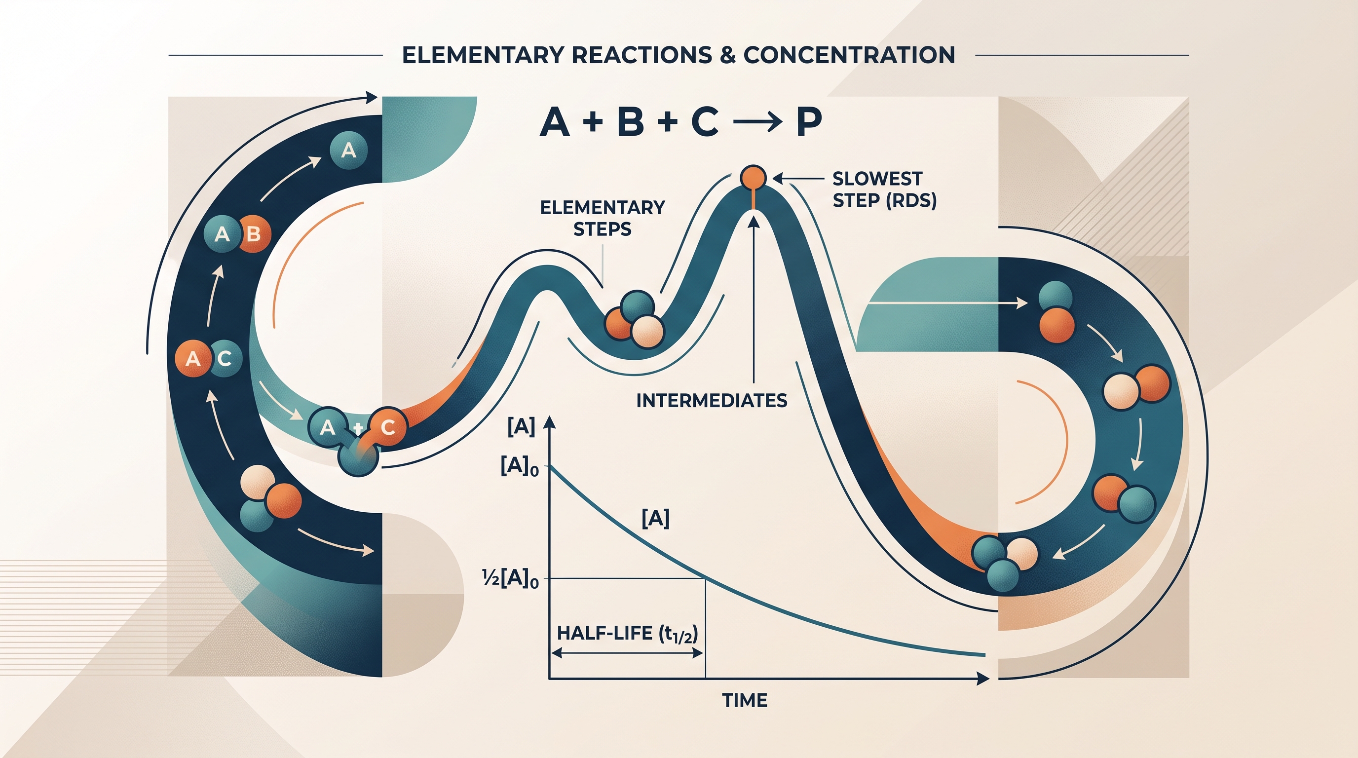
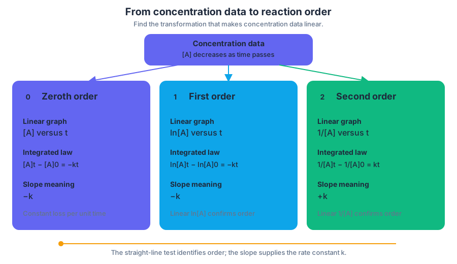
5.5 Collision Model · 5.6 Reaction Energy Profile
Key concepts: Collision model · Successful collisions · Activation energy (Ea) · Bond breaking and bond making · Reaction energy profile · Energy changes along a reaction pathway · Enthalpy change (ΔH) · Connection between particulate and macroscopic scales · Scientific argumentation (6.E) · Reaction rates and kinetics
A chemical reaction begins when reactant particles collide in a way that allows old bonds to break and new bonds to form—but most collisions fail.
5.5 Collision Model · 5.6 Reaction Energy Profile
A chemical reaction begins when reactant particles collide in a way that allows old bonds to break and new bonds to form—but most collisions fail. The collision model connects these microscopic events to the macroscopic reaction rate, the observable speed at which reactants disappear and products appear.
5.5 Collision Model: What makes a collision successful?
Imagine two puzzle pieces moving across a table. A collision does not guarantee that they will connect: they must meet often enough, hit with enough energy, and approach with compatible shapes. Reacting particles behave similarly. For an elementary reaction, reactant particles must collide with the correct frequency, sufficient energy, and suitable orientation.
5.5.A.1: For an elementary reaction to successfully produce products, reactants must successfully collide to initiate bond-breaking and bond-making events.
A successful collision is a collision that produces products. It must satisfy three conditions:
- Frequency: More collisions per unit time create more opportunities for reaction.
- Energy: The particles must have enough kinetic energy to overcome the activation-energy requirement.
- Orientation: The particles must strike in a geometric arrangement that permits the necessary bonds to break and form.
This explains why increasing concentration often increases reaction rate: more particles occupy the same volume, so collisions occur more frequently. Increasing temperature affects both particle motion and the fraction of collisions energetic enough to react. Changing the orientation requirement changes the probability that a collision has the correct geometry.
Connecting the particulate and macroscopic scales
The reaction rate measured in a laboratory is a macroscopic observation. The collision model explains that observation using microscopic reasoning: a faster reaction corresponds to a greater number of successful collisions per unit time.
Science Practice 6.E — Argumentation: Provide reasoning to justify a claim using connections between particulate and macroscopic scales or levels.
Worked argument: A powdered solid reacts faster than the same mass of large pieces. At the particulate level, powder exposes more surface area, allowing more particles at the solid’s surface to collide with particles in the other reactant. The collision frequency therefore increases, producing more successful collisions per unit time and a greater macroscopic reaction rate.
Notice the logic: the claim is not merely “powder reacts faster.” The justification connects surface-level particle access to collision frequency, then connects collision frequency to observable rate. A response that names only the macroscopic trend does not fully establish the chemical reason.
Activation energy and the transition state
Activation energy, written $E_a$, is the minimum energy required for colliding particles to reach the transition state—the unstable arrangement at the highest-energy point along the reaction pathway. During this brief event, bonds are being broken and formed simultaneously.
Particles can collide frequently and still react slowly if very few collisions have energy greater than or equal to $E_a$. This is why “more collisions” and “more successful collisions” are not identical ideas.
Common misconception — “Every collision causes a reaction.”
Collision is necessary, but it is not sufficient. A collision must have adequate energy and appropriate orientation; only a small fraction of collisions leads to products.
5.6 Reaction Energy Profile: Mapping the pathway
A reaction energy profile shows how energy changes as reactants are rearranged into products. The horizontal axis is the reaction coordinate, an abstract measure of progress through the complex motions involved in the rearrangement. The vertical axis represents the energy of the reacting system.
For a single elementary reaction, the profile normally has three essential regions:
- Reactants: the starting energy level.
- Transition state: the peak, where the bonds are in the highest-energy unstable arrangement.
- Products: the ending energy level after new bonds have formed.
The vertical difference from the reactants to the peak is the activation energy for the forward reaction:
$$ E_a = E_{\text{transition state}} - E_{\text{reactants}} $$
The vertical difference between products and reactants is the overall enthalpy change:
$$ \Delta H = E_{\text{products}} - E_{\text{reactants}} $$
If the products lie below the reactants, $\Delta H < 0$ and the reaction is exothermic: the system releases energy overall. If the products lie above the reactants, $\Delta H > 0$ and the reaction is endothermic: the system absorbs energy overall. In either case, the reaction may require a positive $E_a$ to begin.
Profile-labeling example: Suppose the reactants are at $40\ \mathrm{kJ,mol^{-1}}$, the transition state is at $115\ \mathrm{kJ,mol^{-1}}$, and the products are at $10\ \mathrm{kJ,mol^{-1}}$.
$$ E_a = 115 - 40 = 75\ \mathrm{kJ,mol^{-1}} $$
$$ \Delta H = 10 - 40 = -30\ \mathrm{kJ,mol^{-1}} $$
The reaction is exothermic, but it still requires $75\ \mathrm{kJ,mol^{-1}}$ of activation energy to reach the transition state.
Common misconception — “Exothermic means spontaneous and fast.” Exothermicity describes the sign of $\Delta H$, not the speed of the reaction. A reaction can release energy overall and still be extremely slow if its $E_a$ is large. Conversely, lowering $E_a$ changes the rate without changing the overall $\Delta H$.
Temperature and the energy barrier
When temperature increases, the proportion of particle collisions energetic enough to reach the transition state increases. The reaction rate therefore increases because a larger fraction of collisions can become successful—not because the activation energy itself changes.
The Arrhenius equation models this temperature dependence:
$$ k = A e^{-E_a/(RT)} $$
Here, $k$ is the rate constant, $A$ represents collision frequency and orientation effects, $E_a$ is the activation energy, $R$ is the gas constant, and $T$ is absolute temperature in kelvins. At AP Chemistry level, the essential interpretation is graphical and conceptual: temperature changes the fraction of collisions that can cross the energy barrier.
Retrieval check
A reaction profile has reactants at $80\ \mathrm{kJ,mol^{-1}}$, a peak at $140\ \mathrm{kJ,mol^{-1}}$, and products at $105\ \mathrm{kJ,mol^{-1}}$. What are $E_a$ and $\Delta H$? Is the reaction exothermic or endothermic? Explain, in one sentence, how a higher temperature changes the number of successful collisions.
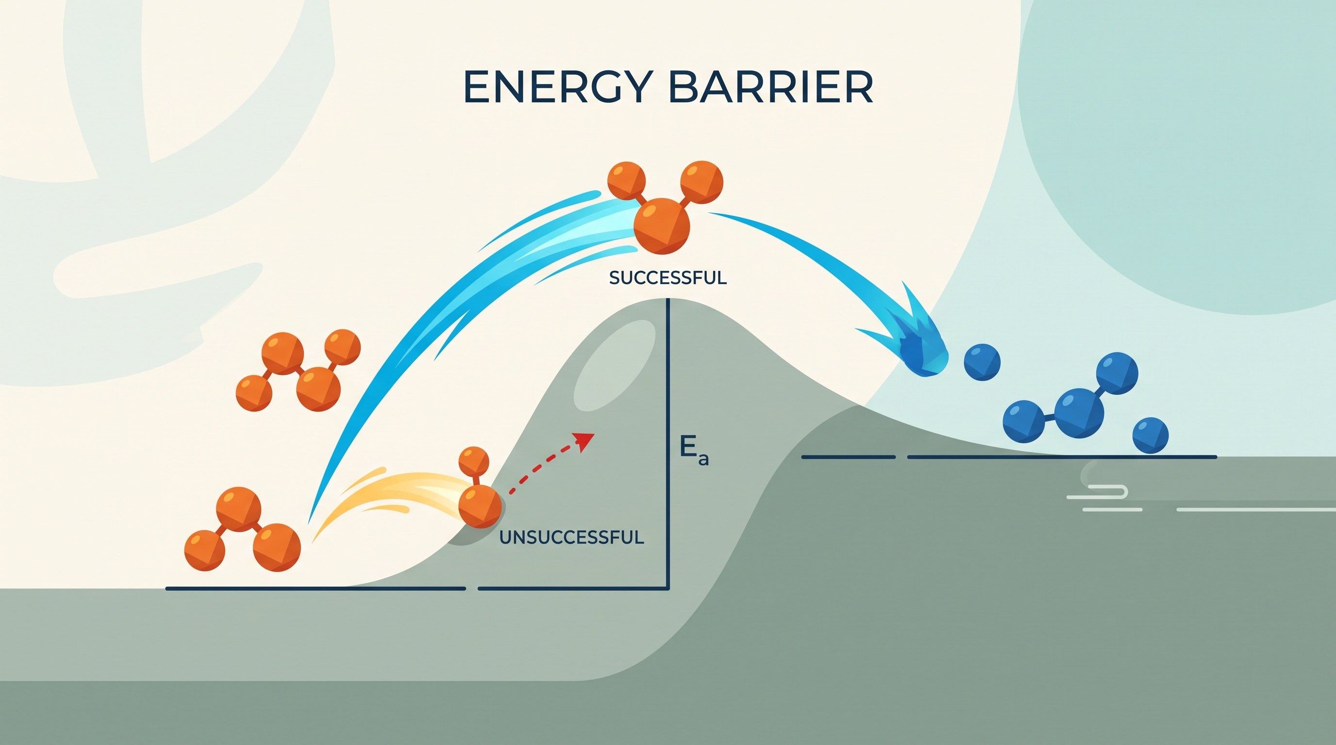
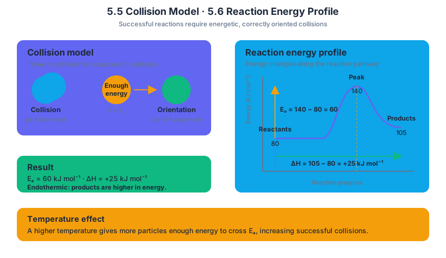
5.7 Introduction to Reaction Mechanisms · 5.8 Reaction Mechanism and Rate Law
Key concepts: Reaction mechanisms as sequences of elementary reactions · Relating experimental rate data, rate laws, and proposed mechanisms · Identifying a rate law from a mechanism when the first elementary step is rate limiting · Rate-limiting steps and their effect on the overall rate law · Evaluating whether a proposed mechanism is consistent with an observed rate law · Catalysts changing reaction mechanisms · Catalysts providing an alternative pathway with lower activation energy · Effective collisions and activation energy · Mathematical routines for identifying appropriate rate laws and relationships · Acid-base equilibrium constants in reaction examples
A reaction mechanism is a sequence of elementary reactions that shows how reactant particles are transformed into products one molecular event at a time. The experimentally measured rate law is a powerful test of whether that proposed sequence is chemically credible.
5.7 Introduction to Reaction Mechanisms · 5.8 Reaction Mechanism and Rate Law
A reaction mechanism is a sequence of elementary reactions that shows how reactant particles are transformed into products one molecular event at a time. The experimentally measured rate law is a powerful test of whether that proposed sequence is chemically credible.
From one equation to several elementary steps
An overall equation hides the pathway. For example, the net reaction
$$ A+B\rightarrow D $$
might occur through
$$ \text{Step 1: } A+B\rightarrow I $$
$$ \text{Step 2: } I\rightarrow D $$
where $I$ is an intermediate: a species formed in one step and consumed in a later step. Adding the elementary steps cancels $I$, leaving the overall equation. An intermediate therefore appears in the mechanism but not in the net reaction.
An elementary reaction represents a single molecular event. Its rate law follows directly from the particles involved in that event, so the coefficients of the reactants become the exponents in that elementary-step rate law. This connection is called the step’s molecularity.
Essential Knowledge 5.8.A.1: For mechanisms in which each elementary step is irreversible, or in which the first step is rate limiting, the rate law is set by the molecularity of the slowest elementary step.
The rate-limiting first step
The rate-limiting step is the slowest elementary step in a proposed mechanism. It acts like a narrow doorway: even if later steps are fast, the overall process cannot proceed faster than particles pass through that bottleneck.
For Learning Objective 5.8.A, the required case is a mechanism in which the first elementary step is rate limiting. In that specific situation, the overall rate law is based on the reactants in the first step.
Worked example: identifying the rate law
Suppose a proposed mechanism is
$$ \text{Step 1: } 2X+Y\rightarrow I \qquad \text{slow} $$
$$ \text{Step 2: } I\rightarrow Z \qquad \text{fast} $$
The first step is rate limiting, so write its elementary rate law:
$$ \text{rate}=k[X]^2[Y] $$
The predicted overall reaction rate law is therefore
$$ \boxed{\text{rate}=k[X]^2[Y]} $$
The exponents come from the coefficients of $X$ and $Y$ in the slow elementary step—not from the coefficients in the overall equation. If doubling $[X]$ increases the rate by a factor of $4$, while doubling $[Y]$ doubles the rate, those observations support second order in $X$ and first order in $Y$.
Misconception check — “Balance the overall equation, then copy its coefficients into the rate law.” Overall-equation coefficients generally do not determine reaction orders. Reaction orders must come from experimental data or, in the specially permitted mechanism shortcut, from the molecularity of the rate-limiting elementary step.
Testing a proposed mechanism against data
A mechanism must satisfy two independent requirements:
- Its elementary steps must add to the observed overall chemical equation.
- Its predicted rate law must agree with the experimentally observed rate law.
For example, suppose experimental trials show that doubling $[A]$ doubles the rate, while doubling $[B]$ leaves the rate unchanged. The observed law is
$$ \text{rate}=k[A] $$
A proposed first-step-limiting mechanism beginning with
$$ A+B\rightarrow I \qquad \text{slow} $$
would predict
$$ \text{rate}=k[A][B] $$
Because the prediction includes $[B]$, it conflicts with the data. The mechanism may still produce the correct overall equation, but it is not consistent with the observed kinetics.
When data are tabulated, compare rate ratios rather than merely comparing raw rates. When data are graphed, inspect how the rate responds as one reactant concentration changes while the others remain controlled. This uses Skill 5.B: Identify an appropriate theory, definition, or mathematical relationship to solve a problem: select the elementary-step rate relationship that matches the stated rate-limiting condition, then test it against evidence.
When the shortcut does not apply
The rule “the slow step gives the rate law” is not a universal shortcut. It applies directly here when the first elementary step is rate limiting, or under the stated additional conditions involving irreversible elementary steps. If the first step is fast and reversible, an intermediate may appear in the rate expression; determining its concentration requires an approximation such as pre-equilibrium treatment, which belongs to the later rate-law analysis.
Important scope: The AP Chemistry exam does not assess collecting experimental data to detect a reaction intermediate. It does assess using a given mechanism, rate data, equations, and representations to judge whether the mechanism explains observed behavior.
Catalysts create a different pathway
A catalyst increases reaction rate by changing the mechanism, not by changing the overall reaction. It may increase the number of effective collisions or provide a pathway with a lower activation energy. Because the catalyst is regenerated, it does not appear in the net equation.
For a simple catalytic mechanism,
$$ \text{Step 1: } R+C\rightarrow RC $$
$$ \text{Step 2: } RC\rightarrow P+C $$
adding the steps cancels $C$:
$$ R\rightarrow P $$
The catalyst $C$ can be consumed in one elementary step and regenerated in another. Its concentration may remain essentially constant even though it participates directly in the pathway.
Misconception check — “A catalyst makes a reaction more favorable.” A catalyst changes the route and lowers the kinetic barrier; it does not change the overall reactants, products, or thermodynamic equilibrium constant. It changes how fast equilibrium is reached, not the final equilibrium composition.
Retrieval check
A mechanism begins with the slow elementary step
$$ M+2N\rightarrow I $$
and experimental data show first order in $M$ and second order in $N$. The predicted rate law is
$$ \boxed{\text{rate}=k[M][N]^2} $$
This mechanism passes the rate-law test only if its elementary steps also add to the observed overall equation. Why would a catalyst not appear in that overall equation? Because it is regenerated and cancels when the mechanism’s steps are added.
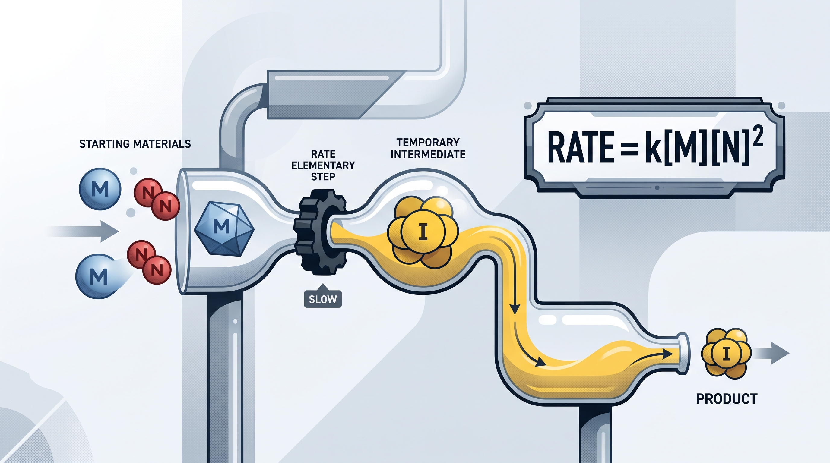
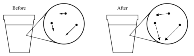
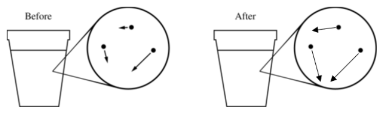
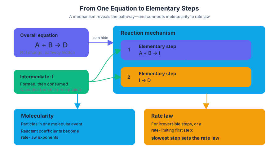
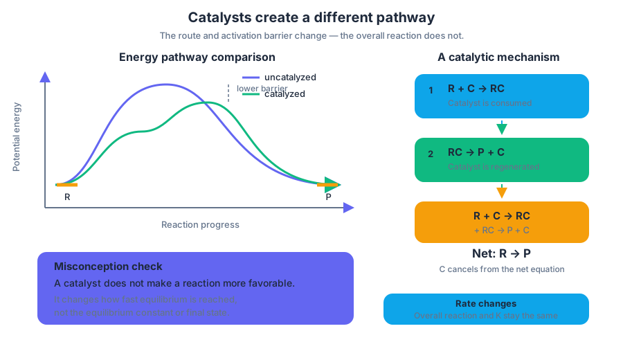
5.9 Pre-Equilibrium Approximation · 5.10 Multistep Reaction Energy Profile
Key concepts: Pre-equilibrium approximation · Multistep reaction energy profiles · Activation energy · Overall energy change · Elementary reactions · Reaction mechanisms · Energetics of elementary reactions · Reaction energy profiles · Unit 5: Kinetics
A reaction can move quickly through a reversible first step, briefly building an intermediate, and then proceed slowly through a later step. The pre-equilibrium approximation uses that temporary equilibrium to express the concentration of the intermediate in terms of measurable reactant concentrations.
5.9 Pre-Equilibrium Approximation · 5.10 Multistep Reaction Energy Profile
A reaction can move quickly through a reversible first step, briefly building an intermediate, and then proceed slowly through a later step. The pre-equilibrium approximation uses that temporary equilibrium to express the concentration of the intermediate in terms of measurable reactant concentrations.
Pre-equilibrium approximation: turning an intermediate into a rate law
Consider the mechanism
A+B \rightleftharpoons I
$$ I+C \longrightarrow P $$
Here, $I$ is an intermediate: it is formed in one elementary reaction and consumed in another, so it does not appear in the overall reaction. If the first step is fast and reversible while the second step is slow, the first step can establish a pre-equilibrium before much product forms.
For the fast reversible step, write the equilibrium expression
$$ K_{\mathrm{pre}}=\frac{[I]}{[A][B]} $$
and solve for the intermediate concentration:
$$ [I]=K_{\mathrm{pre}}[A][B] $$
The slow elementary step determines the reaction rate:
$$ \text{rate}=k_2[I][C] $$
Substituting the pre-equilibrium expression gives
$$ \text{rate}=k_2K_{\mathrm{pre}}[A][B][C] $$
Thus, the experimentally observed rate law can contain $[A]$, $[B]$, and $[C]$, even though the intermediate $I$ never appears in the final rate law.
The key reasoning chain is:
$$ \text{fast reversible step} \longrightarrow \text{equilibrium expression for }[I] \longrightarrow \text{slow-step rate law} \longrightarrow \text{substitution} $$
This is not the same as assuming that every mechanism is at equilibrium. Only the designated fast reversible portion is treated as being in equilibrium.
Conditions and misconception check
Named misconception — “The slow step always gives the final rate law directly.” The slow step gives the rate law in terms of the species participating in that elementary step. If that step contains an intermediate, the intermediate concentration must be replaced using the pre-equilibrium relationship.
Named misconception — “Pre-equilibrium means the entire reaction has reached equilibrium.” It does not. Reactants may still be steadily converted into products. The approximation concerns a rapidly equilibrating early step, while the slower step continues to drain the intermediate toward products.
The approximation becomes unreliable when the first step does not establish equilibrium rapidly relative to the step that consumes the intermediate, or when the assumed slow step is not actually rate-controlling. Always check that the proposed mechanism and approximation are chemically consistent with the observed rate law.
From elementary reactions to an energy profile
A reaction energy profile plots chemical potential energy vertically against reaction progress horizontally. A single elementary reaction has one energy barrier: the peak represents the transition state, and the vertical distance from the reactants to that peak is the activation energy, $E_a$.
A multistep reaction energy profile is different from a general one-step profile because it displays the energetic sequence of several elementary reactions in a mechanism. Each additional elementary step contributes another peak and, usually, another valley.
For a mechanism
$$ R \longrightarrow I_1 \longrightarrow I_2 \longrightarrow P $$
the profile contains:
- the initial reactants, $R$;
- a peak for the transition state of step 1;
- the intermediate $I_1$;
- a peak for step 2;
- the intermediate $I_2$;
- a peak for step 3;
- the final products, $P$.
Each valley between peaks represents an intermediate, not a transition state.
Reading activation energy and overall energy change
Learning Objective 5.10.A: Represent the activation energy and overall energy change in a multistep reaction with a reaction energy profile.
Essential Knowledge 5.10.A.1: Knowledge of the energetics of each elementary reaction in a mechanism allows for the construction of an energy profile for a multistep reaction.
For every elementary step, measure activation energy from that step’s starting valley to its next peak:
$$ E_{a,1}=E_{\mathrm{TS1}}-E_R $$
$$ E_{a,2}=E_{\mathrm{TS2}}-E_{I_1} $$
The overall energy change is measured only from the initial reactants to the final products:
$$ \Delta E_{\mathrm{overall}}=E_P-E_R $$
If the products lie lower than the reactants, the overall reaction is energy-releasing; if they lie higher, it is energy-absorbing. The intermediate valleys affect the route but do not determine the overall energy change.
Worked profile interpretation. Suppose a multistep profile assigns the relative energies
$$ E_R=20\ \mathrm{kJ,mol^{-1}},\quad E_{I_1}=50\ \mathrm{kJ,mol^{-1}},\quad E_{\mathrm{TS1}}=90\ \mathrm{kJ,mol^{-1}} $$
$$ E_{I_2}=35\ \mathrm{kJ,mol^{-1}},\quad E_{\mathrm{TS2}}=75\ \mathrm{kJ,mol^{-1}},\quad E_P=-10\ \mathrm{kJ,mol^{-1}} $$
Then
$$ E_{a,1}=90-20=70\ \mathrm{kJ,mol^{-1}} $$
and
$$ E_{a,2}=75-50=25\ \mathrm{kJ,mol^{-1}} $$
while
$$ \Delta E_{\mathrm{overall}}=-10-20=-30\ \mathrm{kJ,mol^{-1}} $$
The reaction has a large first barrier but an overall energy decrease of $30\ \mathrm{kJ,mol^{-1}}$. Those are different quantities.
Skill focus: constructing the model
Suggested Skill 3.B: Representing Data and Phenomena means representing chemical substances or phenomena with appropriate diagrams or models. For a multistep profile, an effective model must show the relative energy of reactants, products, intermediates, and transition states; include one peak for each elementary reaction; label relevant activation energies; and show the overall energy change between the starting and ending species.
Named misconception — “The highest point is always the activation energy.” The highest point is a transition-state energy. An activation energy is a difference between a transition-state energy and the energy of the species immediately before that step. The overall rate-controlling barrier is identified by the largest relevant activation-energy difference, not merely by the peak with the greatest absolute height.
Retrieval check: A profile begins at $40\ \mathrm{kJ,mol^{-1}}$, reaches a first peak at $100\ \mathrm{kJ,mol^{-1}}$, falls to an intermediate at $60\ \mathrm{kJ,mol^{-1}}$, rises to a second peak at $120\ \mathrm{kJ,mol^{-1}}$, and ends at $10\ \mathrm{kJ,mol^{-1}}$. The answers are $E_{a,1}=60\ \mathrm{kJ,mol^{-1}}$, $E_{a,2}=60\ \mathrm{kJ,mol^{-1}}$, and $\Delta E_{\mathrm{overall}}=-30\ \mathrm{kJ,mol^{-1}}$. The equal activation energies do not make the two steps identical: their intermediates, molecular changes, and rate constants may still differ.
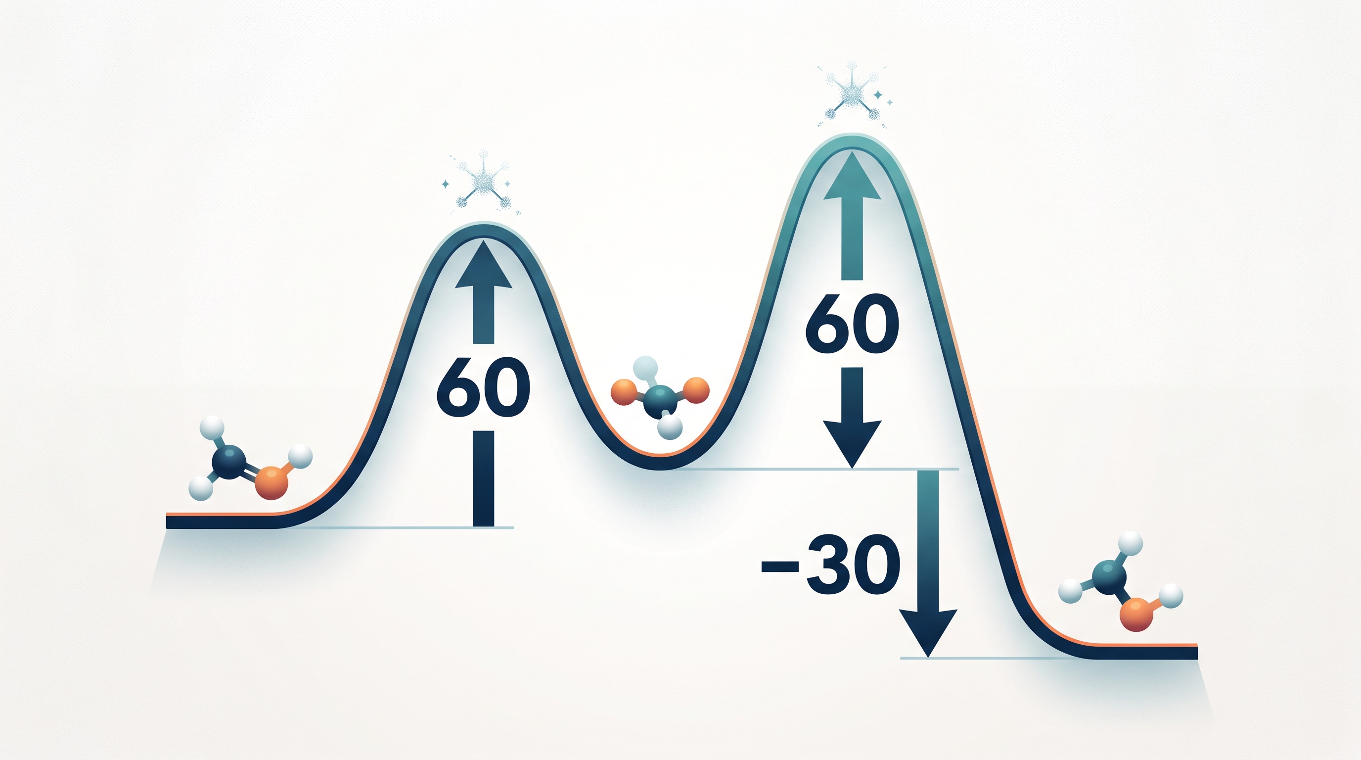
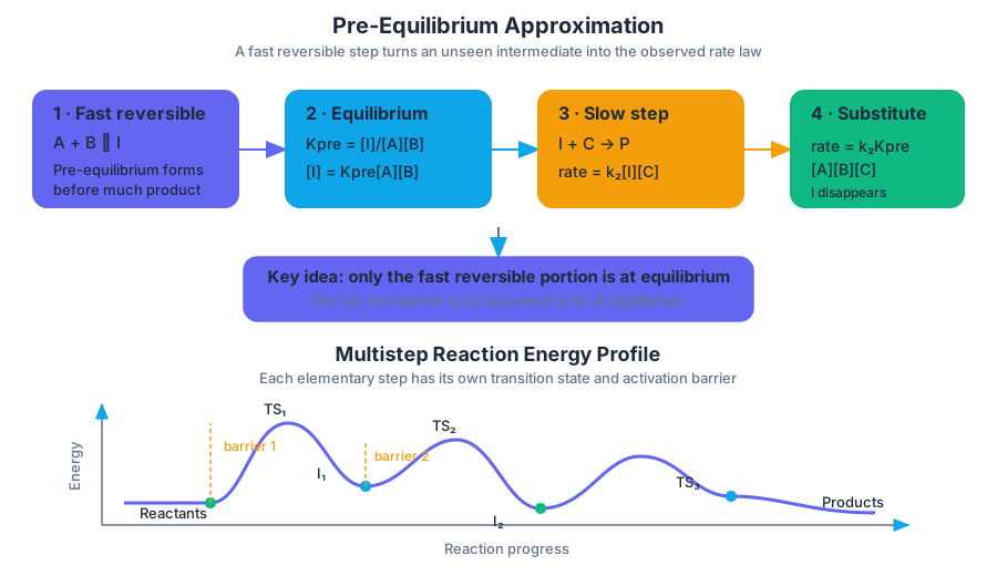
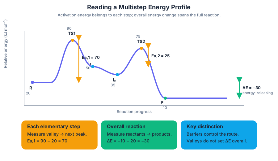
5.11 Catalysis
A catalyst increases the rate of a chemical reaction by providing an alternative reaction pathway with a lower activation energy, $E_a$. It changes how fast a reaction reaches equilibrium, not the final equilibrium composition or the overall energy change of the reaction.
5.11 Catalysis
A catalyst increases the rate of a chemical reaction by providing an alternative reaction pathway with a lower activation energy, $E_a$. It changes how fast a reaction reaches equilibrium, not the final equilibrium composition or the overall energy change of the reaction.
Imagine a mountain pass between two valleys. Reactants occupy one valley and products occupy the other. A catalyst does not move either valley up or down; it creates a lower pass between them. More particles can cross the lower pass successfully, so the reaction proceeds faster.
The energy picture
For a reaction, the activation energy is the minimum energy required for reactant particles to reach the transition state. On an energy diagram, a catalyzed pathway has a smaller peak than the uncatalyzed pathway.
$$ E_a = E_{\text{transition state}} - E_{\text{reactants}} $$
The catalyst may participate in one or more elementary steps, but it is regenerated by the end of the mechanism. Therefore, it appears as a reactant in one step and a product in another, then cancels when the elementary steps are added to obtain the overall reaction.
For example, suppose a catalyst, $C$, changes the reaction
$$ A + B \rightarrow D $$
into the two-step mechanism
$$ A + C \rightarrow AC $$
$$ AC + B \rightarrow D + C $$
Adding the steps gives
$$ A + B + C \rightarrow D + C $$
Because $C$ appears on both sides, it cancels:
$$ A + B \rightarrow D $$
The catalyst is not consumed in the net reaction, even though it is chemically involved in the mechanism.
What catalysis changes—and what it does not
| Quantity | Effect of adding a catalyst |
|---|---|
| Forward reaction rate | Increases |
| Reverse reaction rate | Increases |
| Activation energy | Decreases through an alternative pathway |
| Overall enthalpy change, $\Delta H$ | Unchanged |
| Overall Gibbs free-energy change, $\Delta G$ | Unchanged |
| Equilibrium constant, $K$ | Unchanged |
| Time required to reach equilibrium | Decreases |
| Equilibrium concentrations | Unchanged |
A catalyst accelerates both the forward and reverse reactions because it provides a lower-energy pathway in either direction. The system therefore reaches equilibrium sooner, but the catalyst does not shift the equilibrium position. Since $K$ depends on thermodynamic properties at a given temperature—not on the reaction pathway—the value of $K$ remains constant.
Key distinction: A catalyst changes kinetics, the speed and pathway of a reaction. It does not change thermodynamics, the energy difference between reactants and products.
Worked contextual example: catalytic decomposition
Hydrogen peroxide decomposes slowly according to
$$ 2H_2O_2(aq) \rightarrow 2H_2O(l) + O_2(g) $$
A catalyst such as iodide ion can increase the rate of oxygen formation. If the uncatalyzed pathway has an activation energy of $75\ \text{kJ mol}^{-1}$ and the catalyzed pathway has an activation energy of $42\ \text{kJ mol}^{-1}$, the catalyst lowers the barrier by
$$ \Delta E_a = 75 - 42 = 33\ \text{kJ mol}^{-1} $$
The reaction produces oxygen more rapidly, but the catalyst does not alter the reaction enthalpy. It also does not cause more total oxygen to form at equilibrium; it merely allows the system to approach that equilibrium more quickly.
Reasoning used: identify the catalyst from the mechanism or context, compare the activation-energy barriers, and separate rate information from equilibrium or energy-change information. A claim that “the catalyst makes the reaction more favorable” is incomplete or incorrect unless “favorable” is being used only to describe the lower kinetic barrier.
Catalysts in mechanisms
A catalyst can be homogeneous, meaning it is in the same phase as the reactants, or heterogeneous, meaning it is in a different phase. A solid metal surface, for example, can provide locations where gas molecules adsorb, bonds weaken, and reactants meet in a favorable orientation. The surface is regenerated rather than permanently used up.
Catalysts do not necessarily make every collision successful. They increase the fraction of collisions that have sufficient energy and an effective pathway for reaction. Temperature can also increase rate, but it does so by changing the distribution of particle energies; catalysis changes the pathway and therefore lowers $E_a$.
Common misconception check
Misconception: “A catalyst lowers the energy of the products.”
A catalyst lowers the energy of the transition state relative to the reactants. It does not change the energies of the reactants or products, so $\Delta H$ and $\Delta G$ for the overall reaction remain unchanged.
Misconception: “A catalyst shifts equilibrium toward products.”
Because both directions are accelerated, equilibrium is reached faster but remains at the same composition.
AP Chemistry skills in Topic 5.11
Topic 5.11 most directly develops Science Practice 1: Models and Representations, when interpreting or drawing reaction-energy diagrams and mechanisms; Science Practice 3: Representing Data and Phenomena, when connecting rate data or energy profiles to catalytic behavior; Science Practice 4: Model Analysis, when evaluating whether a proposed mechanism explains catalysis; Science Practice 5: Mathematical Routines, when calculating or comparing activation-energy changes; and Science Practice 6: Argumentation, when defending a claim about rate, equilibrium, or energy using evidence from a diagram, mechanism, or data set.
Retrieval check
A catalyst lowers the activation energy from $60\ \text{kJ mol}^{-1}$ to $35\ \text{kJ mol}^{-1}$. State one quantity that changes and two quantities that do not.
Answer: The reaction rate increases because the activation-energy barrier is lower. The overall $\Delta H$ and equilibrium constant, $K$, do not change.
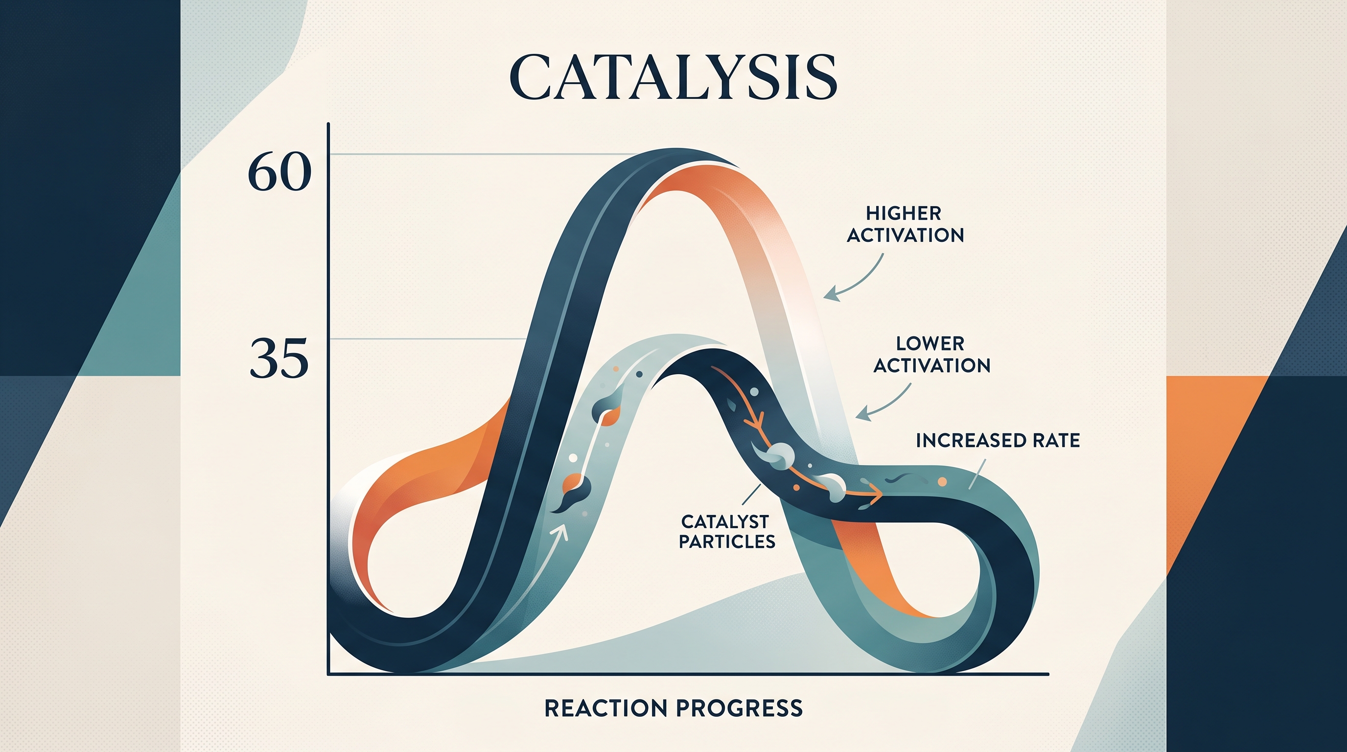
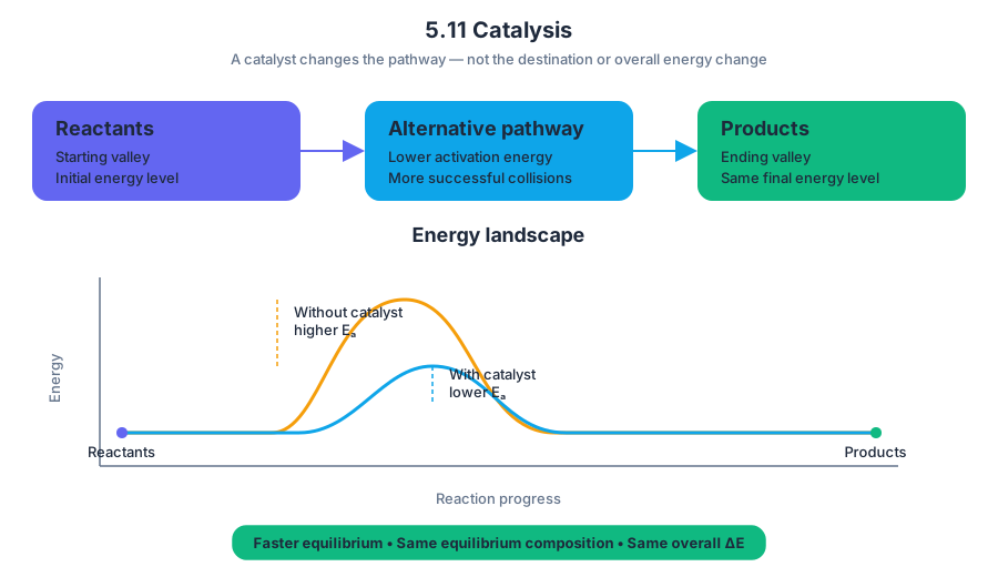
6.1 Endothermic and Exothermic Processes · 6.2 Energy Diagrams
Key concepts: Endothermic processes · Exothermic processes · Energy changes in a system · Energy transfer between a system and its surroundings · Heating and cooling of substances · Phase changes · Chemical transformations and reactions · Energy changes during bond formation · Dissolution and solution formation · Energy diagrams for physical and chemical transformations
A hand warmer becomes hot because its reacting system loses energy to its surroundings; an instant cold pack becomes cold because its dissolving system gains energy from its surroundings.
6.1 Endothermic and Exothermic Processes · 6.2 Energy Diagrams
A hand warmer becomes hot because its reacting system loses energy to its surroundings; an instant cold pack becomes cold because its dissolving system gains energy from its surroundings. The key question is not simply “Did the temperature change?” but which way did energy move, and what happened to the energy of the system?
System, surroundings, and energy change
The system is the chemical reaction or physical process being studied. Everything outside it—the water, container, air, and laboratory equipment—is the surroundings. Energy can cross the boundary between them through heat transfer or work.
Exothermic process: A process in which the energy of the system decreases and energy is released to the surroundings.
Endothermic process: A process in which the energy of the system increases because energy is transferred from the surroundings to the system.
For an exothermic process, the system loses energy and the surroundings gain it. For an endothermic process, the system gains energy and the surroundings lose it. A process may also have no net energy change when energy transfers balance overall; that does not mean that no energy was transferred.
Temperature changes provide observable evidence of energy changes, as required by 6.1.A.1. If a substance remains in the same phase and comparable conditions apply, a temperature increase usually indicates that the substance gained thermal energy, while a temperature decrease indicates that it lost thermal energy. During a phase change, however, energy can be redistributed without changing temperature, so temperature alone is not a complete measure of the system’s total energy.
Chemical and physical processes
6.1.A — Learning Objective: Explain the relationship between experimental observations and energy changes associated with a chemical or physical transformation.
6.1.A.2 identifies several types of energy-changing processes: heating or cooling a substance, phase changes, and chemical transformations. Each may be endothermic, exothermic, or have no net energy change.
Consider melting ice. The solid absorbs energy as water molecules overcome some of the attractions holding them in the crystal structure. The energy is endothermic, even if the ice-water mixture remains at a nearly constant temperature while melting occurs. By contrast, when liquid water freezes, the system releases energy to the surroundings: freezing is exothermic.
A chemical reaction follows the same system–surroundings logic. In combustion, bonds in the reactants must be broken, which requires energy. New bonds form in the products, releasing energy. The reaction is exothermic when the energy released by forming product bonds exceeds the energy required to break reactant bonds.
$$ \text{energy released during product-bond formation}
\text{energy required for reactant-bond breaking} $$
Dissolution: why a mixture can heat or cool
Dissolving a substance requires changes in intermolecular or interparticle attractions. Some attractions between solute particles and some attractions between solvent particles must be disrupted; new solute–solvent attractions then form. The formation of the solution may be exothermic or endothermic, depending on the relative thermal energies involved, as stated in 6.1.A.4.
Worked example — interpreting a dissolving experiment: A solid dissolves in water, and the temperature of the mixture falls from $24.0^\circ\mathrm{C}$ to $18.5^\circ\mathrm{C}$. The mixture became colder, so energy moved from the surroundings into the dissolving system. The dissolution is therefore endothermic.
If instead the mixture warmed from $24.0^\circ\mathrm{C}$ to $31.0^\circ\mathrm{C}$, the dissolving system would have released energy to the surroundings, making the dissolution exothermic.
Misconception check — “Dissolving always absorbs heat”: Dissolution is not automatically endothermic. Its energy change depends on the balance between attractions disrupted and attractions formed. A temperature decrease is evidence for endothermic dissolution; a temperature increase is evidence for exothermic dissolution, provided the measurement conditions are comparable.
Reading energy diagrams
An energy diagram represents the relative energy of a system before and after a chemical or physical transformation. The vertical axis should identify energy, often potential energy, with appropriate units; the horizontal axis should show reaction progress or the progress of the transformation. This use of labeled axes and scientifically appropriate representations develops Science Practice 3.A, Representing Data and Phenomena.
For an exothermic transformation, the products lie at a lower energy than the reactants:
$$ E_{\text{products}} < E_{\text{reactants}} $$
Thus, the system’s energy decreases and the difference is transferred to the surroundings. For an endothermic transformation, the products lie at a higher energy:
The system has gained energy from the surroundings.
The same diagram logic applies to both combustion and phase changes. A combustion diagram places the products below the reactants because combustion is exothermic. A melting or boiling diagram places the final phase at higher energy than the initial phase because energy is required to separate particles against their attractions.
Argument from observations
Science Practice 6.D, Argumentation: Provide reasoning to justify a claim using chemical principles or laws, or using mathematical justification. A strong argument connects the observation, the claim, and the mechanism:
- Observation: The solution temperature decreases.
- Claim: The dissolution is endothermic.
- Reasoning: The dissolving system gained energy from the surroundings, producing the observed cooling.
Retrieval check: A reaction mixture becomes warmer, while the chemical system is the process being studied. Is the reaction endothermic or exothermic? On an energy diagram, should the products appear above or below the reactants? The answer is exothermic: energy moved into the surroundings, so the products appear at lower energy than the reactants.
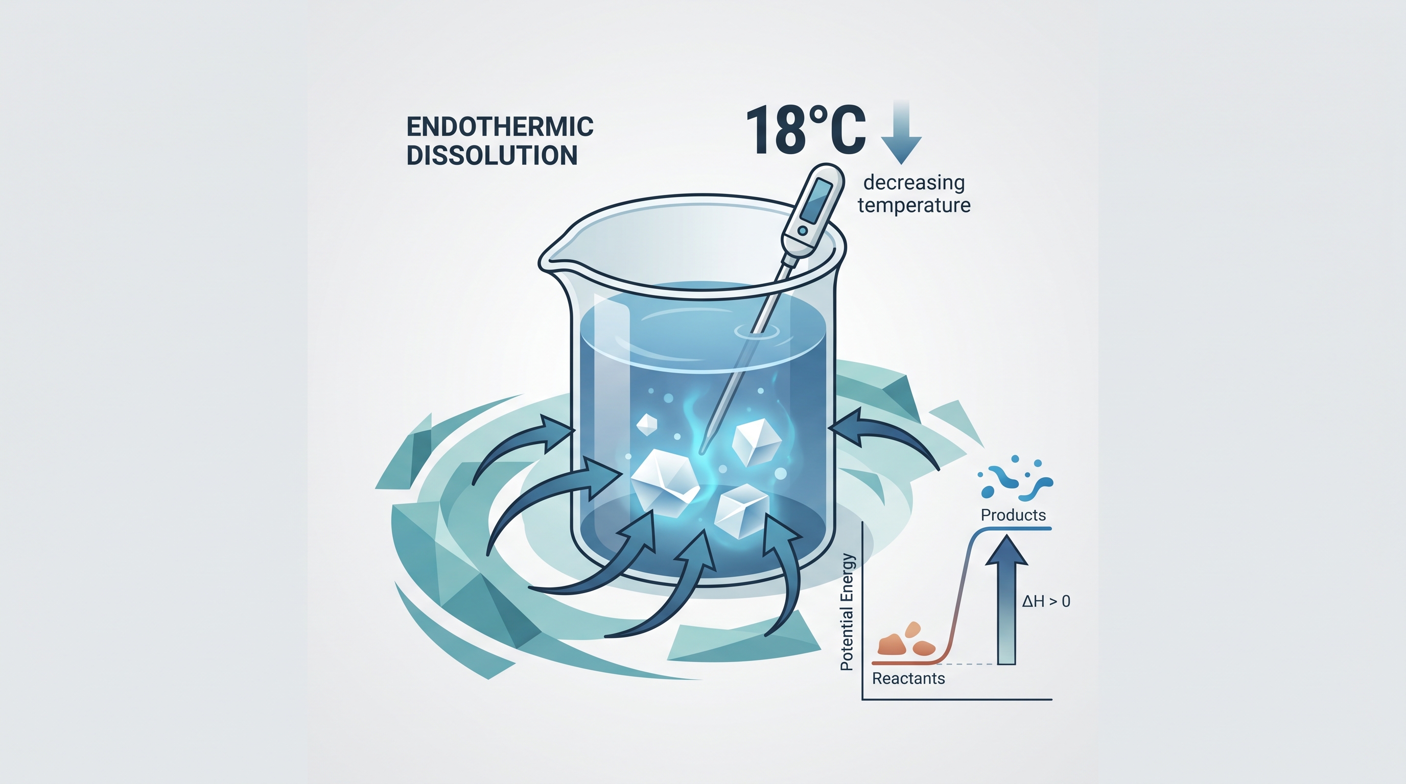
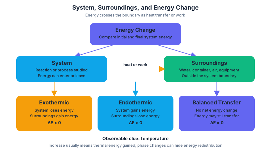
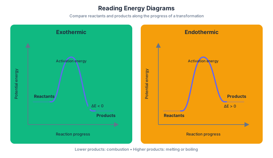
6.3 Heat Transfer and Thermal Equilibrium · 6.4 Heat Capacity and Calorimetry
Key concepts: Heat transfer between bodies in thermal contact · Thermal equilibrium · Particle collisions and transfer of thermal energy · Average kinetic energy and temperature · Specific heat capacity · Heat capacity · The heat-transfer equation · Calorimetry and energy conservation · Temperature change dependence on mass · Units of specific heat capacity
When a hot metal cube is dropped into cooler water, the metal cools while the water warms because microscopic collisions transfer thermal energy from faster-moving particles to slower-moving particles.
6.3 Heat Transfer and Thermal Equilibrium · 6.4 Heat Capacity and Calorimetry
When a hot metal cube is dropped into cooler water, the metal cools while the water warms because microscopic collisions transfer thermal energy from faster-moving particles to slower-moving particles.
Thermal energy moves through collisions
The particles in a warmer body have a greater average kinetic energy, meaning their particles move, vibrate, or rotate more energetically on average, than particles in a cooler body. When the two bodies are in thermal contact, particles at their boundary collide and redistribute energy.
The energy transfer is not caused by “cold moving” into the warmer object. Thermal energy is transferred as heat from the warmer body to the cooler body until both bodies have the same average kinetic energy and therefore the same temperature.
6.3.A.1: The particles in a warmer body have a greater average kinetic energy than those in a cooler body.
6.3.A.2: Collisions between particles in thermal contact can result in the transfer of energy; this is called heat transfer, heat exchange, or transfer of energy as heat.
6.3.A.3: At thermal equilibrium, the average kinetic energy and temperature of both bodies are the same.
Misconception check — “Thermal equilibrium means equal amounts of energy.” Not necessarily. Two objects can reach the same temperature while containing very different total thermal energies because total energy depends on the quantity of matter and the substance’s heat capacity. Thermal equilibrium means equal temperature, not equal mass or equal stored energy.
Quantifying heating and cooling
The heat transferred during a temperature change can be calculated with the heat-transfer equation:
$$q=mc\Delta T$$
Here, $q$ is the heat absorbed or released, $m$ is the mass, $c$ is the specific heat capacity, and $\Delta T$ is the temperature change:
$$\Delta T=T_{\text{final}}-T_{\text{initial}}$$
Specific heat capacity measures how much energy is required to change the temperature of one unit of mass by one degree. A common unit is $\mathrm{J/(g\cdot{}^\circ C)}$. Aluminum, for example, has a specific heat capacity of approximately:
$$c_{\text{Al}}=0.90\ \mathrm{J/(g\cdot{}^\circ C)}$$
For a fixed mass and temperature change, a larger $c$ requires more heat. Conversely, if equal masses receive the same amount of thermal energy, the substance with the smaller specific heat capacity undergoes the larger temperature change.
| Substance receiving the same heat | Relative specific heat capacity | Temperature change |
|---|---|---|
| Lower-$c$ substance | Smaller | Larger |
| Higher-$c$ substance | Larger | Smaller |
Worked comparison. Suppose $100\ \mathrm{g}$ of aluminum receives $900\ \mathrm{J}$:
$$\Delta T=\frac{q}{mc}=\frac{900\ \mathrm{J}}{(100\ \mathrm{g})(0.90\ \mathrm{J/(g\cdot{}^\circ C)})}=10.0^\circ\mathrm{C}$$
The same $900\ \mathrm{J}$ transferred to $100\ \mathrm{g}$ of water, with $c=4.18\ \mathrm{J/(g\cdot{}^\circ C)}$, produces:
$$\Delta T=\frac{900\ \mathrm{J}}{(100\ \mathrm{g})(4.18\ \mathrm{J/(g\cdot{}^\circ C)})}=2.15^\circ\mathrm{C}$$
The aluminum changes temperature more because each gram of aluminum requires less energy per degree.
Heat capacity and energy conservation
Heat capacity, represented by $C$, is the amount of heat needed to change the temperature of an entire object by one degree. Unlike specific heat capacity, which is intensive and independent of sample size, heat capacity depends on how much substance is present:
$$q=C\Delta T$$
Because $C=mc$, the two equations are equivalent:
$$q=mc\Delta T=C\Delta T$$
The first law of thermodynamics states that energy is conserved. In an insulated calorimetry experiment, heat lost by one body is gained by another:
$$q_{\text{hot}}+q_{\text{cold}}=0$$
A positive $q$ indicates that a body absorbs heat; a negative $q$ indicates that it releases heat. Heating increases a system’s energy, while cooling decreases it.
Calorimetry: measuring an unknown heat capacity
Calorimetry determines heat transfer by tracking temperature changes, usually while limiting heat exchange with the surroundings. A hot metal placed in cooler water provides a direct application: calculate the water’s heat gain, set it equal in magnitude to the metal’s heat loss, and solve for the metal’s specific heat.
Worked calorimetry example. A $98.1\ \mathrm{g}$ metal sample cools from $100.0^\circ\mathrm{C}$ to $38.5^\circ\mathrm{C}$ and releases $2940\ \mathrm{J}$. Thus:
$$q_{\text{metal}}=-2940\ \mathrm{J}$$
$$\Delta T_{\text{metal}}=38.5^\circ\mathrm{C}-100.0^\circ\mathrm{C}=-61.5^\circ\mathrm{C}$$
Solving $q=mc\Delta T$ for the unknown specific heat gives:
$$c_{\text{metal}}=\frac{q_{\text{metal}}}{m_{\text{metal}}\Delta T_{\text{metal}}} =\frac{-2940\ \mathrm{J}}{(98.1\ \mathrm{g})(-61.5^\circ\mathrm{C})} =0.487\ \mathrm{J/(g\cdot{}^\circ C)}$$
The two negative signs are important: the metal releases heat and its temperature decreases. Their ratio produces the positive specific heat capacity expected for a substance.
AP reasoning in action
This topic uses Science Practice 1: Models and Representations when particle arrows represent average kinetic energy, Science Practice 3: Representing Data and Phenomena when a temperature change is connected to a microscopic collision model, and Science Practice 5: Mathematical Routines when $q=mc\Delta T$ and energy conservation are applied. A strong explanation connects all three: the hot sample’s particles collide with cooler-water particles, transfer energy, and produce the measured temperature changes.
Retrieval check. Two equal-mass samples absorb the same heat. Sample A has a smaller specific heat capacity than Sample B. Which sample has the larger $\Delta T$, and why? The correct reasoning is that Sample A has the larger temperature change because $\Delta T=q/(mc)$ and its smaller $c$ makes the denominator smaller.
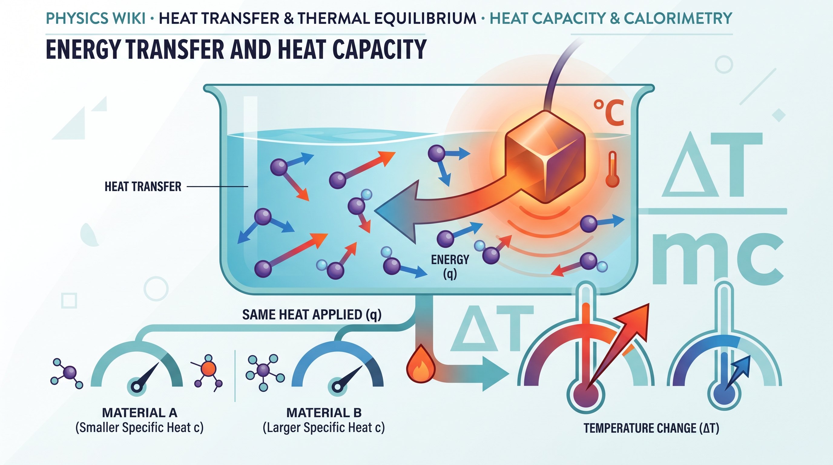
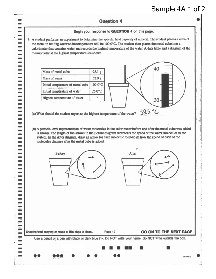
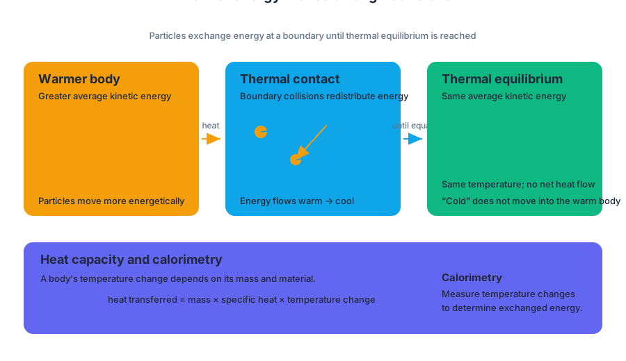
6.5 Energy of Phase Changes · 6.6 Introduction to Enthalpy of Reaction
Key concepts: Energy changes during phase changes · Constant temperature during a phase change · Enthalpy relationships for opposite phase changes · Heat and amount of reacting substance · Enthalpy of reaction at constant pressure · Multi-step thermochemical calculations with units and significant figures
A pure substance can absorb or release energy during a phase change without changing temperature because the energy changes particle arrangement rather than average kinetic energy.
6.5 Energy of Phase Changes · 6.6 Introduction to Enthalpy of Reaction
A pure substance can absorb or release energy during a phase change without changing temperature because the energy changes particle arrangement rather than average kinetic energy. Melting and vaporization require energy input; freezing and condensation release energy.
6.5 Energy of Phase Changes
Learning Objective 6.5.A: Explain changes in the heat $q$ absorbed or released by a system undergoing a phase transition based on the amount of substance in moles and the molar enthalpy of the phase transition.
Essential Knowledge 6.5.A.1: Energy must be transferred to a system for melting or boiling. During these processes, particles move into a higher-energy arrangement. During freezing or condensing, the system releases energy as particles move into a lower-energy arrangement.
During a phase change, the temperature of a pure substance remains constant. On a heating curve, this appears as a horizontal segment: energy continues entering the system, but the temperature does not rise. The incoming energy is being used to overcome intermolecular attractions or reorganize particles, not to increase their average kinetic energy.
The heat transferred is calculated from the amount of substance and the molar enthalpy of the phase transition:
$$q=n\Delta H_{\text{phase}}$$
where $q$ is heat in $\text{kJ}$ or $\text{J}$, $n$ is the amount in $\text{mol}$, and $\Delta H_{\text{phase}}$ is the molar enthalpy in $\text{kJ mol}^{-1}$ or $\text{J mol}^{-1}$.
Opposite phase changes
Essential Knowledge 6.5.A.2: The energy absorbed in one direction equals the energy released in the reverse direction with the opposite sign. For vaporization and condensation,
$$\Delta H_{\text{cond}}=-\Delta H_{\text{vap}}$$
Similarly, melting has a positive enthalpy, while freezing has the corresponding negative enthalpy:
$$\Delta H_{\text{freezing}}=-\Delta H_{\text{fusion}}$$
Worked example — vaporization and condensation: Suppose $\Delta H_{\text{vap}}$ for water is $40.7\ \text{kJ mol}^{-1}$. Vaporizing $2.00\ \text{mol}$ requires
$$q=(2.00\ \text{mol})\left(40.7\ \frac{\text{kJ}}{\text{mol}}\right)=81.4\ \text{kJ}$$
The reverse process releases the same magnitude:
$$q_{\text{cond}}=(2.00\ \text{mol})\left(-40.7\ \frac{\text{kJ}}{\text{mol}}\right)=-81.4\ \text{kJ}$$
The negative sign identifies energy leaving the condensing system.
Misconception check — “Temperature always rises when energy is added.” Not during a phase change of a pure substance. A temperature increase indicates increasing average kinetic energy; the flat portion of a heating curve represents energy changing particle attractions and spacing instead.
6.6 Introduction to Enthalpy of Reaction
Most AP-level reactions are studied at constant pressure. Under these conditions, the system’s enthalpy change, $\Delta H_{\text{rxn}}$, corresponds to the heat transferred at constant pressure:
$$q_p=\Delta H_{\text{rxn}}$$
For a reaction amount measured in moles,
$$q=n\Delta H_{\text{rxn}}$$
A negative $\Delta H_{\text{rxn}}$ indicates an exothermic reaction; a positive value indicates an endothermic reaction.
The amount $n$ must refer to the reaction quantity specified by the balanced chemical equation. If twice as much reacting substance reacts, twice as much total heat is transferred, but the molar enthalpy remains unchanged.
Worked example — reaction heat: A reaction has $\Delta H_{\text{rxn}}=-450\ \text{kJ mol}{\text{rxn}}^{-1}$. If $0.0500\ \text{mol}{\text{rxn}}$ occurs,
$$q_{\text{rxn}}=(0.0500\ \text{mol}{\text{rxn}}) \left(-450\ \frac{\text{kJ}}{\text{mol}{\text{rxn}}}\right) =-22.5\ \text{kJ}$$
The reaction releases $22.5\ \text{kJ}$, so the surroundings absorb approximately $22.5\ \text{kJ}$.
If the reacting amount is given as a mass, convert it to moles before using $q=n\Delta H$. For example, if $5.00\ \text{g}$ of a substance with molar mass $100.0\ \text{g mol}^{-1}$ reacts,
$$n=5.00\ \text{g}\left(\frac{1\ \text{mol}}{100.0\ \text{g}}\right)=0.0500\ \text{mol}$$
Then substitute this amount into the enthalpy relationship. Dimensional analysis should leave heat units, and the final answer should match the least precise measured quantity in significant figures.
AP skills and representations
Suggested Skill 1.B — Models and Representations: Describe components and quantitative information in models that connect particulate-level and macroscopic properties. Here, a heating curve or particle diagram should be interpreted together with $q$, $n$, and $\Delta H$: a flat temperature region represents a microscopic rearrangement while the equation reports its macroscopic energy cost.
Suggested Skill 5.F — Model Analysis: Perform multi-step calculations while tracking units and significant figures. A strong response shows the conversion from mass to moles, the enthalpy relationship, the sign convention, and a correctly rounded result.
Misconception check — “A negative heat means the surroundings lose energy.” The sign belongs to the system whose heat is being reported. For an exothermic reaction, $q_{\text{rxn}}<0$, while the surroundings gain energy. Confusing $q_{\text{rxn}}$ with $q_{\text{surroundings}}$ reverses the conclusion.
Retrieval check: A sample undergoes condensation with $\Delta H_{\text{vap}}=35.0\ \text{kJ mol}^{-1}$. What is $q$ when $0.250\ \text{mol}$ condenses? The correct setup is $q=(0.250\ \text{mol})(-35.0\ \text{kJ mol}^{-1})=-8.75\ \text{kJ}$: energy is released, and the temperature remains constant during the phase change.
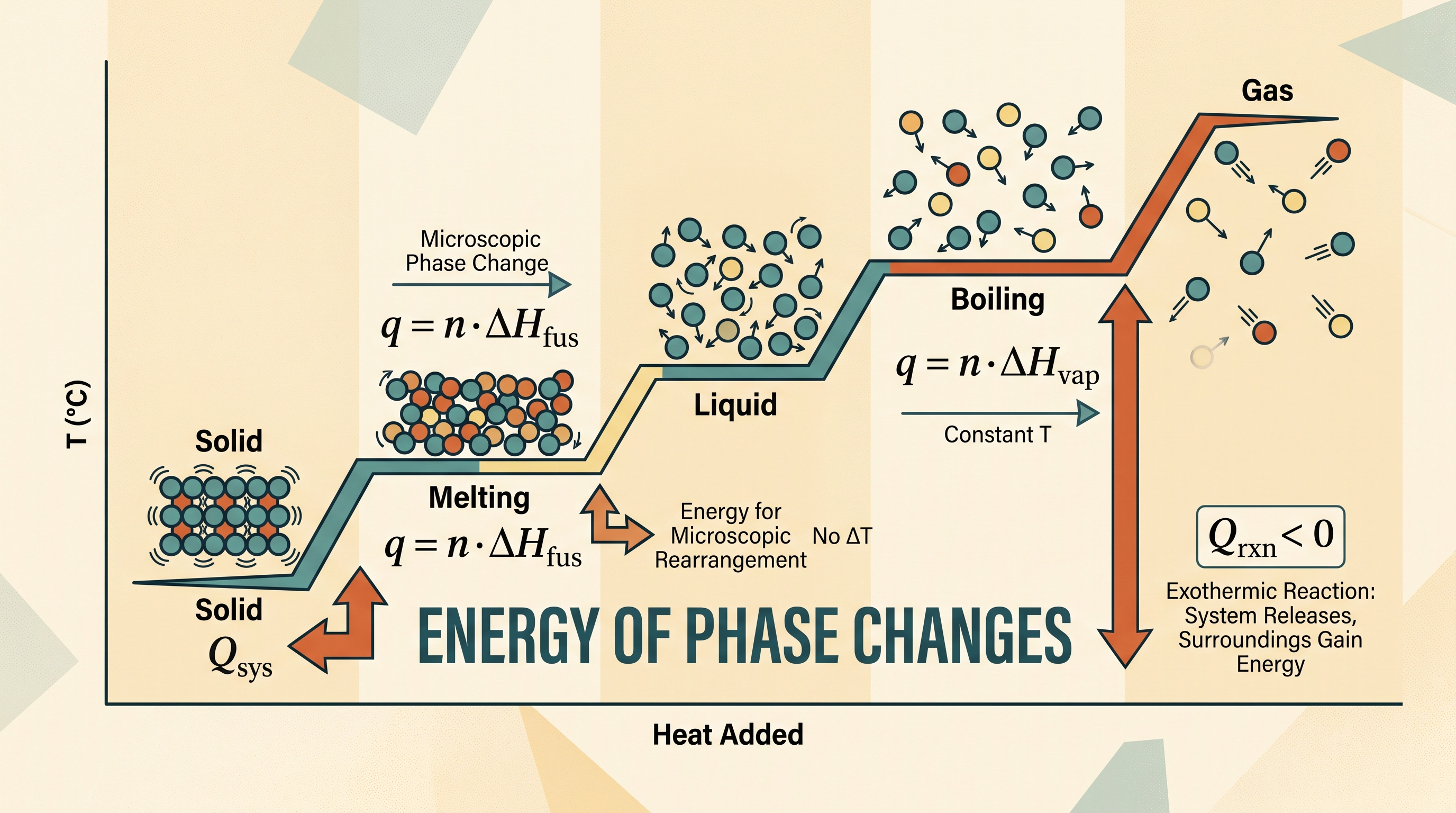
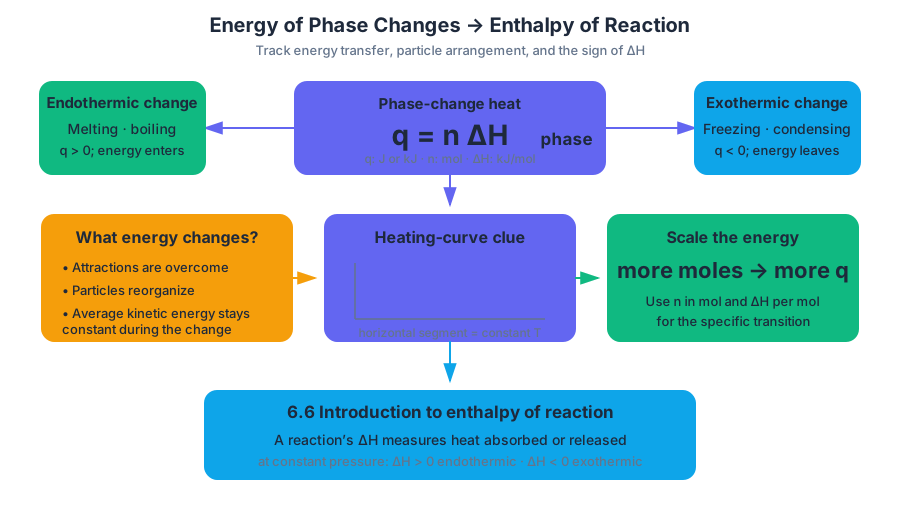
6.7 Bond Enthalpies · 6.8 Enthalpy of Formation
Key concepts: Bond enthalpy and the relationship between bond formation and energy · Standard enthalpy of formation (ΔH°f) · Hess’s law and manipulating formation reactions · Calculating an unknown quantity from known quantities using a logical computational pathway · Standard states and elemental reference values · Enthalpy change for synthesizing a compound from its elements · Sign conventions for energy released and absorbed · Dimensional analysis and significant figures in thermochemical calculations · Lattice enthalpy data for ionic compounds · Using tables of standard enthalpies of formation
A chemical bond forms when atomic orbitals overlap and the resulting attraction lowers the system’s potential energy; breaking that bond requires energy, while forming it releases energy.
6.7 Bond Enthalpies · 6.8 Enthalpy of Formation
A chemical bond forms when atomic orbitals overlap and the resulting attraction lowers the system’s potential energy; breaking that bond requires energy, while forming it releases energy. These two opposite energy changes connect molecular structure to reaction enthalpy.
Bond enthalpies: an energy estimate from bonds
A bond enthalpy is the energy required to break one mole of a particular bond in gaseous molecules. Because the same type of bond can exist in slightly different molecular environments, tabulated bond enthalpies are average values, so calculations based on them estimate rather than exactly determine $\Delta H^\circ_{\mathrm{rxn}}$.
For a reaction, count the bonds broken in reactants and the bonds formed in products:
$$ \Delta H_{\mathrm{rxn}} \approx \sum E(\text{bonds broken})
\sum E(\text{bonds formed}) $$
The subtraction reflects the energy direction: breaking bonds consumes energy and forming bonds releases energy. If the newly formed bonds release more energy than the reactant bonds required to break, the reaction is exothermic and $\Delta H_{\mathrm{rxn}}<0$.
Worked pathway: estimating a reaction enthalpy
Suppose a gaseous reaction breaks two bonds with enthalpies $400.\ \mathrm{kJ,mol^{-1}}$ and $500.\ \mathrm{kJ,mol^{-1}}$, then forms three bonds with enthalpies $300.\ \mathrm{kJ,mol^{-1}}$ each:
$$ \Delta H_{\mathrm{rxn}} \approx (400.+500.)- 3(300.) $$
$$ \Delta H_{\mathrm{rxn}} \approx 900.-900.
0.\ \mathrm{kJ,mol^{-1}_{rxn}} $$
The explicit decimal points communicate that $400.$ and $500.$ are measured to the ones place, not ambiguous values with unknown precision. Bond-enthalpy estimates are especially useful for comparing reactions, but a standard enthalpy of formation or calorimetric value is preferred when an exact tabulated value is available. Molecular orbital theory is not a recommended deeper method for explaining multiple bonds here; the required reasoning is based on bond energies and orbital overlap.
Misconception check: A strong bond does not release energy when it is broken. Bond breaking always requires energy; bond formation releases energy because the bonded arrangement is lower in potential energy.
Standard enthalpy of formation
The standard enthalpy of formation, $\Delta H_f^\circ$, is the enthalpy change for forming exactly one mole of a compound from its constituent elements in their specified standard states. The standard state is the reference form of a substance at a specified standard pressure, commonly $1\ \mathrm{bar}$, and a stated temperature, commonly $298.15\ \mathrm{K}$; therefore, a quoted $\Delta H_f^\circ$ is tied to that temperature.
Every element in its standard state has $\Delta H_f^\circ=0\ \mathrm{kJ,mol^{-1}}$. Relevant reference forms include $\mathrm{Na(s)}$, $\frac{1}{2}\mathrm{O_2(g)}$, $\frac{1}{4}\mathrm{P_4(s)}$, and $\frac{3}{2}\mathrm{Cl_2(g)}$. The fractional coefficients are necessary when the formation reaction produces exactly one mole of compound.
| Substance in standard state | $\Delta H_f^\circ$ |
|---|---|
| $\mathrm{Na(s)}$ | $0\ \mathrm{kJ,mol^{-1}}$ |
| $\mathrm{O_2(g)}$ | $0\ \mathrm{kJ,mol^{-1}}$ |
| $\mathrm{P_4(s)}$ | $0\ \mathrm{kJ,mol^{-1}}$ |
| $\mathrm{Cl_2(g)}$ | $0\ \mathrm{kJ,mol^{-1}}$ |
Worked example: forming $\mathrm{Na_2O(s)}$
The synthesis reaction is
$$ 2\mathrm{Na(s)}+\frac{1}{2}\mathrm{O_2(g)} \rightarrow \mathrm{Na_2O(s)} $$
with
$$ \Delta H^\circ_{\mathrm{rxn}}
-828\ \mathrm{kJ,mol^{-1}_{rxn}} $$
Because the reactants are elements in their standard states,
$$ \Delta H^\circ_{\mathrm{rxn}}
\Delta H_f^\circ[\mathrm{Na_2O(s)}]
\left[ 2\Delta H_f^\circ[\mathrm{Na(s)}] + \frac{1}{2}\Delta H_f^\circ[\mathrm{O_2(g)}] \right] $$
$$ -828
\Delta H_f^\circ[\mathrm{Na_2O(s)}]
[2(0)+\tfrac{1}{2}(0)] $$
$$ \boxed{\Delta H_f^\circ[\mathrm{Na_2O(s)}]
-828\ \mathrm{kJ,mol^{-1}}} $$
The unit $\mathrm{kJ,mol^{-1}_{rxn}}$ means $828\ \mathrm{kJ}$ is released per mole of reaction as written—not per mole of sodium atoms or per mole of oxygen molecules.
Manipulating formation reactions
Known formation reactions can be combined through Hess’s law. Reverse a reaction and change the sign of $\Delta H$; multiply every coefficient by a factor and multiply $\Delta H$ by that same factor. The intermediate species must cancel when the equations are added.
For phosphorus pentachloride, first scale the phosphorus trichloride formation reaction:
$$ \frac14\mathrm{P_4(s)}+\frac32\mathrm{Cl_2(g)} \rightarrow \mathrm{PCl_3(g)} \qquad \Delta H_1^\circ=-287\ \mathrm{kJ,mol^{-1}_{rxn}} $$
Then add
$$ \mathrm{PCl_3(g)}+\mathrm{Cl_2(g)} \rightarrow \mathrm{PCl_5(g)} \qquad \Delta H_2^\circ=-88\ \mathrm{kJ,mol^{-1}_{rxn}} $$
Cancel $\mathrm{PCl_3(g)}$:
$$ \frac14\mathrm{P_4(s)}+\frac52\mathrm{Cl_2(g)} \rightarrow \mathrm{PCl_5(g)} $$
$$ \Delta H_f^\circ[\mathrm{PCl_5(g)}]
-287+(-88)
\boxed{-375\ \mathrm{kJ,mol^{-1}}} $$
Precision rule: Carry units and guard digits through intermediate steps. For addition or subtraction, round according to decimal places; for multiplication or division, round according to significant figures. Round the final result only to the precision justified by the given data.
AP Skill 5.F — “Calculate, estimate, or predict an unknown quantity from known quantities by selecting and following a logical computational pathway and attending to precision.” Show the reaction manipulation, cancellation, units, and final precision—not merely the numerical answer.
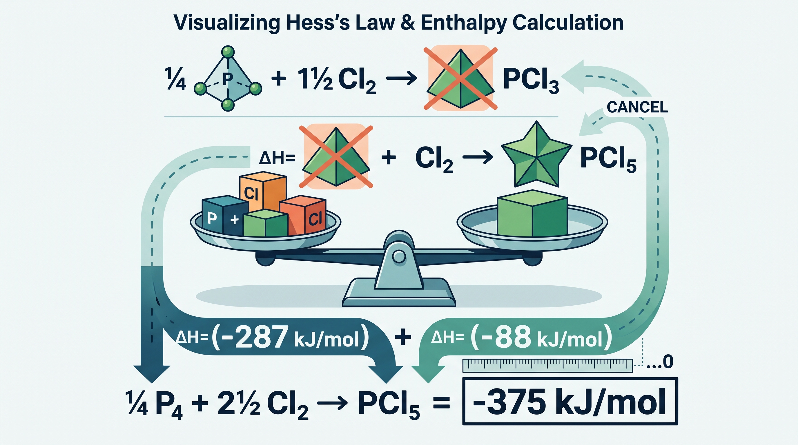
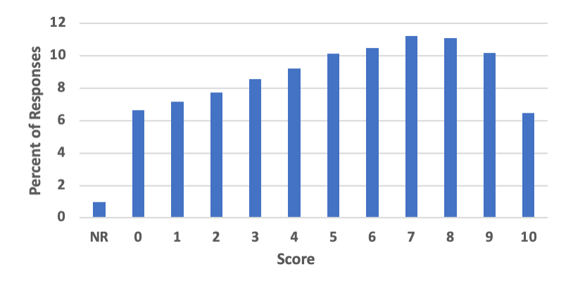
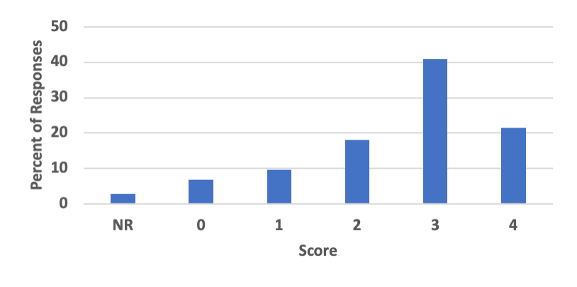
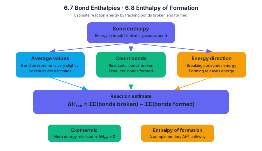
6.9 Hess’s Law
Key concepts: Hess’s law · Enthalpy of formation · Adding enthalpy-change values · Manipulating thermochemical equations · Using tabulated data · Molecular mass of Cl(g)
A reaction’s enthalpy change depends only on the starting substances and final substances, not on the route taken between them. Hess’s law turns that fact into a calculation method: if a target reaction can be built by adding known thermochemical equations, its overall enthalpy change is the sum of the…
6.9 Hess’s Law
A reaction’s enthalpy change depends only on the starting substances and final substances, not on the route taken between them. Hess’s law turns that fact into a calculation method: if a target reaction can be built by adding known thermochemical equations, its overall enthalpy change is the sum of the appropriately manipulated $\Delta H$ values.
Hess’s law: When chemical equations are added, their enthalpy changes are added as well—provided every equation is first adjusted so that the chemical species and coefficients combine to give the desired overall reaction.
The equation-manipulation rule
Thermochemical equations behave like algebraic equations, but their $\Delta H$ values must be manipulated at the same time.
- Reverse an equation: reverse the sign of $\Delta H$.
- Multiply every coefficient by a factor: multiply $\Delta H$ by the same factor.
- Add equations: cancel species appearing on opposite sides, then add the adjusted $\Delta H$ values.
- Do not alter $\Delta H$ merely because a species is written on a different side after cancellation; the sign changes only when the entire reaction is reversed.
Worked example: building a target reaction
Suppose the target reaction is the formation of methane from its elements:
$$ \mathrm{C(s) + 2H_2(g) \rightarrow CH_4(g)} $$
The available thermochemical equations are:
$$ \mathrm{C(s) + O_2(g) \rightarrow CO_2(g)} \qquad \Delta H_1^\circ=-393.5\ \mathrm{kJ,mol^{-1}} $$
$$ \mathrm{H_2(g) + \frac{1}{2}O_2(g) \rightarrow H_2O(l)} \qquad \Delta H_2^\circ=-285.8\ \mathrm{kJ,mol^{-1}} $$
$$ \mathrm{CH_4(g) + 2O_2(g) \rightarrow CO_2(g) + 2H_2O(l)} \qquad \Delta H_3^\circ=-890.3\ \mathrm{kJ,mol^{-1}} $$
The target contains $2\mathrm{H_2}$, so multiply the second equation by $2$:
$$ \mathrm{2H_2(g) + O_2(g) \rightarrow 2H_2O(l)} $$
$$ \Delta H_2' = 2(-285.8)=-571.6\ \mathrm{kJ,mol^{-1}} $$
The target has $\mathrm{CH_4}$ as a product, but equation $3$ has $\mathrm{CH_4}$ as a reactant. Reverse equation $3$ and change the sign of its enthalpy:
$$ \mathrm{CO_2(g) + 2H_2O(l) \rightarrow CH_4(g) + 2O_2(g)} $$
$$ \Delta H_3'=+890.3\ \mathrm{kJ,mol^{-1}} $$
Now add the three adjusted equations:
$$ \begin{aligned} \mathrm{C(s)+O_2(g)} &\rightarrow \mathrm{CO_2(g)} \ \mathrm{2H_2(g)+O_2(g)} &\rightarrow \mathrm{2H_2O(l)} \ \mathrm{CO_2(g)+2H_2O(l)} &\rightarrow \mathrm{CH_4(g)+2O_2(g)} \end{aligned} $$
Cancel $\mathrm{CO_2}$ and $\mathrm{2H_2O}$ because each appears on both sides. Cancel the two $\mathrm{O_2}$ molecules on the reactant side against the two on the product side. The result is exactly the target reaction:
Finally, add the adjusted enthalpy values:
$$ \Delta H^\circ
(-393.5)+(-571.6)+(+890.3)
-74.8\ \mathrm{kJ,mol^{-1}} $$
The negative value means that forming $1\ \mathrm{mol}$ of $\mathrm{CH_4(g)}$ from the elements, under the stated conditions, is exothermic.
Using tabulated enthalpy data
A table may provide standard enthalpy changes for reactions, including standard enthalpies of formation, $\Delta H_f^\circ$. The table values are not automatically ready to add. First compare each tabulated equation with the target: reverse, scale, or leave it unchanged as required. Only then combine the numbers.
A common scoring error is to reverse a chemical equation but keep the original sign. Another is to multiply coefficients—such as changing $1\mathrm{mol}$ of a substance to $2\mathrm{mol}$—without multiplying $\Delta H$. Both errors produce a chemically inconsistent result even if the final arithmetic is flawless.
Do not confuse enthalpy with concentration
Hess’s-law calculations use reaction equations and energy changes, not concentration values. A concentration may appear in the surrounding experimental information, but it belongs in a different calculation unless the question explicitly asks you to convert an amount into moles or determine a reaction quantity.
The same distinction applies to elemental chlorine. The atomic species $\mathrm{Cl(g)}$ has molecular mass approximately
$$ M_{\mathrm{Cl(g)}}=35.45\ \mathrm{g,mol^{-1}} $$
whereas molecular chlorine, $\mathrm{Cl_2(g)}$, has molar mass
$$ M_{\mathrm{Cl_2(g)}}=70.90\ \mathrm{g,mol^{-1}} $$
Thus, if a calculation involves $7.09\ \mathrm{g}$ of $\mathrm{Cl(g)}$:
$$ n=\frac{7.09\ \mathrm{g}}{35.45\ \mathrm{g,mol^{-1}}}=0.200\ \mathrm{mol} $$
Using $70.90\ \mathrm{g,mol^{-1}}$ would incorrectly treat chlorine atoms as $\mathrm{Cl_2}$ molecules.
AP skill connection and retrieval check
This problem pattern develops Science Practice 1: Models and Representations, because equations model chemical processes; Science Practice 4: Model Analysis, because you inspect and transform those models; and Science Practice 5: Mathematical Routines, because you scale and add enthalpy values. A strong written response also uses Science Practice 6: Argumentation when it explains why cancellation produces the target reaction.
Retrieval check: If a supplied equation is multiplied by $\frac{3}{2}$ and has $\Delta H= -40\ \mathrm{kJ,mol^{-1}}$, what enthalpy belongs to the adjusted equation? If the equation is also reversed, what is the final value?
Answer: scaling gives
$$ \Delta H=\frac{3}{2}(-40)=-60\ \mathrm{kJ,mol^{-1}} $$
Reversing the scaled equation changes the sign, so the final value is
$$ \boxed{+60\ \mathrm{kJ,mol^{-1}}} $$
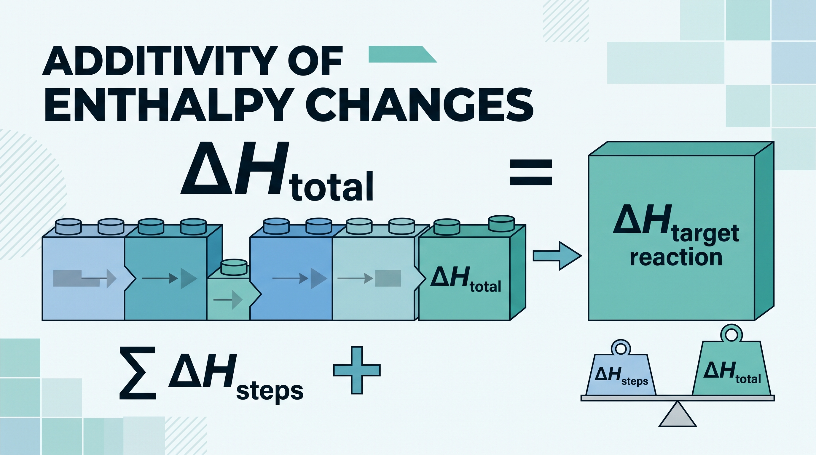
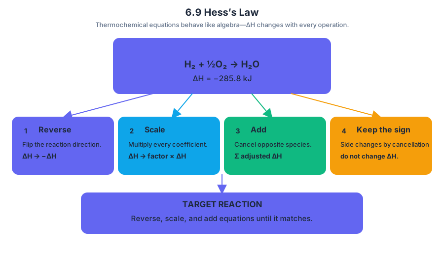
7.1 Introduction to Equilibrium · 7.2 Direction of Reversible Reactions
Key concepts: Equilibrium · Introduction to equilibrium · Direction of reversible reactions · Le Châtelier’s principle · Particulate representations of equilibrium systems · Model analysis · Required course content for AP Chemistry Unit 7
A reversible reaction does not simply “run forward until the reactants disappear.” In a closed system, products can react to reform reactants while reactants continue forming products.
7.1 Introduction to Equilibrium · 7.2 Direction of Reversible Reactions
A reversible reaction does not simply “run forward until the reactants disappear.” In a closed system, products can react to reform reactants while reactants continue forming products. Equilibrium is the dynamic state in which the forward and reverse reactions occur at equal rates, so the macroscopic composition remains constant even though particles continue reacting.
Unit 7, Equilibrium, represents approximately $7$–$9%$ of the AP Chemistry Exam. The central question is not whether a reaction stops, but how the relative rates of opposing reactions determine the system’s direction and response to change.
Reversible reactions: two directions at once
A reversible reaction is represented with opposing arrows:
$$ \text{reactants} \rightleftharpoons \text{products} $$
Imagine a crowded doorway connecting two rooms. At first, many people move from Room A into Room B, so the population of Room B rises quickly. As Room B becomes more crowded, more people begin returning to Room A. Eventually, people still pass through the doorway in both directions, but the number moving each way per unit time is equal. The populations remain steady even though motion continues.
The same logic applies chemically. Topic 7.2 Direction of Reversible Reactions focuses on how the relative rates of the forward and reverse reactions determine the net direction of change.
Essential Knowledge 7.2.A.1: If the forward reaction is faster than the reverse reaction, there is a net conversion of reactants to products. If the reverse reaction is faster, there is a net conversion of products to reactants. Equilibrium is reached when the two rates are equal.
The changing direction of a reaction
Consider the reversible reaction
A \rightleftharpoons B
Immediately after placing mostly $A$ in the container, the forward rate is relatively large because many $A$ particles can collide and convert into $B$. The reverse rate is initially small because few $B$ particles are present. Therefore, the system undergoes a net conversion of $A$ to $B$.
As $A$ is consumed, the forward rate tends to decrease. As $B$ accumulates, the reverse rate tends to increase. The system reaches equilibrium when
$$ \text{rate}{\text{forward}}=\text{rate}{\text{reverse}} $$
At equilibrium, the concentrations of $A$ and $B$ are constant, but they are not necessarily equal. Equal rates do not mean equal amounts of reactants and products.
Dynamic equilibrium means that opposing microscopic processes continue at equal rates while observable, macroscopic properties remain constant.
Particulate diagrams: seeing equilibrium at the particle level
A particulate diagram models a chemical system by drawing individual atoms, molecules, or ions. It can show whether a system contains only reactants, only products, or a stable mixture of both. The diagram is useful because equilibrium is invisible at the macroscopic level: a flask may appear unchanged while particles continue to transform.
To analyze a particulate representation, count species, not merely shapes. A species is a distinct chemical entity identified by its composition and charge. For example, in a diagram containing $4$ molecules of $A_2$, $3$ molecules of $B$, and $2$ molecules of $AB$, the total number of represented particles is
$$ 4+3+2=9\text{ particles} $$
However, the number of particles is not the same as the number of species types. That diagram contains three species types: $A_2$, $B$, and $AB$. Also distinguish molecules from atoms: one $A_2$ particle contains two atoms, whereas one $B$ particle contains one atom.
Misconception check — “Equilibrium means equal amounts.”
False. Equilibrium means equal forward and reverse rates. A system may contain mostly reactants, mostly products, or comparable amounts of both.
Le Châtelier’s principle: predicting a response
Le Châtelier’s principle predicts the qualitative response of an equilibrium system after a disturbance: when a system at equilibrium is changed, it shifts in the direction that tends to reduce the effect of that change and establish a new equilibrium.
For example, if additional reactant is added to
A \rightleftharpoons B
the system responds by favoring the direction that consumes some of the added $A$—the forward direction. If additional $B$ is added, the system favors the reverse direction, consuming some of the added product. The shift does not remove the disturbance completely; it reduces its effect while producing a new equilibrium composition.
This principle has a laboratory application in Investigation 13, “Can We Make the Colors of the Rainbow? An Application of Le Châtelier’s Principle.” Color changes provide a macroscopic signal that the particulate-level balance of an equilibrium system has changed.
AP Science Practice connection: Model Analysis
The suggested skill is 4.D — Model Analysis: Explain the degree to which a model or representation describes the connection between particulate-level properties and macroscopic properties. A strong explanation links the diagram to observable evidence: unequal forward and reverse rates produce a net composition change, while equal rates produce constant macroscopic composition.
A model is not the chemical system itself. A particulate drawing may omit solvent molecules, show only a sample of particles, or use symbols that are not to scale. Use it to identify trends and relationships, but count carefully and state what the representation actually supports.
Retrieval check
A sealed container initially contains many product particles and very few reactant particles. The reverse reaction is faster than the forward reaction. What happens first, and what condition eventually signals equilibrium?
Answer: There is a net conversion of products into reactants. As the relative rates change, the system approaches a state in which the forward and reverse rates are equal; particles continue reacting, but the macroscopic composition remains constant.
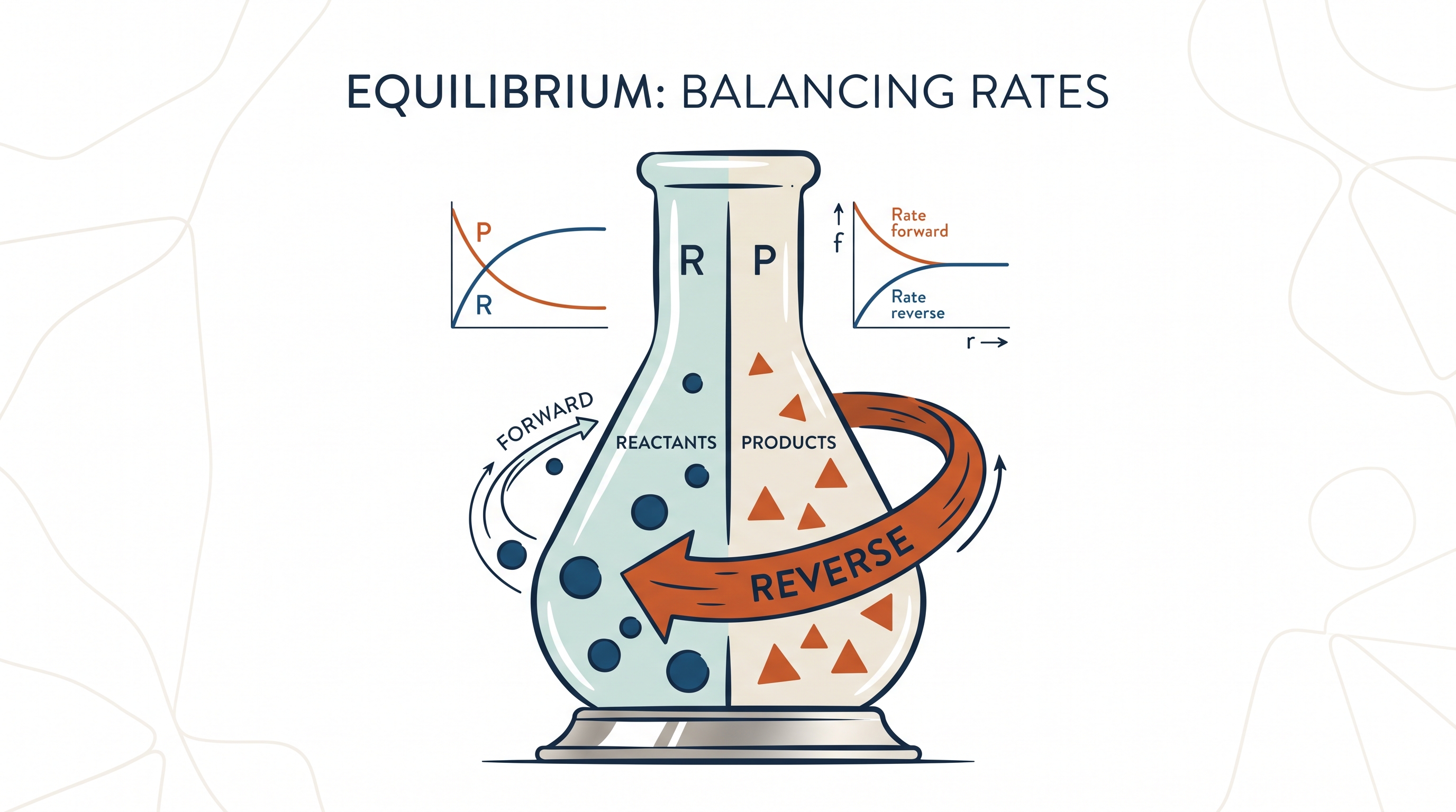
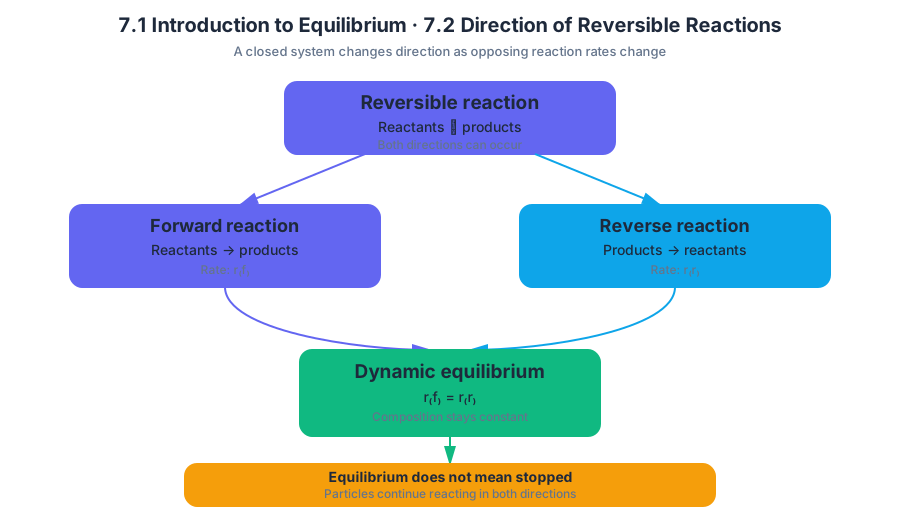
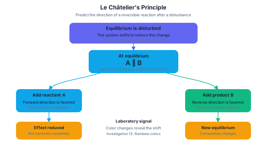
7.3 Reaction Quotient and Equilibrium Constant · 7.4 Calculating the Equilibrium Constant
Key concepts: Reaction quotient Qc · Reaction quotient Qp · Equilibrium constant Kc · Equilibrium constant Kp · Law of mass action · Equilibrium mixtures and reversible reactions · Equilibrium concentrations · Equilibrium partial pressures · Comparing Q with K to determine equilibrium status
A reversible reaction can be treated like a molecular tug-of-war: the mixture may begin with mostly reactants, mostly products, or something in between, but its composition can be measured at any instant.
7.3 Reaction Quotient and Equilibrium Constant · 7.4 Calculating the Equilibrium Constant
A reversible reaction can be treated like a molecular tug-of-war: the mixture may begin with mostly reactants, mostly products, or something in between, but its composition can be measured at any instant. The reaction quotient, $Q$, measures the mixture’s current product-to-reactant relationship; the equilibrium constant, $K$, is that same relationship specifically when the system has reached equilibrium.
From a reversible equation to an equilibrium expression
For the general reversible reaction
aA+bB\rightleftharpoons cC+dD
the lowercase letters are stoichiometric coefficients, and the uppercase letters represent chemical species. The law of mass action says that the reaction expression places product terms in the numerator, reactant terms in the denominator, and raises every concentration or pressure to the power of its coefficient.
Concentration form: $Q_c$ and $K_c$
The concentration reaction quotient, $Q_c$, describes the relative concentrations of reaction species at any point in time:
$$Q_c=\frac{[C]^c[D]^d}{[A]^a[B]^b}$$
Square brackets, such as $[A]$, represent concentration, usually molarity. If the mixture is at equilibrium, the measured concentrations produce the equilibrium constant:
$$Q_c=K_c$$
Before equilibrium, the same expression is called $Q_c$, not $K_c$.
Pressure form: $Q_p$ and $K_p$
For a gas-phase reaction, the expression may use partial pressures instead:
$$Q_p=\frac{(P_C)^c(P_D)^d}{(P_A)^a(P_B)^b}$$
Here, $P_A$, $P_B$, $P_C$, and $P_D$ are the partial pressures of the species. At equilibrium,
$$Q_p=K_p$$
The structure of the expression does not change; only the measured quantity changes from concentration to partial pressure.
| Quantity | What it describes | Values used | At equilibrium |
|---|---|---|---|
| $Q_c$ | Current composition of a mixture | Concentrations | $Q_c=K_c$ |
| $Q_p$ | Current composition of a gas mixture | Partial pressures | $Q_p=K_p$ |
| $K_c$ | Equilibrium composition relationship | Equilibrium concentrations | Constant at a specified temperature |
| $K_p$ | Equilibrium composition relationship for gases | Equilibrium partial pressures | Constant at a specified temperature |
Worked example: calculating $K_c$
Consider the reversible synthesis reaction
N_2(g)+3H_2(g)\rightleftharpoons 2NH_3(g)
At equilibrium, suppose
$$[N_2]=0.50\ \mathrm{M},\qquad [H_2]=0.20\ \mathrm{M},\qquad [NH_3]=0.80\ \mathrm{M}$$
Apply the coefficients directly:
$$K_c=\frac{[NH_3]^2}{[N_2][H_2]^3}$$
Substitute the equilibrium concentrations:
$$K_c=\frac{(0.80)^2}{(0.50)(0.20)^3}$$
$$K_c=\frac{0.64}{0.0040}=160$$
Thus,
$$K_c=1.6\times10^2$$
The exponent $2$ on $[NH_3]$ and exponent $3$ on $[H_2]$ come from the balanced equation. They are not optional mathematical decorations: changing them changes the chemical relationship being measured.
Worked example: calculating $K_p$
For the same reaction, suppose an equilibrium mixture has
$$P_{N_2}=0.40\ \mathrm{atm},\qquad P_{H_2}=0.60\ \mathrm{atm},\qquad P_{NH_3}=0.20\ \mathrm{atm}$$
The pressure-based expression is
$$K_p=\frac{(P_{NH_3})^2}{(P_{N_2})(P_{H_2})^3}$$
Therefore,
$$K_p=\frac{(0.20)^2}{(0.40)(0.60)^3} =\frac{0.040}{0.0864} =0.463$$
So,
$$K_p\approx0.46$$
Do not combine concentration data with pressure data in one expression. If the problem provides molarities, construct $Q_c$ or $K_c$; if it provides partial pressures for gases, construct $Q_p$ or $K_p$.
Particle representations: why $Q$ changes but $K$ does not
Imagine beads representing particles in the reversible synthesis
A+B\rightleftharpoons C
A container with many $A$ and $B$ beads but few $C$ beads has
$$Q_c=\frac{[C]}{[A][B]}$$
with a relatively small numerator. A container with many $C$ beads has a larger $Q_c$. As the reaction proceeds toward equilibrium, particles are rearranged until the quotient reaches the equilibrium value:
$$Q_c=K_c$$
The initial arrangement can vary, so $Q_c$ can vary. At a fixed temperature, however, every equilibrium mixture for the same reaction has the same $K_c$.
Misconception check
Misconception: $Q$ and $K$ are different formulas.
Correction: They use the same law-of-mass-action expression. $Q$ uses concentrations or pressures from the mixture’s current state; $K$ uses values measured at equilibrium.
Skill connection: Skill 3.A: Representing Data and Phenomena
For Skill 3.A: Representing Data and Phenomena, represent a reversible reaction with a balanced equation, a particle model, or a correctly scaled graph. A strong representation labels whether values are concentrations or partial pressures and shows the transition from a changing $Q$ to the equilibrium condition $Q=K$. The representation must preserve stoichiometric coefficients because those coefficients determine the exponents in the equilibrium expression.
Retrieval check: For
2SO_2(g)+O_2(g)\rightleftharpoons 2SO_3(g)
write $Q_p$. Then identify the single change that converts the expression into $K_p$.
Answer:
$$Q_p=\frac{(P_{SO_3})^2}{(P_{SO_2})^2(P_{O_2})}$$
The expression becomes $K_p$ when the partial pressures are measured for a mixture at equilibrium.
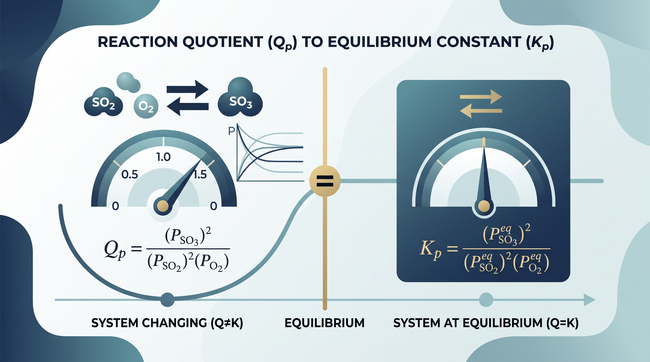
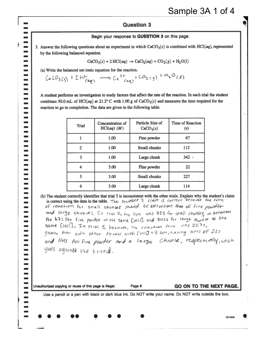
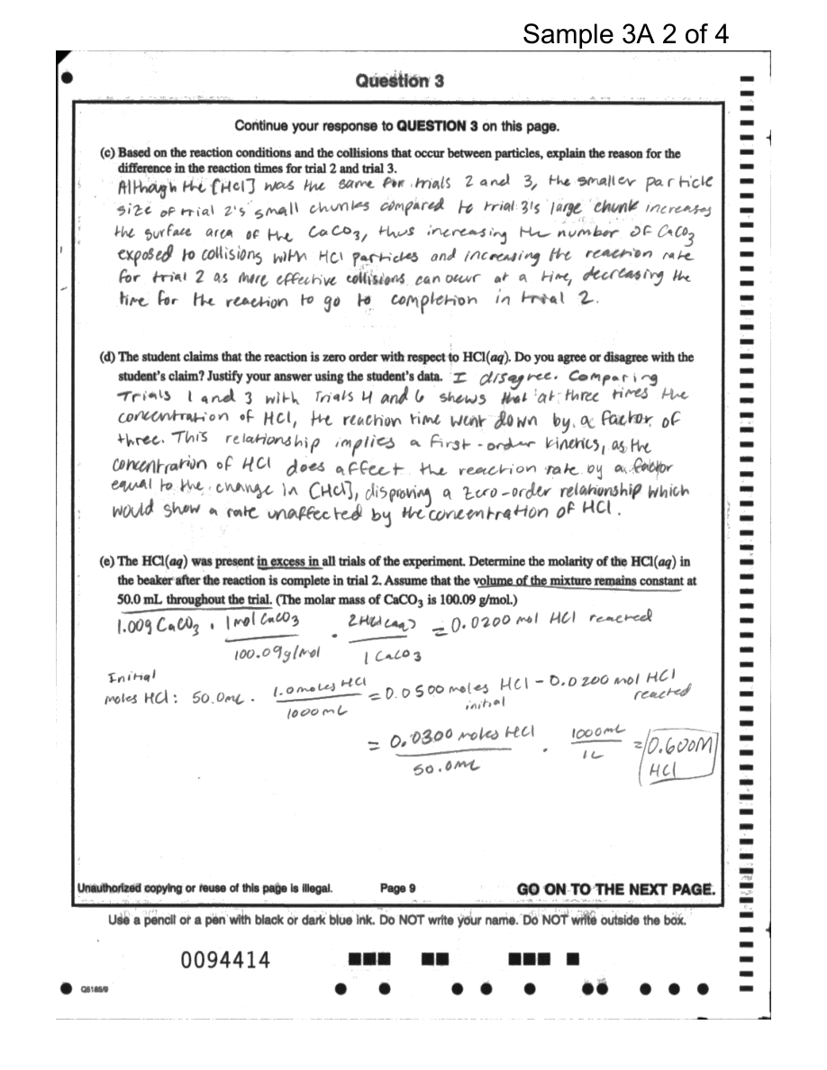
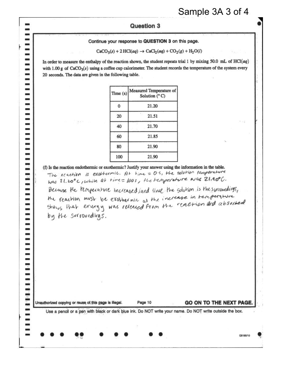
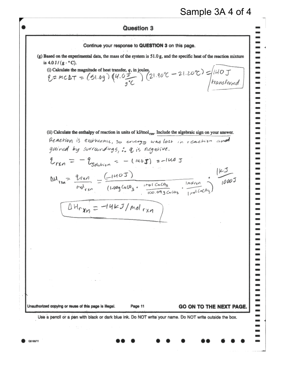
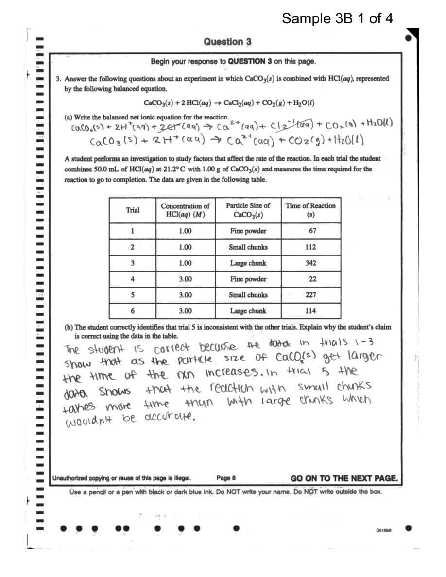
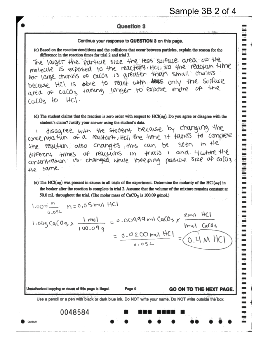
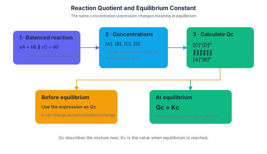
7.5 Magnitude of the Equilibrium Constant · 7.6 Properties of the Equilibrium Constant
Key concepts: Meaning of the equilibrium constant K · Relationship between the magnitude of K and the extent of a reaction · Large K (K ≫ 1) indicates products predominate at equilibrium · Small K indicates reactants predominate at equilibrium · Using equilibrium concentrations to explain concentration relationships · Equilibrium between an un-ionized weak base and its conjugate acid · Equilibrium constant Kp for reactions involving gases · Calculating an equilibrium constant from equilibrium data
At equilibrium, the value of $K$ answers a composition question: which side of the reaction contains more chemical species? It does not answer how quickly the system reaches equilibrium.
7.5 Magnitude of the Equilibrium Constant · 7.6 Properties of the Equilibrium Constant
At equilibrium, the value of $K$ answers a composition question: which side of the reaction contains more chemical species? It does not answer how quickly the system reaches equilibrium. A reaction can have a very large $K$ and still reach equilibrium slowly, or a small $K$ and reach equilibrium rapidly.
Learning Objective 7.5.A: Explain the relationship between the magnitude of the equilibrium constant and the relative concentrations of chemical species at equilibrium.
Essential Knowledge 7.5.A.1: The magnitude of the equilibrium constant indicates the relative concentrations of reactants and products present at equilibrium.
Reading the magnitude of $K$
For a general reaction,
aA+bB\rightleftharpoons cC+dD
the equilibrium constant compares product concentrations with reactant concentrations according to the reaction’s stoichiometric coefficients. The numerical value of $K$ therefore describes the equilibrium position—the mixture’s composition once the forward and reverse processes occur at equal rates.
The most useful interpretations are qualitative:
| Magnitude of $K$ | Equilibrium position | Relative composition |
|---|---|---|
| $K\gg 1$ | Far toward products | Products predominate; the reaction proceeds nearly to completion |
| $K\approx 1$ | Neither side strongly favored | Reactants and products are present in appreciable amounts |
| $K\ll 1$ | Far toward reactants | Reactants predominate; only a relatively small amount of product forms |
A large value such as $K=4.0\times10^5$ means that the product side is strongly favored. It does not mean that every reactant particle disappears: equilibrium requires some reactants and products to remain whenever the reaction is reversible. Likewise, $K=2.0\times10^{-6}$ means that reactants predominate, not that the reaction produces absolutely no product.
Misconception check: “Large $K$ means fast reaction” is incorrect. $K$ measures how far a reaction proceeds toward products; reaction rate measures how quickly it gets there. Temperature and activation energy influence rate, while the equilibrium constant at a given temperature describes equilibrium composition.
Using equilibrium concentrations as evidence
Suppose equilibrium data for
N_2O_4(g)\rightleftharpoons 2NO_2(g)
give
$$ K_c=1.25\times10^{-2}. $$
The calculation follows the equilibrium-expression method established for Topic 7.4. The important interpretation is that $K_c$ is much less than $1$, so the equilibrium mixture contains substantially more $N_2O_4$ than $NO_2$ relative to the stoichiometric relationship. The reaction lies toward the reactant side: $N_2O_4$ predominates.
That conclusion must be tied to the chemical equation, not merely to isolated concentration values. Because two moles of $NO_2$ correspond to one mole of $N_2O_4$, the comparison is weighted by the coefficients in the equilibrium expression. A statement such as “the concentration of $N_2O_4$ is larger, so $K_c$ is small” is incomplete; the stronger argument is that the calculated ratio of product terms to reactant terms is only $1.25\times10^{-2}$, demonstrating reactant-favored equilibrium.
Argumentation (6.D): A complete explanation makes a claim about which species predominate, cites the magnitude of $K$ as evidence, and connects that evidence to the balanced equation and equilibrium concentration relationship.
$K_c$ and $K_p$
For gas-phase reactions, equilibrium may be described using partial pressures rather than molar concentrations. The corresponding constant is $K_p$:
$$ K_p=\frac{(P_C)^c(P_D)^d}{(P_A)^a(P_B)^b} $$
where each $P$ is an equilibrium partial pressure. The interpretation remains the same: $K_p\gg1$ indicates products predominate, while $K_p\ll1$ indicates reactants predominate. The numerical values of $K_c$ and $K_p$ may differ because concentration and pressure use different measures, but each constant describes equilibrium composition for its chosen representation.
Weak-base equilibrium as a species relationship
A weak base illustrates how an equilibrium constant describes the relative amounts of two related species. For a weak base $B$ in water,
B(aq)+H_2O(l)\rightleftharpoons BH^+(aq)+OH^-(aq)
the un-ionized base $B$ is in equilibrium with its conjugate acid, $BH^+$. The base-ionization constant is
$$ K_b=\frac{[BH^+][OH^-]}{[B]}. $$
This is the required weak-base relationship identified in 8.3.A.4, where $K_b$ is often reported through $pK_b$:
$$ pK_b=-\log K_b. $$
Because a weak base ionizes only partially, $[B]$ remains much larger than the concentrations of $BH^+$ and $OH^-$ at equilibrium. Thus, a small $K_b$ indicates that the equilibrium lies mostly toward the un-ionized base. The phrase “weak” refers to limited ionization at equilibrium—not to a slow reaction.
Retrieval check
For the reaction
X_2(g)\rightleftharpoons 2X(g),
a calculated value of $K_p=3.0\times10^{-7}$ is obtained from equilibrium partial pressures. Which species predominates, and what evidence supports the conclusion? The answer should identify $X_2$ as predominant and explain that $K_p\ll1$, so the equilibrium position lies strongly toward reactants.
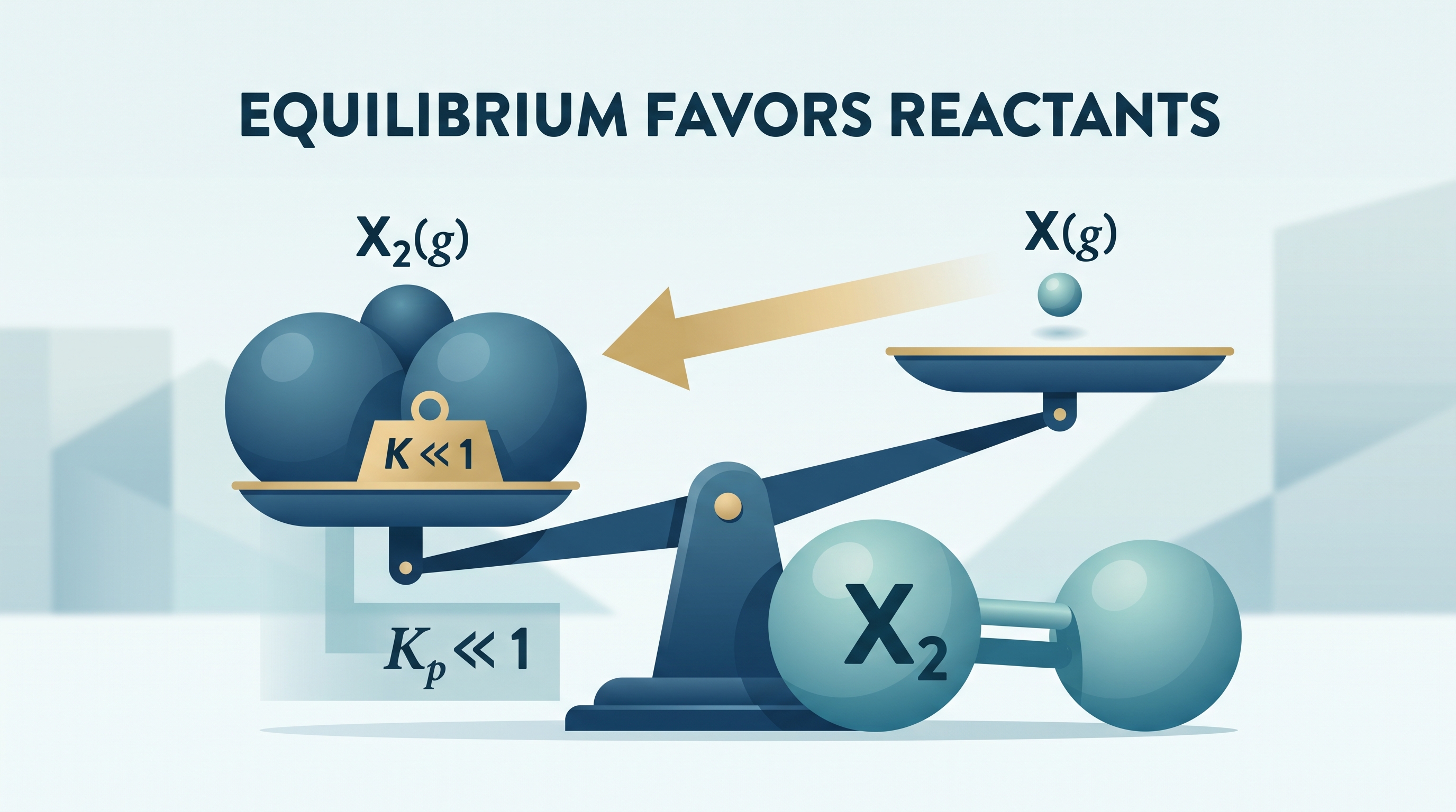
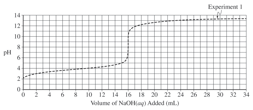
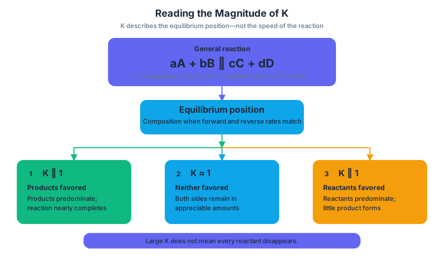
7.7 Calculating Equilibrium Concentrations · 7.8 Representations of Equilibrium
Key concepts: Writing equilibrium constant expressions from balanced chemical equations · Calculating equilibrium concentrations using stoichiometry and equilibrium relationships · Distinguishing equilibrium concentrations from initial concentrations · Calculating and interpreting the reaction quotient Q · Comparing Q with K to predict the direction of equilibrium shift · Applying Le Châtelier’s principle to stress an equilibrium system · Representing equilibrium at the particulate level · Using stoichiometric coefficients to determine ion ratios in solution · Calculating solubility equilibria with Ksp · Recognizing common student errors in equilibrium calculations and diagrams
At equilibrium, a reaction mixture is not “finished”: particles continue colliding and reacting in both directions, while the macroscopic concentrations remain constant. The central calculation is therefore to connect a balanced equation, concentration changes, and the equilibrium constant.
7.7 Calculating Equilibrium Concentrations · 7.8 Representations of Equilibrium
At equilibrium, a reaction mixture is not “finished”: particles continue colliding and reacting in both directions, while the macroscopic concentrations remain constant. The central calculation is therefore to connect a balanced equation, concentration changes, and the equilibrium constant.
Learning Objective 7.7: The student is able to calculate equilibrium concentrations by applying stoichiometry and the equilibrium constant expression.
Essential Knowledge 7.7.A: The equilibrium constant expression relates equilibrium concentrations of reactants and products.
Learning Objective 7.8: The student is able to use representations to describe the relationships between the concentrations of reactants and products in an equilibrium system.
Essential Knowledge 7.8.A: Representations of equilibrium must agree with the balanced equation and its stoichiometric relationships.
From a balanced equation to an equilibrium expression
For the general reaction
aA+bB\rightleftharpoons cC+dD
the concentration-based equilibrium constant is
$$ K_c=\frac{[C]^c[D]^d}{[A]^a[B]^b}. $$
The exponents are the stoichiometric coefficients from the balanced equation. Pure solids and pure liquids are omitted because their effective concentrations remain constant.
For example,
Sr(OH)_2(s)\rightleftharpoons Sr^{2+}(aq)+2OH^-(aq)
has
$$ K_{sp}=[Sr^{2+}][OH^-]^2. $$
The solid $Sr(OH)_2$ does not appear. If a saturated solution contains $[Sr^{2+}]=0.043\ \mathrm{M}$, the balanced equation requires
$$ [OH^-]=2(0.043\ \mathrm{M})=0.086\ \mathrm{M}. $$
Thus,
$$ K_{sp}=(0.043)(0.086)^2=3.18\times10^{-4}. $$
Misconception check — “The ions dissolve in a $1:1$ ratio.” They do not. Each formula unit produces one $Sr^{2+}$ ion and two $OH^-$ ions. A particulate model must therefore show twice as many hydroxide ions as strontium ions.
Calculating equilibrium concentrations with an ICE relationship
An ICE relationship records initial concentration, change, and equilibrium concentration. The change row comes directly from stoichiometry; the equilibrium row combines the initial amount with the unknown change.
Consider
N_2O_4(g)\rightleftharpoons 2NO_2(g)
with initial concentrations $[N_2O_4]_0=1.00\ \mathrm{M}$ and $[NO_2]_0=0$, and $K_c=0.36$.
| Species | Initial | Change | Equilibrium |
|---|---|---|---|
| $N_2O_4$ | $1.00$ | $-x$ | $1.00-x$ |
| $NO_2$ | $0$ | $+2x$ | $2x$ |
Substitute the equilibrium concentrations into the expression:
$$ 0.36=\frac{[NO_2]^2}{[N_2O_4]} =\frac{(2x)^2}{1.00-x}. $$
Solving gives $x=0.258$ (the negative mathematical root is chemically impossible). Therefore,
$$ [N_2O_4]_{\mathrm{eq}}=1.00-0.258=0.742\ \mathrm{M} $$
and
$$ [NO_2]_{\mathrm{eq}}=2(0.258)=0.517\ \mathrm{M}. $$
Equilibrium check:
$$ K_c=\frac{(0.517)^2}{0.742}=0.360\approx0.36. $$
The result is self-consistent. Notice that $NO_2$ changes by $2x$, not $x$; losing that coefficient produces an incorrect equilibrium composition even if the algebra is flawless.
The reaction quotient predicts the net direction
The reaction quotient, $Q$, has the same concentration form as $K$, but it uses concentrations that are not necessarily at equilibrium:
$$ Q_c=\frac{[C]^c[D]^d}{[A]^a[B]^b}. $$
Compare $Q$ with the already-known value of $K$:
- If $Q<K$, the mixture contains too much reactant relative to equilibrium, so the net reaction proceeds toward products.
- If $Q>K$, the mixture contains too much product, so the net reaction proceeds toward reactants.
- If $Q=K$, the system is at equilibrium.
For the $N_2O_4/NO_2$ system, suppose the current concentrations are $[N_2O_4]=0.80\ \mathrm{M}$ and $[NO_2]=0.20\ \mathrm{M}$:
$$ Q_c=\frac{(0.20)^2}{0.80}=0.050. $$
Because $0.050<0.36$, the net change is toward products: more $N_2O_4$ dissociates to form $NO_2$ until $Q$ rises to $K$.
Representations must preserve stoichiometry
A correct equilibrium representation can be symbolic, graphical, particulate, or numerical, but all representations must tell the same chemical story. For $N_2O_4\rightleftharpoons2NO_2$, a particle diagram must represent each $N_2O_4$ molecule as one unit and each dissociation event as two $NO_2$ molecules; a $1:1$ product ratio contradicts the equation.
A specific stress can temporarily make $Q\ne K$. For example, adding $N_2O_4$ increases the denominator of
$$ Q_c=\frac{[NO_2]^2}{[N_2O_4]}, $$
so $Q$ becomes less than $K$. The system responds by shifting toward $NO_2$, restoring $Q=K$; the value of $K$ itself changes only if temperature changes.
Retrieval check: For
A(s)\rightleftharpoons2B(aq),
write the equilibrium expression, state the concentration change if $[A]$ dissolves by $x$, and predict the direction when $Q>K$.
Answer: $K=[B]^2$; $[B]$ changes by $+2x$; the system shifts toward reactants.
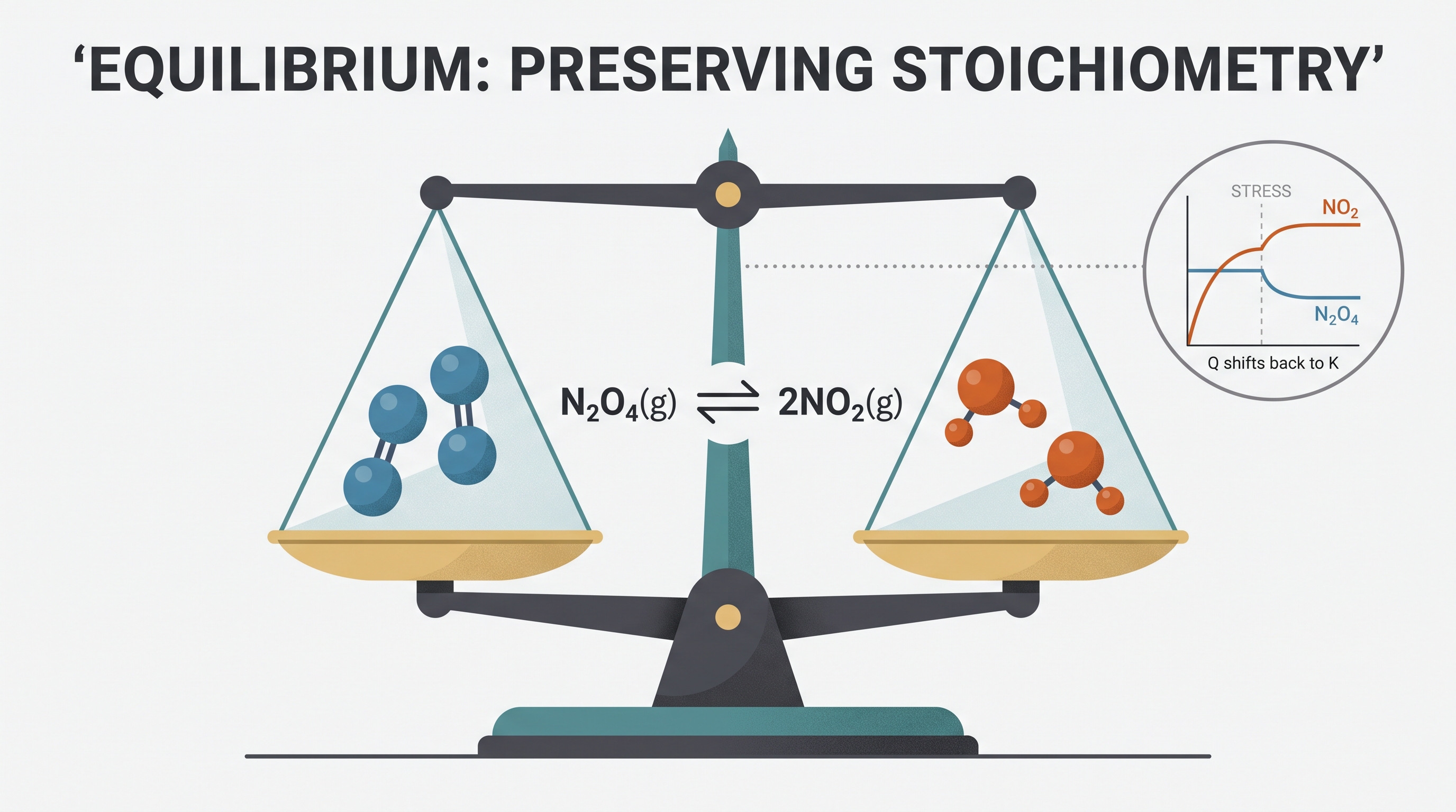
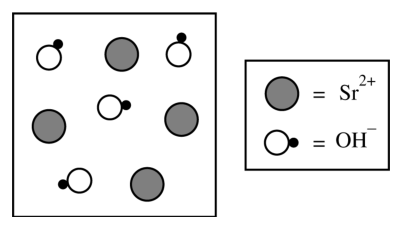
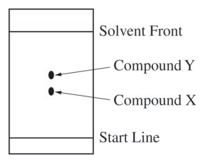
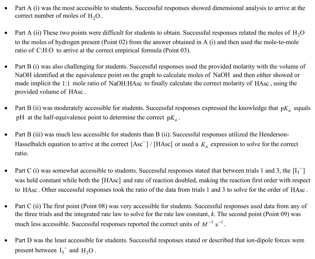
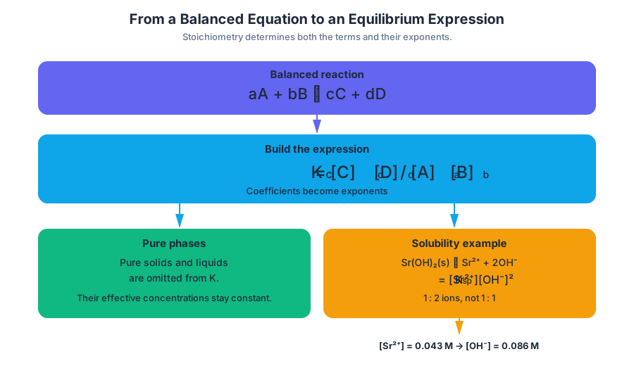
7.9 Introduction to Le Châtelier’s Principle · 7.10 Reaction Quotient and Le Châtelier’s Principle
Key concepts: Le Châtelier’s principle · Dynamic chemical equilibrium · Reaction quotient (Q) and equilibrium constant (K) · Effects of concentration disturbances on equilibrium · Effects of pressure and volume changes on gaseous equilibria · Redistribution of species to restore equilibrium · Equilibrium shifts in response to removing a species · Solubility equilibria · Interpreting macroscopic and particle-level changes · Using equilibrium reasoning to explain changes in amount and concentration
A chemical equilibrium is not frozen: particles continue reacting in both directions, but the forward and reverse reaction rates are equal. The system appears unchanged because its composition is dynamically maintained.
7.9 Introduction to Le Châtelier’s Principle · 7.10 Reaction Quotient and Le Châtelier’s Principle
A chemical equilibrium is not frozen: particles continue reacting in both directions, but the forward and reverse reaction rates are equal. The system appears unchanged because its composition is dynamically maintained.
Le Châtelier’s principle: When an equilibrium system is disturbed, the system responds by shifting in the direction that reduces the effect of the disturbance.
The most precise way to predict that shift is to compare the reaction quotient, $Q$, with the equilibrium constant, $K$.
For a general reaction,
aA+bB\rightleftharpoons cC+dD
the reaction quotient has the same form as the equilibrium-constant expression:
$$ Q=\frac{[C]^c[D]^d}{[A]^a[B]^b} $$
At equilibrium,
$$ Q=K $$
A disturbance changes one or more concentrations or partial pressures. Immediately afterward, $Q$ usually no longer equals $K$, and the reaction proceeds in whichever direction restores equality.
The $Q$–$K$ decision rule
The three cases below replace vague “shift left” or “shift right” intuition with a testable prediction.
| Comparison after disturbance | System response | Chemical interpretation |
|---|---|---|
| $Q<K$ | Proceeds toward products | $Q$ must increase |
| $Q>K$ | Proceeds toward reactants | $Q$ must decrease |
| $Q=K$ | No net shift | The system is already at equilibrium |
The concentrations may change while the system re-equilibrates, but at the new equilibrium the final quotient again satisfies $Q=K$. For a temperature change, the value of $K$ itself changes; for a concentration or pressure disturbance, $K$ remains constant at the same temperature.
Worked example: adding a product
Consider
H_2(g)+I_2(g)\rightleftharpoons 2HI(g)
with
$$ Q=\frac{[HI]^2}{[H_2][I_2]} $$
If additional $HI$ is injected, the numerator increases immediately while the denominator is initially unchanged. Therefore $Q$ becomes larger than $K$:
$$ Q>K $$
The system consumes some $HI$ and produces $H_2$ and $I_2$, shifting toward reactants until $Q$ returns to $K$. Saying “the equilibrium shifts left” is incomplete unless it identifies the particle-level change: $HI$ decreases while $H_2$ and $I_2$ increase during the response.
Misconception check — “The reaction stops at equilibrium.” Equilibrium means equal rates, not equal concentrations and not zero reaction. Both directions continue, while the concentrations remain constant overall.
Concentration disturbances and a saturated magnesium hydroxide system
A saturated solution containing undissolved magnesium hydroxide can be represented by
Mg(OH)_2(s)\rightleftharpoons Mg^{2+}(aq)+2OH^-(aq)
The solid does not appear in the reaction quotient because the activity of a pure solid is treated as constant. Thus,
$$ Q=\left[Mg^{2+}\right]\left[OH^-\right]^2 $$
Suppose acid is added. The hydrogen ions react with hydroxide ions:
$$ H^+(aq)+OH^-(aq)\rightarrow H_2O(l) $$
Removing $OH^-$ decreases the numerator of $Q$, so immediately,
$$ Q<K $$
The system responds by dissolving more $Mg(OH)_2(s)$, producing additional $Mg^{2+}$ and $OH^-$. Therefore, the amount of undissolved solid decreases. The observable pH also changes because hydroxide has been consumed.
This reasoning is stronger than saying simply “the equilibrium shifts right.” It connects the observable disturbance—adding acid—to the particle-level event—hydroxide removal—and then to the macroscopic result—more solid dissolves.
Pressure and volume changes in gaseous equilibria
Changing the container volume changes the partial pressures of all gases. A decrease in volume raises every partial pressure; an increase in volume lowers every partial pressure. The equilibrium response depends on the total gaseous coefficients on each side.
For
there are two moles of gaseous reactants and two moles of gaseous products:
$$ \Delta n_{\text{gas}}=2-2=0 $$
If the volume changes, every gas concentration changes by the same factor. In the quotient,
$$ Q=\frac{[HI]^2}{[H_2][I_2]} $$
the common factor cancels, so $Q$ remains equal to $K$. There is no equilibrium shift, and the amount of $HI$ remains unchanged.
Reading an observable change
If an experiment reports that the moles of $HI(g)$ increase, that is evidence that the system moved toward products, meaning more $H_2$ and $I_2$ were converted into $HI$. Do not call $H_2$ and $I_2$ products: they are reactants in the written equation, while $HI$ is the product.
Misconception check — “Higher pressure always favors products.” Pressure changes favor the side with fewer gaseous moles only when the two sides have different gas totals. When $\Delta n_{\text{gas}}=0$, pressure or volume changes do not alter the equilibrium position.
AP Chemistry reasoning: 7.10.A and 5.F
Learning Objective 7.10.A requires explaining the relationship among $Q$, $K$, and the direction in which a reversible reaction proceeds to reach equilibrium.
Essential Knowledge 7.10.A.1: A disturbance causes $Q$ to differ from $K$, taking the system out of equilibrium; the system responds by bringing $Q$ back into agreement with $K$.
Essential Knowledge 7.10.A.2: Concentration changes generally change $Q$ only, whereas temperature changes $K$; in either case, species redistribute until $Q$ and $K$ are equal again.
Suggested Skill 5.F: Mathematical Routines is assessed when you calculate, estimate, or predict an unknown quantity by selecting a logical computational pathway and attending to precision. Here, the pathway is: write $Q$, identify what changed, compare $Q$ with $K$, and predict the direction of redistribution.
Retrieval check: For the magnesium hydroxide equilibrium, acid removes $OH^-$. Does $Q$ become greater than, less than, or equal to $K$? What happens to the amount of solid? For the hydrogen–iodine equilibrium, why does increasing volume leave the amount of $HI$ unchanged?
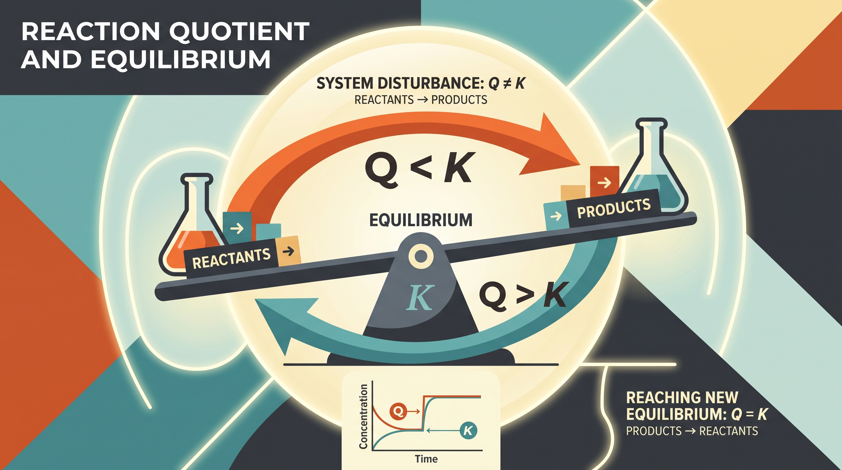
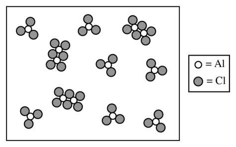
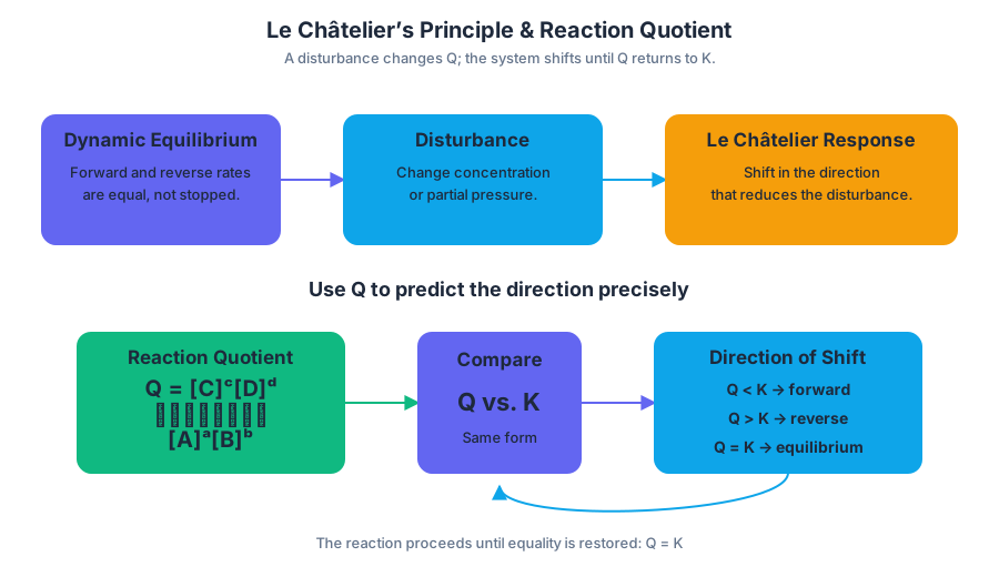
7.11 Introduction to Solubility Equilibria · 7.12 Common-Ion Effect
Key concepts: Solubility equilibria · Solubility product constant (Ksp) · Molar solubility · Relationship between Ksp and molar solubility · Common-ion effect · Le Châtelier’s principle · Dissolution equilibria · Qualitative solubility rules · Calculating solubility from Ksp · Effect of modifying solution composition on experimental results
A sparingly soluble salt does not simply “stop dissolving”; it reaches a dynamic balance in which solid dissolves and dissolved ions recombine at equal rates.
7.11 Introduction to Solubility Equilibria · 7.12 Common-Ion Effect
A sparingly soluble salt does not simply “stop dissolving”; it reaches a dynamic balance in which solid dissolves and dissolved ions recombine at equal rates.
The dissolution equilibrium
For a salt such as silver chloride, the equilibrium is
$$ \mathrm{AgCl(s)\rightleftharpoons Ag^+(aq)+Cl^-(aq)} $$
At equilibrium, some solid remains while ions are present in solution. The solubility product constant, $K_{sp}$, is the equilibrium constant for this dissolution process:
$$ K_{sp}=[\mathrm{Ag^+}][\mathrm{Cl^-}] $$
The solid $\mathrm{AgCl}$ does not appear in the expression because the concentration of a pure solid is effectively constant.
The stoichiometric coefficients in the dissolution equation become exponents in the $K_{sp}$ expression. For calcium fluoride,
$$ \mathrm{CaF_2(s)\rightleftharpoons Ca^{2+}(aq)+2F^-(aq)} $$
so
$$ K_{sp}=[\mathrm{Ca^{2+}}][\mathrm{F^-}]^2 $$
The exponent on fluoride is not optional: two fluoride ions are produced for every calcium ion.
Molar solubility and $K_{sp}$
Molar solubility is the number of moles of salt that dissolve per liter of solution. If the molar solubility of $\mathrm{CaF_2}$ is $s$, then dissolving $s$ moles per liter produces $s$ moles per liter of $\mathrm{Ca^{2+}}$ and $2s$ moles per liter of $\mathrm{F^-}$:
$$ [\mathrm{Ca^{2+}}]=s \qquad [\mathrm{F^-}]=2s $$
Substitution gives
$$ K_{sp}=s(2s)^2=4s^3 $$
For $K_{sp}=3.2\times10^{-11}$,
$$ s=\sqrt[3]{\frac{3.2\times10^{-11}}{4}} =2.0\times10^{-4}\ \mathrm{M} $$
Thus the molar solubility is $2.0\times10^{-4}\ \mathrm{M}$, while the equilibrium fluoride concentration is $4.0\times10^{-4}\ \mathrm{M}$.
Misconception check — $K_{sp}$ is not the same as solubility. A smaller $K_{sp}$ usually indicates a less soluble salt within a comparable stoichiometric pattern, but $K_{sp}$ and molar solubility have different meanings and units. Also, comparing numerical $K_{sp}$ values across salts with different formulas can be misleading because their ion concentrations enter the expressions differently.
The common-ion effect
The common-ion effect occurs when a solution already contains an ion produced by a dissolving salt. Adding that ion decreases the salt’s solubility. This is required by the equilibrium expression, not an exception to it.
For $\mathrm{AgCl}$,
adding $\mathrm{NaCl}$ increases $[\mathrm{Cl^-}]$. The product $[\mathrm{Ag^+}][\mathrm{Cl^-}]$ would then exceed $K_{sp}$, so some $\mathrm{Ag^+}$ and $\mathrm{Cl^-}$ combine to form more $\mathrm{AgCl(s)}$. The equilibrium shifts left, and less solid dissolves.
This is the solubility-equilibrium application of Le Châtelier’s principle: adding a product favors the direction that consumes that product. The solid forms until the ion product again equals $K_{sp}$.
Quantitative common-ion calculation
Suppose $K_{sp}$ for $\mathrm{AgCl}$ is $1.8\times10^{-10}$ and the solution already contains $0.010\ \mathrm{M}$ $\mathrm{Cl^-}$ from $\mathrm{NaCl}$. Let $s$ be the additional concentration of $\mathrm{AgCl}$ that dissolves:
$$ [\mathrm{Ag^+}]=s \qquad [\mathrm{Cl^-}]\approx0.010 $$
The approximation is valid because the added $0.010\ \mathrm{M}$ chloride is much larger than the tiny amount supplied by dissolution.
$$ K_{sp}=s(0.010) $$
$$ s=\frac{1.8\times10^{-10}}{0.010} =1.8\times10^{-8}\ \mathrm{M} $$
In pure water, the molar solubility would be approximately $\sqrt{K_{sp}}=1.3\times10^{-5}\ \mathrm{M}$. The common ion reduces the solubility by roughly three orders of magnitude.
Solubility rules versus solubility equilibria
Qualitative solubility rules classify substances as generally soluble or insoluble; they do not replace an equilibrium calculation. A “soluble” salt can still have a finite saturation concentration, and a “slightly soluble” salt still dissolves to some extent. Use $K_{sp}$ when the problem supplies equilibrium data or asks for a numerical solubility.
The RbCl example illustrates this distinction. RbCl is classified as soluble, so its molar solubility is not normally treated as a small $K_{sp}$-controlled quantity in water at $20^\circ\mathrm{C}$. KCl contains the common ion $\mathrm{Cl^-}$, so a formal common-ion argument is chemically relevant; however, ordinary AP reasoning should not invent a numerical $K_{sp}$ for RbCl when none is provided. The defensible conclusion is that the experiment must distinguish a measurable saturation change from the qualitative prediction for a sparingly soluble salt.
Experimental consequences and AP skill
Changing the solvent, adding a common-ion source, altering concentrations, or failing to control temperature can change the measured solubility. For example, measuring the solubility of $\mathrm{AgCl}$ in pure water and then repeating the measurement in $\mathrm{NaCl}$ solution should produce a smaller dissolved amount and potentially more solid precipitate.
This topic develops Learning Objective 7.12.A: “Identify the solubility of a salt, and/or the value of $K_{sp}$ for the salt, based on the concentration of a common ion already present in solution.” It also applies Essential Knowledge 7.12.A.1, which states that a salt’s solubility is reduced when the solution already contains one of its ions and that the effect can be explained qualitatively with Le Châtelier’s principle or calculated from $K_{sp}$.
The relevant science practice is 2.F — Explain how modifications to an experimental procedure will alter results. A strong response names the changed ion concentration, connects it to the $K_{sp}$ expression, predicts the equilibrium shift, and states the observable consequence.
Retrieval check: For $\mathrm{PbI_2(s)\rightleftharpoons Pb^{2+}(aq)+2I^-(aq)}$, write $K_{sp}$ and predict what happens when $\mathrm{KI(aq)}$ is added. The expression is $K_{sp}=[\mathrm{Pb^{2+}}][\mathrm{I^-}]^2$; adding $\mathrm{I^-}$ shifts the equilibrium toward $\mathrm{PbI_2(s)}$, decreasing its molar solubility.
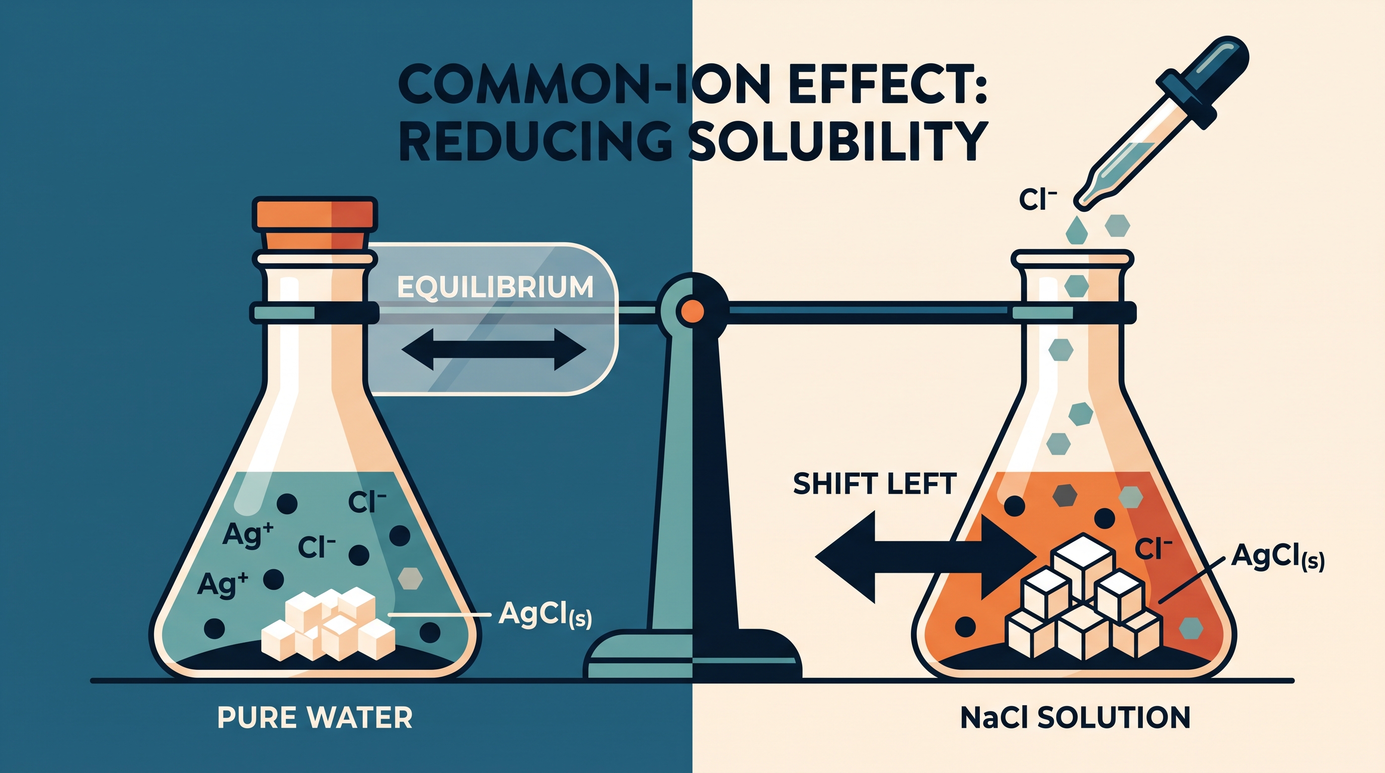
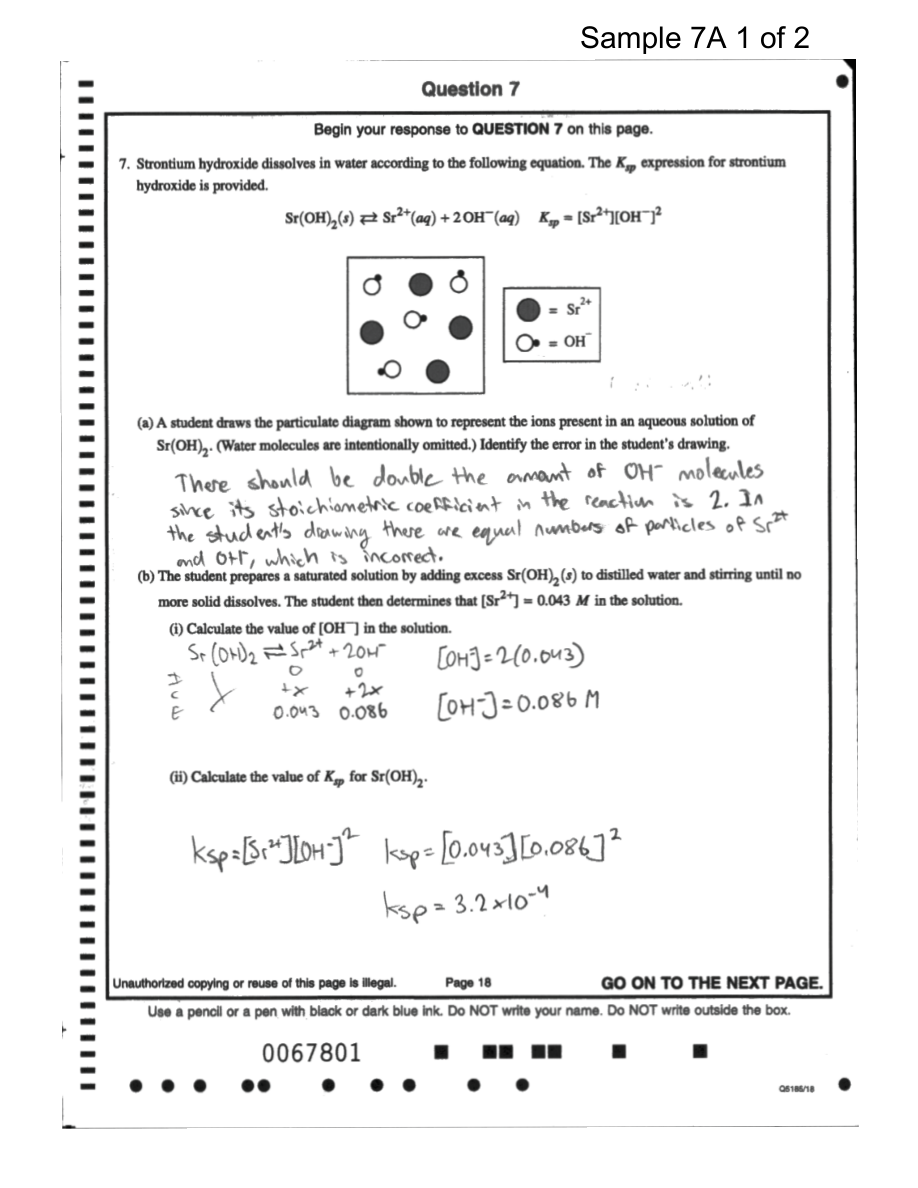
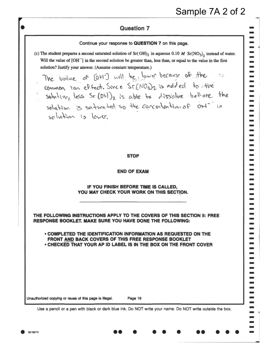
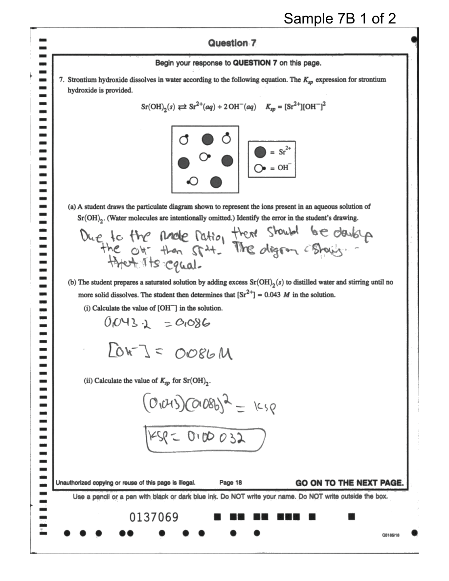
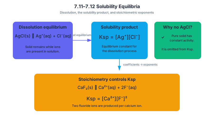
8.1 Introduction to Acids and Bases · 8.2 pH and pOH of Strong Acids and Bases
Key concepts: Definitions and introductory concepts of acids and bases · Strong acids and strong bases · Ionization/dissociation of strong bases in aqueous solution · pH and pOH · The water ionization constant, Kw · Neutral aqueous solutions · Concentrations of all species in a neutral solution of water · Group 1 hydroxides as strong bases · Group 2 hydroxides as strong bases · Use of indicators to distinguish acidic and basic solutions
Acids and bases are distinguished by which ions they create or consume in water: an acid increases hydronium ions, while a base increases hydroxide ions or accepts protons.
8.1 Introduction to Acids and Bases · 8.2 pH and pOH of Strong Acids and Bases
Acids and bases are distinguished by which ions they create or consume in water: an acid increases hydronium ions, while a base increases hydroxide ions or accepts protons. Those tiny ion-concentration changes control everything from the sharpness of citrus juice to the cleaning power of drain products.
Two ways to define acids and bases
The Arrhenius definition describes aqueous solutions directly:
- An Arrhenius acid increases the concentration of hydronium, $H_3O^+$, in water.
- An Arrhenius base increases the concentration of hydroxide, $OH^-$, in water.
The Brønsted–Lowry definition focuses on proton transfer:
- A Brønsted–Lowry acid donates a proton, $H^+$.
- A Brønsted–Lowry base accepts a proton, $H^+$.
In aqueous solution, a donated proton does not normally float alone. It attaches to a water molecule:
$$ H^+ + H_2O \rightarrow H_3O^+ $$
Thus, “hydrogen ion” and “hydronium ion” are used interchangeably for AP Chemistry calculations, although $H_3O^+$ is the more chemically precise notation.
A solution is acidic when $[H_3O^+] > [OH^-]$, basic when $[OH^-] > [H_3O^+]$, and neutral when the two concentrations are equal. The solvent water itself remains overwhelmingly more abundant than either ion.
Water autoionization and neutrality
Water molecules continuously exchange protons in a reversible process called autoionization:
2H_2O \rightleftharpoons H_3O^+ + OH^-
The equilibrium relationship is the water ionization constant, $K_w$:
$$ K_w = [H_3O^+][OH^-] $$
At $25^\circ\text{C}$,
$$ K_w = 1.0 \times 10^{-14} $$
For pure neutral water at this temperature,
$$ [H_3O^+] = [OH^-] = 1.0 \times 10^{-7}\ \text{M} $$
The concentration of un-ionized water is approximately
$$ [H_2O] \approx 55.5\ \text{M} $$
Because $55.5\ \text{M}$ is vastly larger than $1.0 \times 10^{-7}\ \text{M}$, the solvent-water concentration is treated as effectively constant in aqueous equilibrium calculations. Neutral does not mean that no ions are present; it means equal concentrations of hydronium and hydroxide.
8.1.A.1: Hydronium and hydroxide concentrations are expressed using the logarithmic scales pH and pOH.
8.1.A.2: At $25^\circ\text{C}$, $K_w = [H_3O^+][OH^-] = 1.0 \times 10^{-14}$.
Taking negative logarithms gives the useful relationship
$$ \text{pH} = -\log[H_3O^+] $$
$$ \text{pOH} = -\log[OH^-] $$
At $25^\circ\text{C}$,
$$ \text{pH} + \text{pOH} = \text{p}K_w = 14.00 $$
The value $14.00$ is temperature-specific: do not assume that neutral water has pH $7.00$ at every temperature.
Strong acids: complete ionization
A strong acid ionizes essentially completely in water. Common examples include $HCl$, $HBr$, $HI$, $HClO_4$, $H_2SO_4$, and $HNO_3$. For a monoprotic strong acid such as hydrochloric acid,
$$ HCl + H_2O \rightarrow H_3O^+ + Cl^- $$
A $0.010\ \text{M}$ solution of $HCl$ therefore has
$$ [H_3O^+] \approx 0.010\ \text{M} $$
and
$$ \text{pH} = -\log(1.0 \times 10^{-2}) = 2.00 $$
The concentration of the conjugate base, $[Cl^-]$, is also approximately $0.010\ \text{M}$.
8.2.A.1: Molecules of a strong acid completely ionize in aqueous solution, so the hydronium concentration is related directly to the initial strong-acid concentration.
Strong bases: complete dissociation
Strong bases such as Group $1$ and Group $2$ hydroxides dissociate essentially completely. The subscript on the hydroxide compound determines how many hydroxide ions each formula unit produces.
For a Group $1$ hydroxide:
$$ NaOH \rightarrow Na^+ + OH^- $$
Thus, a $0.020\ \text{M}$ $NaOH$ solution has
$$ [OH^-] = 0.020\ \text{M} $$
$$ \text{pOH} = -\log(2.0 \times 10^{-2}) = 1.70 $$
$$ \text{pH} = 14.00 - 1.70 = 12.30 $$
For a Group $2$ hydroxide:
$$ Ca(OH)_2 \rightarrow Ca^{2+} + 2OH^- $$
A $0.020\ \text{M}$ $Ca(OH)_2$ solution produces twice as many hydroxide ions:
$$ [OH^-] = 2(0.020) = 0.040\ \text{M} $$
Then
$$ \text{pOH} = -\log(0.040) = 1.40 $$
and
$$ \text{pH} = 14.00 - 1.40 = 12.60 $$
8.2.A.2: Strong bases completely dissociate to produce hydroxide ions; for a Group $1$ hydroxide, $[OH^-]$ equals the initial compound concentration, while for a Group $2$ hydroxide, $[OH^-]$ is twice that concentration.
Indicator evidence and a logarithmic misconception
Universal indicator provides a visible particle-level clue: acidic solutions tend toward red or orange, basic solutions toward blue or purple, and a buffered solution shows a color corresponding to its pH while resisting rapid color change when small amounts of acid or base are added. The color is evidence of relative hydronium and hydroxide concentrations, not a direct measurement of molarity.
Misconception check: If $\text{pH}=3.00$, the solution does not contain $3.00\ \text{M}$ hydronium. Instead,
$$ [H_3O^+] = 10^{-3.00}\ \text{M} = 1.0 \times 10^{-3}\ \text{M} $$
pH is a logarithmic measure, so a one-unit decrease in pH means a tenfold increase in hydronium concentration.
Retrieval check
A solution contains $0.0050\ \text{M}$ $KOH$. Identify $[OH^-]$, pOH, and pH. Because $KOH$ is a Group $1$ strong base, $[OH^-]=0.0050\ \text{M}$; therefore $\text{pOH}=2.30$ and, at $25^\circ\text{C}$, $\text{pH}=11.70$.
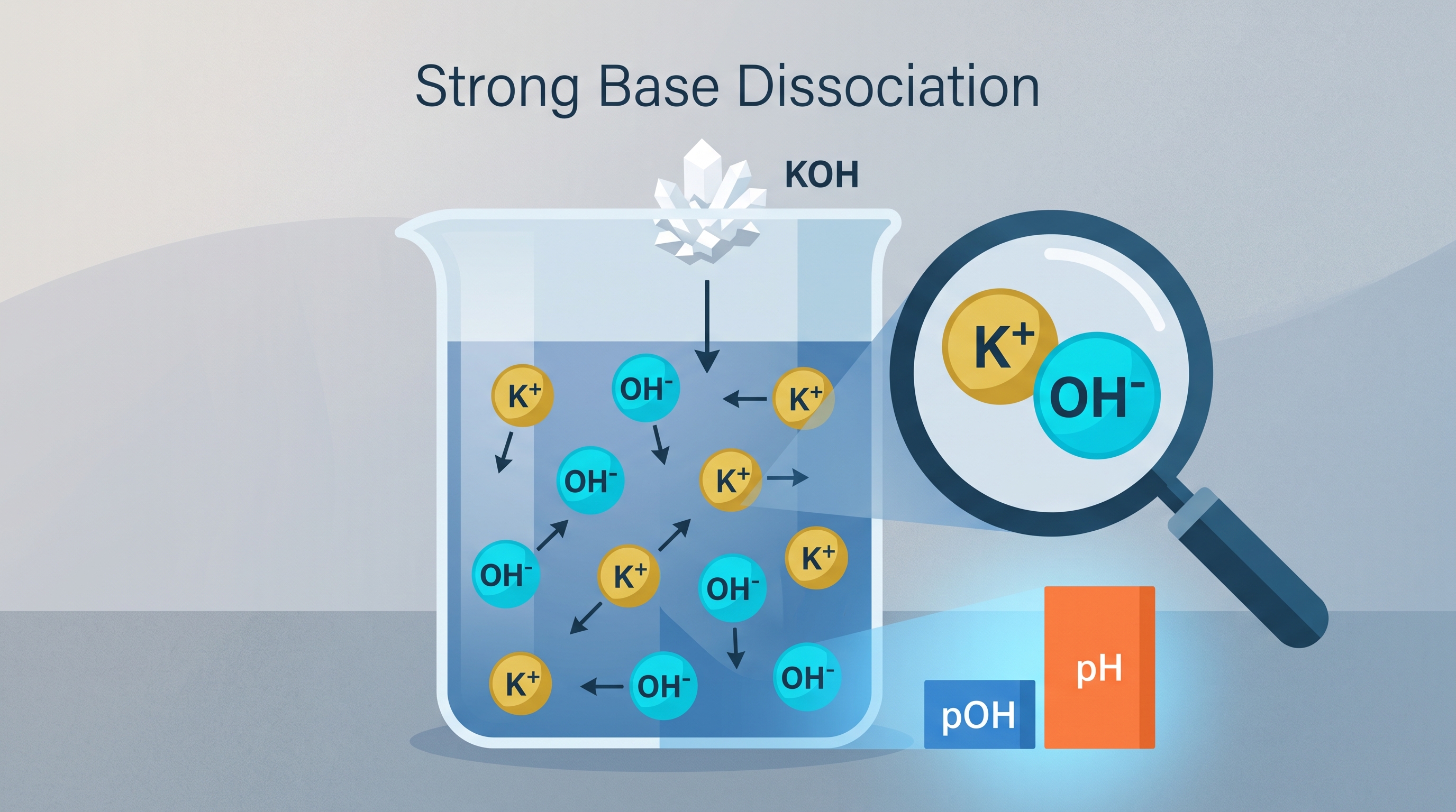
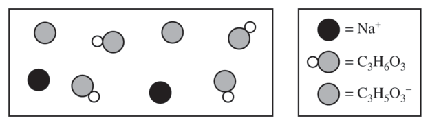
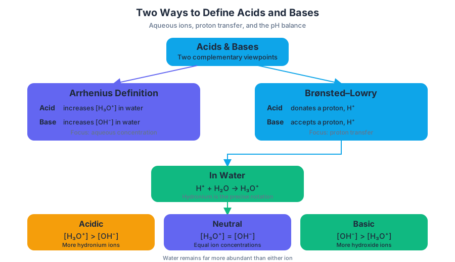
8.3 Weak Acid and Base Equilibria · 8.4 Acid-Base Reactions and Buffers
Key concepts: Weak acid equilibria and acid ionization constant (Ka) · Weak base equilibria and base ionization constant (Kb) · pKa and pKb as logarithmic measures of Ka and Kb · Percent ionization of weak acids and bases · Equilibrium concentrations of major species in acid-base solutions · Quantitative acid-base reactions and limiting/excess reagents · Buffer solutions composed of a weak acid/base and its conjugate partner · pH determination after mixing weak acids or bases with strong reagents · Equimolar weak base–strong acid mixtures and the acidic conjugate-acid equilibrium · Buffer capacity for added acid versus added base
A solution’s pH depends not only on which acid is present, but also on how extensively that acid transfers protons to water. Equal-concentration solutions of hydrochloric acid, carbonic acid, $H_2CO_3$, and acetic acid, $HC_2H_3O_2$, do not produce equal hydronium concentrations because strong acids ionize…
8.3 Weak Acid and Base Equilibria · 8.4 Acid-Base Reactions and Buffers
A solution’s pH depends not only on which acid is present, but also on how extensively that acid transfers protons to water. Equal-concentration solutions of hydrochloric acid, carbonic acid, $H_2CO_3$, and acetic acid, $HC_2H_3O_2$, do not produce equal hydronium concentrations because strong acids ionize essentially completely while weak acids ionize only partially.
Weak-acid equilibrium: partial ionization, not incomplete reaction
A weak acid is an acid that transfers only a fraction of its available protons to water. Most particles remain as un-ionized $HA$, while smaller amounts become hydronium, $H_3O^+$, and the conjugate base, $A^-$.
The equilibrium is represented by
HA(aq) + H_2O(l) \rightleftharpoons H_3O^+(aq) + A^-(aq)
The acid ionization constant, $K_a$, measures the extent of this ionization:
$$ K_a=\frac{[H_3O^+][A^-]}{[HA]} $$
Liquid water is omitted because its concentration is effectively constant. A larger $K_a$ means a greater equilibrium tendency to form $H_3O^+$ and $A^-$, so the acid is stronger. The logarithmic measure is
$$ pK_a=-\log K_a $$
Because of the negative sign, smaller $pK_a$ means stronger acid. The common mistake is to use the initial acid concentration as the final hydronium concentration. For a weak acid, most of the initial acid remains $HA$, so $[H_3O^+]$ is significantly smaller than the initial $[HA]$.
Worked example: percent ionization of a weak acid
Suppose $0.100\ \mathrm{M}$ acetic acid has $K_a=1.8\times10^{-5}$. Let $x$ represent the amount of acid that ionizes.
At equilibrium:
$$ [H_3O^+]=x,\qquad [C_2H_3O_2^-]=x,\qquad [HC_2H_3O_2]=0.100-x $$
Substitution into the $K_a$ expression gives
$$ 1.8\times10^{-5}=\frac{x^2}{0.100-x} $$
Because $K_a$ is small, $x$ is much smaller than $0.100$, so $0.100-x\approx0.100$:
$$ x\approx\sqrt{(1.8\times10^{-5})(0.100)} =1.34\times10^{-3}\ \mathrm{M} $$
Thus,
$$ %\ \mathrm{ionization} =\frac{[H_3O^+]{\mathrm{eq}}}{[HA]{\mathrm{initial}}}\times100 =\frac{1.34\times10^{-3}}{0.100}\times100 =1.34% $$
Only about $1.34%$ of the acid ionizes, even though the solution is acidic. Misconception check: “Weak” does not mean “dilute,” and it does not mean “harmless.” It describes the fraction ionized at equilibrium.
Weak-base equilibrium and conjugate-acid behavior
A weak base accepts protons from water only partially. Its equilibrium is
B(aq)+H_2O(l)\rightleftharpoons HB^+(aq)+OH^-(aq)
The base ionization constant, $K_b$, is
$$ K_b=\frac{[HB^+][OH^-]}{[B]} $$
For a weak base, the equilibrium concentration of $OH^-$ does not equal the initial concentration of $B$. Most base particles remain un-ionized, so only a fraction generates $OH^-$.
$$ pK_b=-\log K_b $$
A larger $K_b$ and smaller $pK_b$ indicate a stronger base. The conjugate acid of a weak base can itself donate a proton:
HB^+(aq)+H_2O(l)\rightleftharpoons B(aq)+H_3O^+(aq)
This explains why an equimolar mixture of a weak base and a strong acid is slightly acidic: the strong acid converts $B$ into $HB^+$, and $HB^+$ then produces some $H_3O^+$.
Quantitative acid-base reactions: first count moles, then apply equilibrium
When acid and base solutions are mixed, the proton-transfer reaction occurs quantitatively before the smaller equilibrium adjustment is considered. The limiting reagent is consumed; any excess reagent remains.
For a weak acid and strong hydroxide,
HA(aq)+OH^-(aq)\rightleftharpoons A^-(aq)+H_2O(l)
The practical sequence is:
- Calculate initial moles of $HA$ and $OH^-$.
- Use the $1:1$ stoichiometry to identify the limiting reagent.
- Subtract consumed moles and determine what remains.
- Include dilution using the total mixed volume.
- Apply the appropriate equilibrium model.
Three outcomes for weak acid plus strong base
If $HA$ is in excess, both $HA$ and newly produced $A^-$ remain. The solution is a buffer, a mixture that resists pH change because it contains a weak acid and its conjugate base. Its pH is determined from their mole ratio:
$$ \mathrm{pH}=pK_a+\log\left(\frac{n_{A^-}}{n_{HA}}\right) $$
For example, mixing $0.0200\ \mathrm{mol}$ of $HA$ with $0.0120\ \mathrm{mol}$ of $OH^-$ leaves $0.0080\ \mathrm{mol}$ of $HA$ and produces $0.0120\ \mathrm{mol}$ of $A^-$. If $pK_a=4.76$,
$$ \mathrm{pH}=4.76+\log\left(\frac{0.0120}{0.0080}\right)=4.94 $$
The total volume is unnecessary in this ratio because both species occupy the same final volume. If $OH^-$ is in excess, no buffer approximation applies: calculate
$$ [OH^-]=\frac{n_{OH^-,\mathrm{excess}}}{V_{\mathrm{total}}} $$
If the amounts are equimolar, all $HA$ becomes $A^-$. The resulting solution is slightly basic because $A^-$ hydrolyzes:
A^-(aq)+H_2O(l)\rightleftharpoons HA(aq)+OH^-(aq)
Weak base plus strong acid and buffer capacity
For a weak base and strong acid,
B(aq)+H_3O^+(aq)\rightleftharpoons HB^+(aq)+H_2O(l)
Excess $B$ produces a buffer containing $B$ and $HB^+$. Excess acid is handled from the remaining moles of $H_3O^+$ divided by total volume. Equimolar quantities convert all $B$ into $HB^+$, whose reaction with water makes the solution slightly acidic.
A buffer does not neutralize unlimited added acid or base. If it contains much more $A^-$ than $HA$, it can absorb more added acid than base: added $H_3O^+$ consumes $A^-$, whereas added $OH^-$ consumes the smaller supply of $HA$. Misconception check: buffer capacity depends on the amounts of both components, not merely on having a pH near $pK_a$.
AP skill connections and retrieval check
These problems most directly develop Science Practice 5: Mathematical Routines, especially selecting a logical computational pathway, using stoichiometry, tracking units, and attending to precision. They also require Science Practice 4: Model Analysis when deciding whether a solution is dominated by excess strong reagent, a buffer, or conjugate-ion equilibrium, and Science Practice 6: Argumentation when justifying why a weak-base mixture is acidic or a weak-acid equivalence mixture is basic.
Retrieval check: A mixture contains equal moles of a weak acid $HA$ and $NaOH$. Which major species remains after the quantitative reaction, and why is the final solution basic? Answer: $A^-$ remains, and it reacts with water to produce $OH^-$. A mixture containing equal moles of a weak base $B$ and strong acid instead leaves $HB^+$ and is slightly acidic because $HB^+$ produces $H_3O^+$.
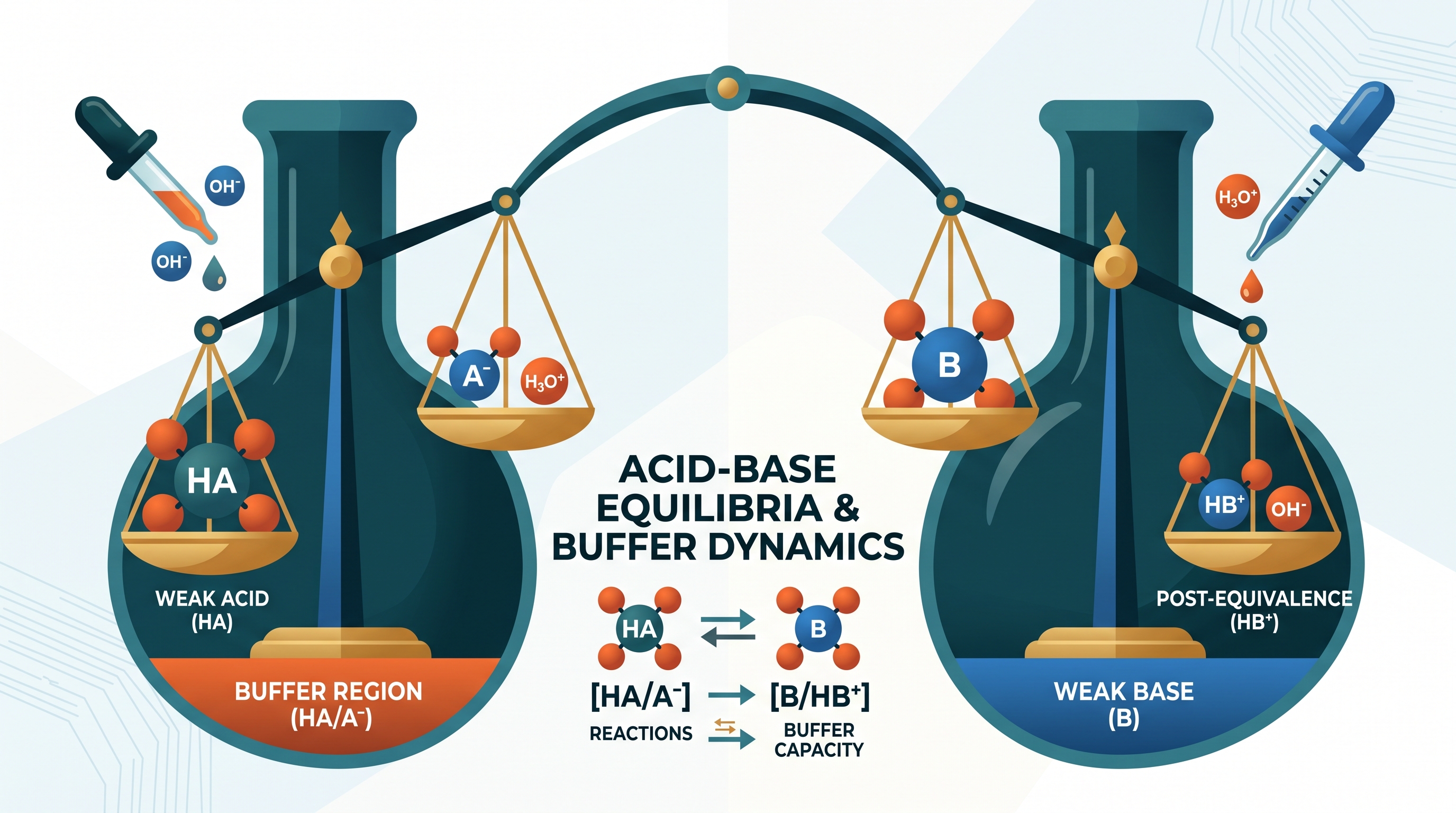
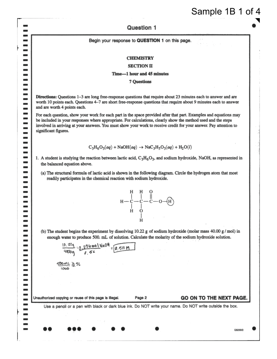
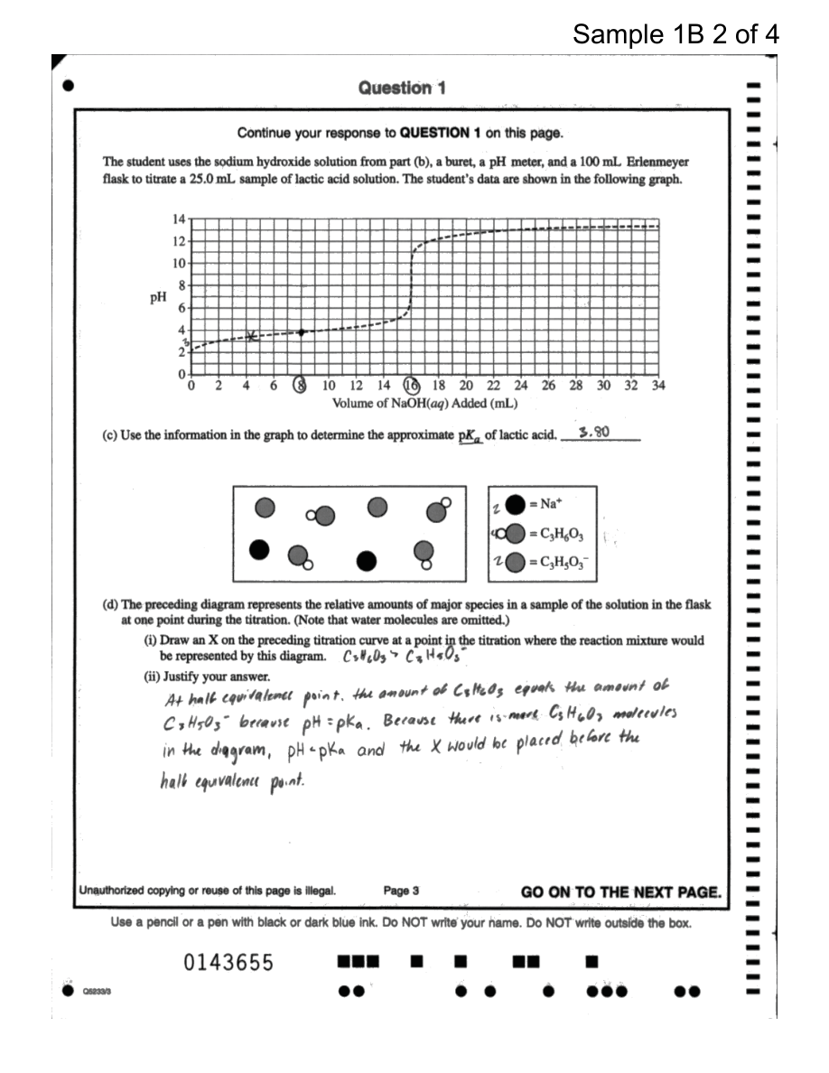
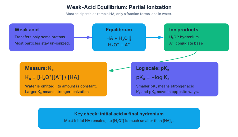
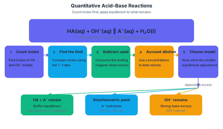
8.5 Acid-Base Titrations · 8.6 Molecular Structure of Acids and Bases
Key concepts: Acid-base reactions in aqueous solution and the role of water · Acid-base titrations of monoprotic and polyprotic acids or bases · Partial ionization and dynamic equilibrium of weak acids and bases · Hydronium and hydroxide concentrations in weak-acid and weak-base equilibria · Conjugate-base stabilization and its effect on acid strength · Electronegativity, inductive effects, and resonance in acid strength · Strong acids and their weak conjugate bases · Resonance stabilization of carboxylate ions
An acid-base titration determines an unknown concentration by measuring how much solution of known concentration is required to react with it. The same chemistry also explains why one molecule donates a proton readily while another barely ionizes: acid strength depends on the stability of the conjugate base left…
8.5 Acid-Base Titrations · 8.6 Molecular Structure of Acids and Bases
An acid-base titration determines an unknown concentration by measuring how much solution of known concentration is required to react with it. The same chemistry also explains why one molecule donates a proton readily while another barely ionizes: acid strength depends on the stability of the conjugate base left behind.
8.5 Acid-Base Titrations
A titration is best pictured as controlled chemical bookkeeping. A buret delivers a known amount of one reactant into a flask containing an unknown amount of another until the reacting species have been supplied in the exact stoichiometric ratio.
At the equivalence point, the moles of acid and base have reacted according to the balanced equation. The equivalence point is not automatically the same as the point where an indicator changes color; the indicator’s endpoint is an experimental signal chosen to occur very near equivalence.
For a monoprotic acid reacting with hydroxide,
$$ HA(aq)+OH^-(aq)\rightarrow A^-(aq)+H_2O(l) $$
the mole relationship is $1:1$. Therefore,
$$n_{HA}=n_{OH^-}$$
If a $0.1000\ \mathrm{M}$ sodium hydroxide solution requires $18.60\ \mathrm{mL}$ to reach the equivalence point when titrating $25.00\ \mathrm{mL}$ of an acid solution, then
$$n_{OH^-}=(0.1000\ \mathrm{mol,L^{-1}})(0.01860\ \mathrm{L})=1.860\times10^{-3}\ \mathrm{mol}$$
Because the acid is monoprotic, $n_{HA}=1.860\times10^{-3}\ \mathrm{mol}$. Its concentration is
$$[HA]=\frac{1.860\times10^{-3}\ \mathrm{mol}}{0.02500\ \mathrm{L}}=0.07440\ \mathrm{M}$$
For a polyprotic acid, one molecule can donate more than one proton. For example, complete neutralization of sulfuric acid can be represented overall as
$$ H_2SO_4(aq)+2OH^-(aq)\rightarrow SO_4^{2-}(aq)+2H_2O(l) $$
Thus, at complete neutralization, one mole of $H_2SO_4$ corresponds to two moles of $OH^-$. The balanced equation—not the volume alone—determines the mole ratio. Polyprotic titration curves can show more than one equivalence region when the successive proton-donation steps are sufficiently separated.
The species present at each stage control the solution’s properties. Before equivalence, excess acid may determine the hydronium concentration; at equivalence, the conjugate base or conjugate acid may react with water; after equivalence, excess strong titrant usually dominates the pH. A weak acid’s equivalence solution is often basic because its conjugate base reacts with water to form $OH^-$, whereas a weak base titrated with strong acid can produce an acidic equivalence solution because its conjugate acid forms $H_3O^+$.
Misconception check: Equivalence does not mean “the solution has pH $7.00$.” Neutral pH at equivalence is characteristic of a strong-acid/strong-base combination at approximately $25^\circ\mathrm{C}$, not a universal rule.
For weak acid–weak base titrations, the reaction may not proceed essentially to completion. Instead, the acid and base can establish an equilibrium, so interpretation must identify the reacting and remaining species rather than blindly applying a strong-neutralization shortcut.
8.6 Molecular Structure of Acids and Bases
Learning Objective 8.6.A: Explain the relationship between the strength of an acid or base and the structure of the molecule or ion.
Essential Knowledge 8.6.A.1: The protons on a molecule that will participate in acid-base reactions, and the relative strength of these protons, can be inferred from molecular structure. The central question is simple: after a proton leaves, how stable is the conjugate base?
A strong acid has a very weak conjugate base. In water, strong acids such as $HCl$, $HBr$, $HI$, $HClO_4$, $H_2SO_4$, and $HNO_3$ transfer protons readily because their conjugate bases are strongly stabilized by electronegativity, inductive effects, resonance, or a combination of these factors.
Electronegativity describes how strongly an atom attracts bonding electrons. If the negative charge of a conjugate base is located on a more electronegative atom, that charge is generally stabilized more effectively. For example, an electronegative halogen can support negative charge after the hydrogen in a hydrogen halide is removed.
An inductive effect is an electron-withdrawing or electron-donating influence transmitted through single bonds. Electronegative atoms near an acidic proton pull electron density away from the conjugate base, reducing the concentration of negative charge and increasing acid strength. The effect weakens as the electronegative atom becomes farther from the acidic site.
Resonance stabilization spreads charge over multiple atoms rather than confining it to one location. This is especially important for carboxylate ions. When a carboxylic acid loses its proton,
RCOOH\rightleftharpoons H^+ + RCOO^-
the negative charge in $RCOO^-$ is delocalized across both oxygen atoms. The two major resonance contributors give the two carbon–oxygen bonds equivalent character, making the conjugate base unusually stable for a weak acid. Carboxylic acids are therefore a common class of weak acids.
Common weak bases include nitrogenous bases such as ammonia and carboxylate ions. Strong bases, including group I and group II hydroxides, have very weak conjugate acids. In every case, basicity reflects the ion’s ability to accept a proton, while acid strength reflects the stability gained when the proton is removed.
AP Science Practices in Context
This topic most directly engages Science Practice 1: Models and Representations—especially 1.A: Describe and explain chemical representations and 1.B: Represent chemical phenomena using models—when students connect a titration curve, particle diagram, Lewis structure, and net ionic equation.
It also uses Science Practice 5: Mathematical Routines, including 5.A: Identify and describe the mathematical routines required to solve a problem and 5.B: Apply mathematical routines to solve problems, for mole ratios, molarity, and total-volume calculations. Science Practice 6: Argumentation, particularly 6.A: Make a claim and 6.B: Support a claim with evidence and reasoning, appears when students justify why resonance or electronegativity changes acid strength.
Retrieval check: A weak base has an initial concentration of $0.200\ \mathrm{M}$. Is $[OH^-]$ necessarily $0.200\ \mathrm{M}$? Explain. Then compare the conjugate bases of two acids: the acid whose conjugate base is more stabilized will be the stronger acid, because proton loss is more favorable.
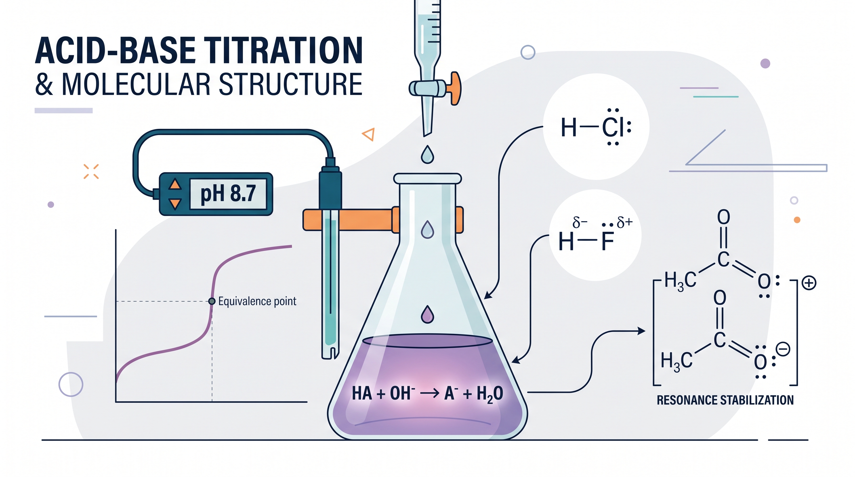
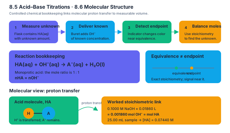
8.7 pH and pKₐ · 8.8 Properties of Buffers
Key concepts: pH · pKₐ · Properties of buffers
A buffer can absorb a small dose of acid or base while keeping its pH nearly steady because it contains a weak acid and the base formed when that acid loses a proton.
8.7 pH and pKₐ · 8.8 Properties of Buffers
A buffer can absorb a small dose of acid or base while keeping its pH nearly steady because it contains a weak acid and the base formed when that acid loses a proton. The key question is not simply how much acid is present, but how strongly the acid holds its proton and how much of each conjugate partner is available.
pH measures hydronium concentration
pH is a logarithmic measure of hydronium-ion concentration:
$$ \mathrm{pH}=-\log[H_3O^+] $$
A tenfold increase in $[H_3O^+]$ lowers the pH by exactly $1$ unit. Thus, a solution with $[H_3O^+]=1.0\times10^{-3}\ \mathrm{M}$ has $\mathrm{pH}=3.00$, while one with $[H_3O^+]=1.0\times10^{-5}\ \mathrm{M}$ has $\mathrm{pH}=5.00$. The second solution is one hundred times less concentrated in hydronium, not merely “two pH units less acidic.”
For a conjugate acid-base pair,
HA \rightleftharpoons H^+ + A^-
the acid-dissociation constant is
$$ K_a=\frac{[H_3O^+][A^-]}{[HA]} $$
where $HA$ is the weak acid and $A^-$ is its conjugate base. A larger $K_a$ means greater ionization and therefore a stronger acid.
pKₐ compares acid strength
pKₐ is the negative logarithm of $K_a$:
$$ \mathrm{p}K_a=-\log K_a $$
Because of the negative sign, smaller pKₐ values correspond to stronger acids. A difference of $2.60$ pKₐ units represents a factor of
$$ 10^{2.60}\approx 4.0\times10^2 $$
in $K_a$.
Consider two weak acids:
| Acid | pKₐ | Relative strength |
|---|---|---|
| $HA_1$ | $3.20$ | Stronger |
| $HA_2$ | $5.80$ | Weaker |
The acid with $\mathrm{p}K_a=3.20$ has the larger $K_a$ and ionizes more extensively. The difference is not a small numerical distinction: $HA_1$ is approximately $400$ times stronger than $HA_2$ because
$$ \frac{K_{a,1}}{K_{a,2}}=10^{5.80-3.20}=10^{2.60}\approx400 $$
Why a weak acid and its conjugate base make a buffer
A buffer requires appreciable amounts of both members of a conjugate pair, such as $HA/A^-$. The weak acid consumes added hydroxide:
$$ HA+OH^-\rightarrow A^-+H_2O $$
The conjugate base consumes added hydronium:
$$ A^-+H_3O^+\rightarrow HA+H_2O $$
These reactions remove most of the added strong base or strong acid before it can cause a large change in $[H_3O^+]$. The buffer does not make the pH perfectly constant; it makes the change smaller.
A buffer containing only $HA$ cannot efficiently remove added $H_3O^+$ because it lacks enough $A^-$. A solution containing only $A^-$ cannot efficiently remove added $OH^-$ because it lacks enough $HA$. The pair is essential.
pH, pKₐ, and the balance between buffer components
The pH of a weak-acid buffer depends strongly on the ratio of conjugate base to weak acid. When the concentrations of $HA$ and $A^-$ are equal, the acid equilibrium expression gives
$$ K_a=[H_3O^+] $$
so
$$ \mathrm{pH}=\mathrm{p}K_a $$
This is a special condition, not a universal identity. A solution’s pH equals its pKₐ only when the relevant weak acid and conjugate base are present in equal amounts.
A useful visual model is a proton-transfer balance:
$$ \begin{array}{c} \text{mostly }HA \quad \longleftrightarrow \quad \text{mostly }A^-\ \text{more capacity for }OH^- \qquad \text{more capacity for }H_3O^+ \end{array} $$
A buffer works best near its pKₐ because neither component is nearly depleted. If the solution contains overwhelmingly $HA$, it may neutralize added $OH^-$ but has little $A^-$ available for added acid. If it contains overwhelmingly $A^-$, the reverse limitation applies.
Worked comparison: choosing a buffer
Suppose a process must remain near pH $3.2$. Two candidate weak-acid systems have pKₐ values of $3.20$ and $5.80$.
- The $HA_1/A_1^-$ system has $\mathrm{p}K_a=3.20$, matching the target pH. Equal amounts of $HA_1$ and $A_1^-$ can therefore establish that pH and provide substantial resistance in both directions.
- The $HA_2/A_2^-$ system has $\mathrm{p}K_a=5.80$. At pH $3.2$, equilibrium strongly favors $HA_2$, leaving too little $A_2^-$ for effective removal of added $H_3O^+$.
- The first system is the better buffer for pH $3.2$.
Misconception check — “A stronger acid makes a better buffer.” A strong acid is highly ionized and does not coexist in useful equilibrium with a substantial conjugate-base concentration. Effective buffers generally use a weak acid and its conjugate base, with a pKₐ close to the desired pH.
AP reasoning in the chemistry
This topic uses Science Practice 1: Models and Representations when the equilibrium equation and conjugate-pair diagram represent particle-level proton transfer. It uses Science Practice 3: Representing Data and Phenomena when pH or pKₐ values are interpreted on a logarithmic scale, Science Practice 4: Model Analysis when a proposed buffer is judged from its component ratio, Science Practice 5: Mathematical Routines when logarithms and $K_a$ relationships are calculated, and Science Practice 6: Argumentation when buffer choice is justified with equilibrium evidence. Science Practice 2: Question and Method enters when an investigation tests how added acid or base changes a buffer’s pH.
Retrieval check: Two buffers have equal total concentration. Buffer $X$ uses an acid with $\mathrm{p}K_a=4.75$; buffer $Y$ uses an acid with $\mathrm{p}K_a=7.20$. For a target pH of $4.8$, which is better, and why? Buffer $X$: its pKₐ is close to the target, so both $HA$ and $A^-$ can remain available to neutralize additions of either $H_3O^+$ or $OH^-$.
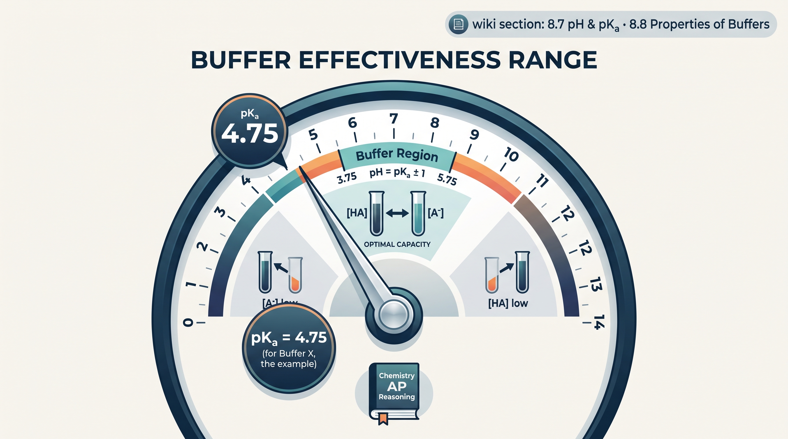
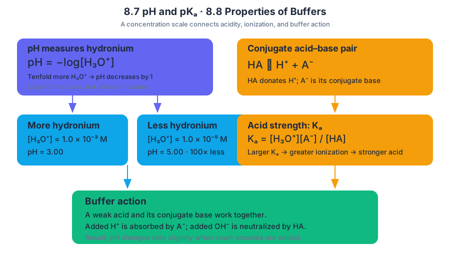
8.9 Henderson-Hasselbalch Equation · 8.10 Buffer Capacity
Key concepts: Henderson–Hasselbalch equation · Using the acid/conjugate-base concentration ratio to calculate pH · Determining pKa from the half-equivalence point · Interpreting titration curves · Identifying the buffer region · Recognizing the equivalence point · Calculating moles and molarity from titration data · Buffer capacity and the effect of buffer components
A buffer’s pH is controlled mainly by the ratio of conjugate base to weak acid, not by the absolute amount of solution. For a weak acid $\mathrm{HA}$ and its conjugate base $\mathrm{A^-}$:
8.9 Henderson–Hasselbalch Equation · 8.10 Buffer Capacity
A buffer’s pH is controlled mainly by the ratio of conjugate base to weak acid, not by the absolute amount of solution. For a weak acid $\mathrm{HA}$ and its conjugate base $\mathrm{A^-}$:
$$\mathrm{pH}=\mathrm{p}K_a+\log\left(\frac{[\mathrm{A^-}]}{[\mathrm{HA}]}\right)$$
Here, $[\mathrm{A^-}]$ is the concentration of the conjugate base and $[\mathrm{HA}]$ is the concentration of the weak acid. If both concentrations are multiplied or divided by the same factor, their ratio remains unchanged, so the pH remains approximately unchanged.
Using a concentration ratio to calculate pH
Suppose a buffer contains $0.020\ \mathrm{M}$ conjugate base and $0.010\ \mathrm{M}$ weak acid, with $\mathrm{p}K_a=4.1$. The ratio must be written in the order base over acid:
$$ \mathrm{pH}=4.1+\log\left(\frac{0.020}{0.010}\right) $$
$$ \mathrm{pH}=4.1+\log(2) $$
$$ \boxed{\mathrm{pH}\approx 4.4} $$
The base concentration is twice the acid concentration, so the logarithm is positive and the pH is higher than $\mathrm{p}K_a$. If the concentrations had been reversed, the ratio would be $0.5$, the logarithm would be negative, and the pH would be lower than $\mathrm{p}K_a$.
The half-equivalence point reveals $\mathrm{p}K_a$
During the titration of a weak acid with a strong base, the strong base converts some $\mathrm{HA}$ into $\mathrm{A^-}$:
$$ \mathrm{HA(aq)+OH^-(aq)\rightarrow A^-(aq)+H_2O(l)} $$
At the half-equivalence point, exactly half of the original weak acid has been neutralized. The moles of weak acid remaining equal the moles of conjugate base produced:
$$ [\mathrm{A^-}]=[\mathrm{HA}] $$
Therefore,
$$ \mathrm{pH}=\mathrm{p}K_a+\log(1)=\mathrm{p}K_a $$
For the $\mathrm{HAsc}$ titration, the equivalence point occurs at approximately $16.0\ \mathrm{mL}$ of $\mathrm{NaOH}$. The half-equivalence point is therefore $8.0\ \mathrm{mL}$, where the titration curve gives $\mathrm{pH}\approx 4.2$. The experimental value is reported as:
$$ \boxed{\mathrm{p}K_a\approx 4.1} $$
An acceptable experimental range is $4.0$–$4.3$. The equivalence-point pH, approximately $8.5$, is not the $\mathrm{p}K_a$.
Reading the titration curve
A weak-acid/strong-base titration curve has three visually important regions:
| Curve feature | Chemical meaning |
|---|---|
| Gentle rising region before equivalence | Buffer region: both $\mathrm{HA}$ and $\mathrm{A^-}$ are present |
| Midpoint of the steep rise | Equivalence point: stoichiometric neutralization is complete |
| Region after equivalence | Excess $\mathrm{OH^-}$ controls the pH |
For $\mathrm{HAsc}$, the buffer region includes $8.0\ \mathrm{mL}$ of added $\mathrm{NaOH}$, where $\mathrm{pH}\approx 4.2$. The sharp rise is centered near $16.0\ \mathrm{mL}$ and $\mathrm{pH}\approx 8.5$. The equivalence point is above $\mathrm{pH}=7$ because $\mathrm{Asc^-}$, the conjugate base of a weak acid, reacts with water to produce some $\mathrm{OH^-}$.
Connecting titration stoichiometry to buffer composition
At the equivalence point, the $1:1$ reaction means that the moles of $\mathrm{NaOH}$ added equal the original moles of $\mathrm{HAsc}$:
$$ 0.0160\ \mathrm{L}\times 0.0550\ \mathrm{mol\ L^{-1}} =8.80\times10^{-4}\ \mathrm{mol\ HAsc} $$
If the original acid sample volume was $0.0100\ \mathrm{L}$, its molarity was:
$$ [\mathrm{HAsc}] =\frac{8.80\times10^{-4}\ \mathrm{mol}}{0.0100\ \mathrm{L}} =\boxed{0.0880\ \mathrm{M}} $$
Before equivalence, added $\mathrm{OH^-}$ determines how much $\mathrm{HAsc}$ becomes $\mathrm{Asc^-}$. Those stoichiometric mole amounts can be used in the Henderson–Hasselbalch ratio because both species occupy the same solution volume; the volume factors cancel in the ratio.
Working backward from pH to the ratio
For a buffer with $\mathrm{pH}=4.7$ and $\mathrm{p}K_a=4.1$:
$$ 4.7=4.1+\log\left(\frac{[\mathrm{Asc^-}]}{[\mathrm{HAsc}]}\right) $$
$$ 0.6=\log\left(\frac{[\mathrm{Asc^-}]}{[\mathrm{HAsc}]}\right) $$
$$ \frac{[\mathrm{Asc^-}]}{[\mathrm{HAsc}]}=10^{0.6}\approx\boxed{4.0} $$
The expression $10^{-\mathrm{pH}}$ calculates $[\mathrm{H^+}]$. It does not calculate the buffer ratio. The ratio here requires $10^{\mathrm{pH}-\mathrm{p}K_a}$, so $10^{-(\mathrm{pH}-\mathrm{p}K_a)}$ gives the reciprocal ratio, not $\dfrac{[\mathrm{Asc^-}]}{[\mathrm{HAsc}]}$.
Buffer capacity
Buffer capacity is a buffer’s ability to resist a pH change when acid or base is added. Capacity depends on the amounts and relative proportions of both buffer components: $\mathrm{HA}$ must absorb added $\mathrm{OH^-}$, while $\mathrm{A^-}$ must absorb added $\mathrm{H^+}$.
A buffer has its greatest practical resistance near the half-equivalence point, where $[\mathrm{A^-}]=[\mathrm{HA}]$ and $\mathrm{pH}\approx\mathrm{p}K_a$. A very dilute buffer may have the correct pH but low capacity because only a small number of moles can react.
Misconception check: Equal pH does not necessarily mean equal buffer capacity. Two buffers can have the same base-to-acid ratio, and therefore the same pH, while the more concentrated buffer resists added acid or base more effectively.
These calculations exercise Science Practice 3: Representing Data and Phenomena, especially when extracting the half-equivalence and equivalence points from a curve; Science Practice 5: Mathematical Routines, when manipulating logarithms, ratios, and titration quantities; and Science Practice 6: Argumentation, when defending why a point on the curve represents $\mathrm{p}K_a$ or why a buffer resists pH change.
Retrieval check: A buffer has $\mathrm{p}K_a=5.0$, $[\mathrm{A^-}]=0.0010\ \mathrm{M}$, and $[\mathrm{HA}]=0.010\ \mathrm{M}$. Is its pH above or below $5.0$? Since $\dfrac{[\mathrm{A^-}]}{[\mathrm{HA}]}=0.10$, $\log(0.10)=-1$, so $\mathrm{pH}=4.0$, below $\mathrm{p}K_a$.
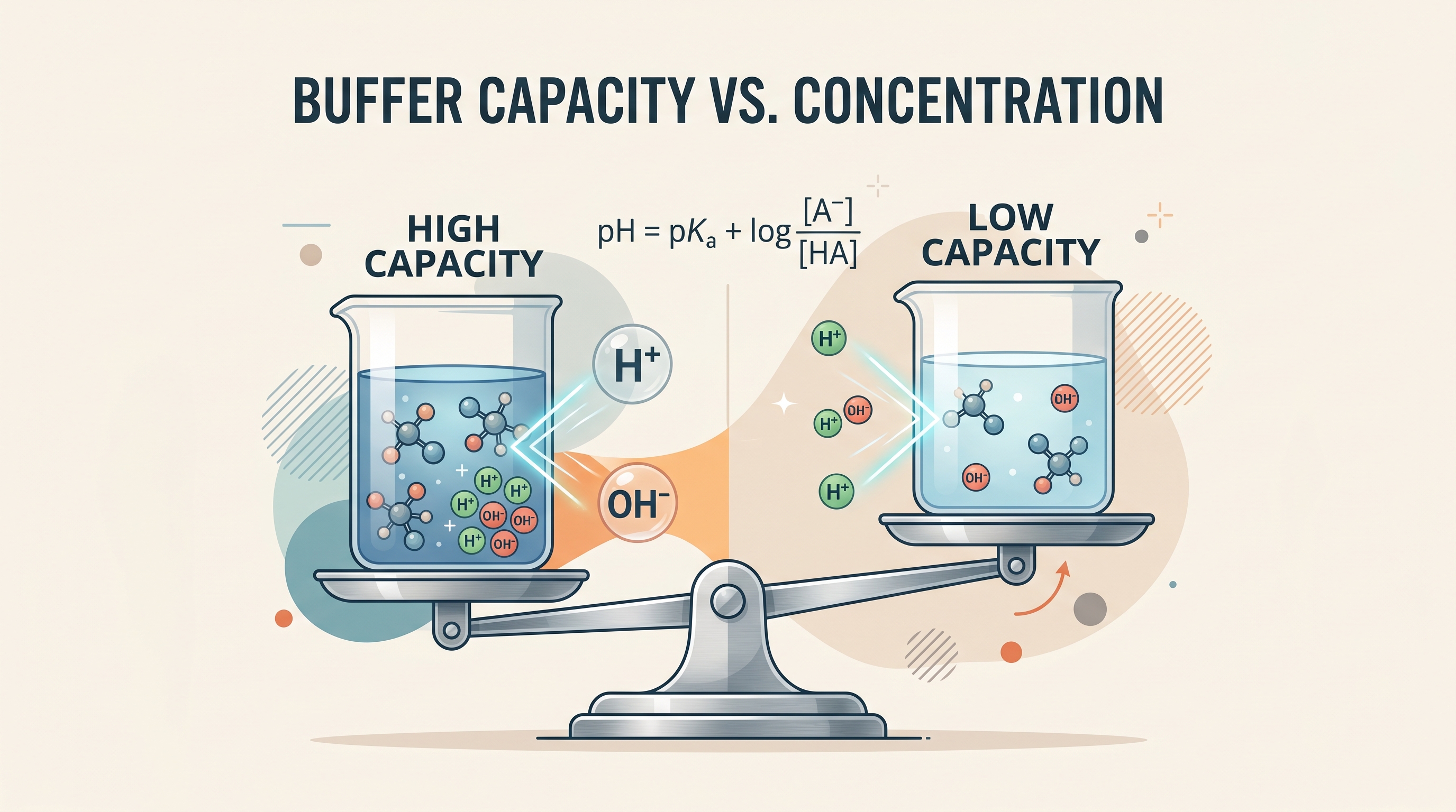
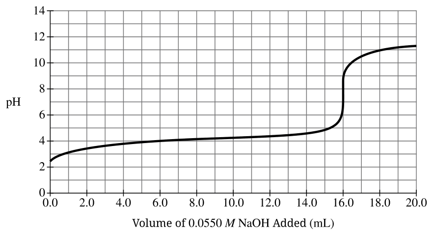
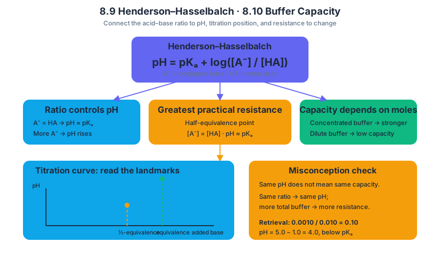
8.11 pH and Solubility
A solid can become more soluble simply because the solution contains acid or base. The key is that pH changes the concentration of ions already involved in a solubility equilibrium, pulling the equilibrium toward additional dissolving.
8.11 pH and Solubility
A solid can become more soluble simply because the solution contains acid or base. The key is that pH changes the concentration of ions already involved in a solubility equilibrium, pulling the equilibrium toward additional dissolving.
The central connection: acid–base chemistry shifts solubility
Solubility is the amount of a substance that dissolves to establish equilibrium with its undissolved solid. For a slightly soluble hydroxide such as magnesium hydroxide, the equilibrium is
$$ \mathrm{Mg(OH)_2(s) \rightleftharpoons Mg^{2+}(aq) + 2OH^-(aq)} $$
and its solubility-product expression is
$$ K_{sp}=[\mathrm{Mg^{2+}}][\mathrm{OH^-}]^2. $$
Adding acid removes hydroxide ions through neutralization:
$$ \mathrm{H^+(aq)+OH^-(aq)\rightarrow H_2O(l)} $$
Because the concentration of $\mathrm{OH^-}$ decreases, the ion product $Q_{sp}$ becomes smaller than $K_{sp}$. More $\mathrm{Mg(OH)_2}$ dissolves, producing additional $\mathrm{Mg^{2+}}$ and $\mathrm{OH^-}$ until equilibrium is restored. Thus, an acidic solution generally increases the solubility of a basic anion such as $\mathrm{OH^-}$.
Worked example: dissolving a metal hydroxide in acid
Suppose solid $\mathrm{Mg(OH)_2}$ is added to water containing hydrochloric acid. The process occurs in two linked steps:
- Dissolution:
$$ \mathrm{Mg(OH)_2(s)\rightleftharpoons Mg^{2+}(aq)+2OH^-(aq)} $$
- Neutralization:
$$ \mathrm{H^+(aq)+OH^-(aq)\rightarrow H_2O(l)} $$
Since $\mathrm{OH^-}$ is consumed, the dissolution equilibrium shifts right. The overall chemical result can be represented as
$$ \mathrm{Mg(OH)_2(s)+2H^+(aq)\rightarrow Mg^{2+}(aq)+2H_2O(l)}. $$
The solid is therefore more soluble at lower pH. Notice that acid does not change the numerical value of $K_{sp}$ at a fixed temperature; it changes the equilibrium position by removing one of the dissolved ions.
Which solids are affected by pH?
The same reasoning applies to salts containing basic anions. Anions such as $\mathrm{CO_3^{2-}}$, $\mathrm{S^{2-}}$, $\mathrm{F^-}$, and $\mathrm{OH^-}$ can react with $\mathrm{H^+}$. Removing these anions encourages more solid to dissolve.
For a carbonate solid,
$$ \mathrm{CaCO_3(s)\rightleftharpoons Ca^{2+}(aq)+CO_3^{2-}(aq)} $$
acid converts carbonate through reactions such as
$$ \mathrm{CO_3^{2-}(aq)+H^+(aq)\rightleftharpoons HCO_3^-(aq)} $$
and, with additional acid,
$$ \mathrm{HCO_3^-(aq)+H^+(aq)\rightarrow CO_2(g)+H_2O(l)}. $$
The formation of $\mathrm{CO_2(g)}$ can drive dissolution especially strongly because a product leaves the aqueous system.
Conversely, salts containing the conjugate bases of strong acids—such as $\mathrm{Cl^-}$, $\mathrm{NO_3^-}$, and $\mathrm{ClO_4^-}$—are not substantially protonated by ordinary acids. Their solubilities are therefore usually much less sensitive to pH.
| Solution condition | Ion removed or added | Typical effect on a basic-anion solid |
|---|---|---|
| Lower pH | $\mathrm{H^+}$ removes the basic anion | Solubility increases |
| Higher pH | Basic anion may accumulate | Solubility decreases |
| Near-neutral pH | Little protonation of the anion | $K_{sp}$ equilibrium dominates |
A particulate interpretation: saturated barium hydroxide
A saturated solution of barium hydroxide can be represented as
$$ \mathrm{Ba(OH)_2(s)\rightleftharpoons Ba^{2+}(aq)+2OH^-(aq)}. $$
If more $\mathrm{Ba(OH)2(s)}$ is added, the equilibrium concentrations do not change because the added material is a pure solid and does not appear in the $K{sp}$ expression. If water evaporates while solid remains present, more solid dissolves until the same saturation condition is reestablished. The pH remains essentially constant because the concentrations of $\mathrm{Ba^{2+}}$ and $\mathrm{OH^-}$ in the saturated solution return to their equilibrium values.
Misconception check
Misconception: “Adding acid always decreases solubility because it adds more particles.” The relevant question is not the total number of particles; it is whether the added $\mathrm{H^+}$ reacts with an ion in the solubility equilibrium. Acid increases the solubility of $\mathrm{Mg(OH)_2}$ because it removes $\mathrm{OH^-}$, but it has little direct effect on a chloride salt because $\mathrm{Cl^-}$ is the conjugate base of a strong acid.
CED alignment: Topic 8.11 pH and Solubility; Learning Objective 8.11.A; Essential Knowledge 2.D.1. The principal assessed practice is Science Practice 3: Representing Data and Phenomena (SP 3): connect a particulate model, a solubility equilibrium, and the macroscopic observation that pH or dissolved amount changes.
Retrieval check
A saturated solution contains $\mathrm{Ag_2S(s)}$:
$$ \mathrm{Ag_2S(s)\rightleftharpoons 2Ag^+(aq)+S^{2-}(aq)}. $$
Would lowering the pH generally increase or decrease its solubility? Explain in one sentence using an equilibrium argument.
Answer: Lowering the pH increases solubility because $\mathrm{H^+}$ reacts with the basic ion $\mathrm{S^{2-}}$, reducing its concentration and shifting the dissolution equilibrium to the right.
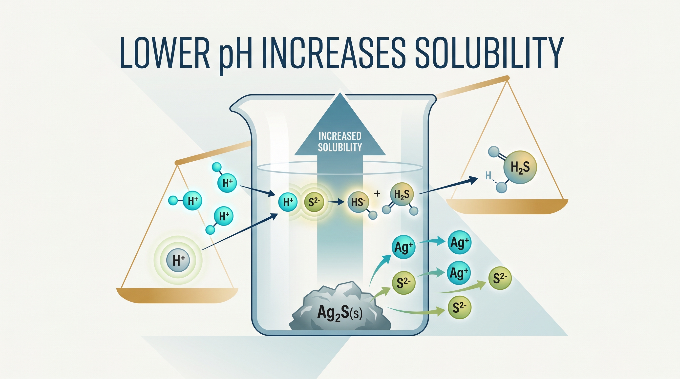
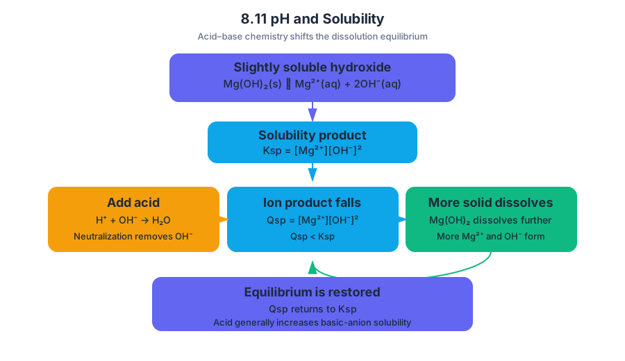
9.1 Introduction to Entropy · 9.2 Absolute Entropy and Entropy Change
Key concepts: Entropy · Introduction to entropy · Absolute entropy · Entropy change · Standard entropy change · Entropy change in chemical processes · Entropy change in physical processes · Temperature dependence of entropy · Calculating entropy change from absolute entropies · AP Chemistry science practice 6.C
Entropy measures how widely energy and matter can be distributed among the possible microscopic arrangements of a system. A warm gas in a large container has more possible molecular arrangements than a cool gas in a small container, so its entropy is greater.
9.1 Introduction to Entropy · 9.2 Absolute Entropy and Entropy Change
Entropy measures how widely energy and matter can be distributed among the possible microscopic arrangements of a system. A warm gas in a large container has more possible molecular arrangements than a cool gas in a small container, so its entropy is greater.
Investigative question: When a substance heats, melts, expands, or reacts, how can we predict whether its entropy increases or decreases—and calculate the change quantitatively?
Entropy as a particle-level idea
At the particulate level, entropy is connected to the number of available microstates, meaning the possible arrangements of particles and energy. More accessible arrangements correspond to greater entropy. This is why a gas generally has greater entropy than a liquid, and a liquid generally has greater entropy than a solid:
$$S_{\text{gas}} > S_{\text{liquid}} > S_{\text{solid}}$$
Heating also increases entropy. As temperature rises, particles occupy a broader range of energies and move through more possible arrangements. The change is not merely that particles “move faster”; the important point is that higher temperature makes more energy distributions accessible.
AP skill connection — 6.C: Support a claim with evidence from representations or models at the particulate level, such as the structure of atoms and/or molecules. To use 6.C, connect a macroscopic observation—such as melting or heating—to a particle-level model. For example, when ice melts, water molecules lose the rigid positional order of the crystal and can occupy many more arrangements in the liquid. That model supports the claim that $\Delta S > 0$.
9.1 Introduction to Entropy
The CED learning objective 9.1.A: Identify the sign and relative magnitude of the entropy change associated with chemical or physical processes. The symbol $\Delta S$ means entropy change, calculated as the final entropy minus the initial entropy:
$$\Delta S = S_{\text{final}} - S_{\text{initial}}$$
A positive entropy change, $\Delta S > 0$, indicates that the system has access to more arrangements after the process. A negative entropy change, $\Delta S < 0$, indicates fewer accessible arrangements. A phase change from liquid to gas, the expansion of a gas, or the production of more gas particles usually increases entropy.
For chemical reactions, compare the structures and physical states of the reactants and products. A reaction that produces more moles of gas particles generally has a larger positive entropy change than one that produces fewer gas particles. However, particle count is evidence—not an automatic rule: molecular complexity, phase, and the types of particles also matter.
Misconception check: “Entropy means disorder”
“Disorder” is a useful first image but an incomplete definition. Entropy is not a visual judgment about whether a sample looks messy; it concerns the number of microscopic arrangements available to the particles and energy. A neatly arranged gas can still have greater entropy than a disordered solid because gas particles have far more freedom to move.
9.2 Absolute entropy and entropy change
Absolute entropy is the entropy of a substance itself, not the change caused by a process. Standard molar entropy, written $S^\circ$, is the absolute entropy of $1$ mole of a substance under standard conditions, commonly reported in $\mathrm{J,mol^{-1},K^{-1}}$. Unlike enthalpy values that may be assigned relative zeros, absolute entropies can be used directly in reaction calculations.
The CED learning objective 9.2.A: Calculate the standard entropy change for a chemical or physical process based on the absolute entropies (standard molar entropies) of the species involved in the process. Its essential knowledge statement, 9.2.A.1, gives the central relationship:
$$\Delta S^\circ_{\text{reaction}}= \sum S^\circ_{\text{products}}- \sum S^\circ_{\text{reactants}}$$
The coefficients in the balanced equation multiply the standard molar entropy values. The units remain $\mathrm{J,mol^{-1},K^{-1}}$ for a reaction as written. Always subtract reactants from products; reversing that order changes the sign.
Worked example: a chemical process
Suppose a reaction as written has the following standard molar entropies:
$$ \mathrm{A(g)+2B(g)\rightarrow C(g)} $$
$$S^\circ_{\mathrm{A}}=190\ \mathrm{J,mol^{-1},K^{-1}}$$
$$S^\circ_{\mathrm{B}}=160\ \mathrm{J,mol^{-1},K^{-1}}$$
$$S^\circ_{\mathrm{C}}=250\ \mathrm{J,mol^{-1},K^{-1}}$$
Apply the products-minus-reactants pathway:
$$\Delta S^\circ= (1)(250)- \left[(1)(190)+(2)(160)\right]$$
$$\Delta S^\circ=250-510=-260\ \mathrm{J,mol^{-1},K^{-1}}$$
The negative result means the products have fewer accessible arrangements overall. The reaction changes three moles of gaseous particles into one mole of gaseous particles, providing a strong particle-level explanation for $\Delta S^\circ<0$.
Misconception check: absolute entropy is not entropy change
A substance can have a large positive absolute entropy, $S^\circ$, while participating in a process with a negative $\Delta S^\circ$. For example, the products may each have substantial entropy, yet their stoichiometric total can still be smaller than the reactants’ total. Never interpret the sign of an individual $S^\circ$ value as the sign of the process’s $\Delta S^\circ$.
Worked example: a physical process
For vaporization,
$$ \mathrm{H_2O(l)\rightarrow H_2O(g)} $$
if $S^\circ_{\mathrm{H_2O(l)}}=70.0\ \mathrm{J,mol^{-1},K^{-1}}$ and $S^\circ_{\mathrm{H_2O(g)}}=189.0\ \mathrm{J,mol^{-1},K^{-1}}$, then
$$\Delta S^\circ= 189.0-70.0= +119.0\ \mathrm{J,mol^{-1},K^{-1}}$$
The positive value matches the physical model: liquid water molecules become gas particles with much greater freedom of translation and many more accessible arrangements. The same calculation applies to melting, freezing, sublimation, condensation, and other physical processes; only the substances and states before and after the process change.
Exam-ready calculation pathway
AP skill connection — 5.F: Calculate, estimate, or predict an unknown quantity from known quantities by selecting and following a logical computational pathway and attending to precision (e.g., performing dimensional analysis and attending to significant figures). For a standard entropy calculation:
- Balance or write the process correctly, including physical states.
- Identify every product and reactant entropy value.
- Multiply each $S^\circ$ by its stoichiometric coefficient.
- Add the product terms.
- Add the reactant terms.
- Subtract products minus reactants.
- Report the sign, units, and appropriate precision.
Retrieval check: For $\mathrm{X(s)\rightarrow X(l)}$, would $\Delta S^\circ$ usually be positive or negative? Which term belongs first in the calculation: $S^\circ_{\mathrm{X(s)}}$ or $S^\circ_{\mathrm{X(l)}}$? The answer is positive, with the liquid term first:
$$\Delta S^\circ=S^\circ_{\mathrm{X(l)}}-S^\circ_{\mathrm{X(s)}}$$
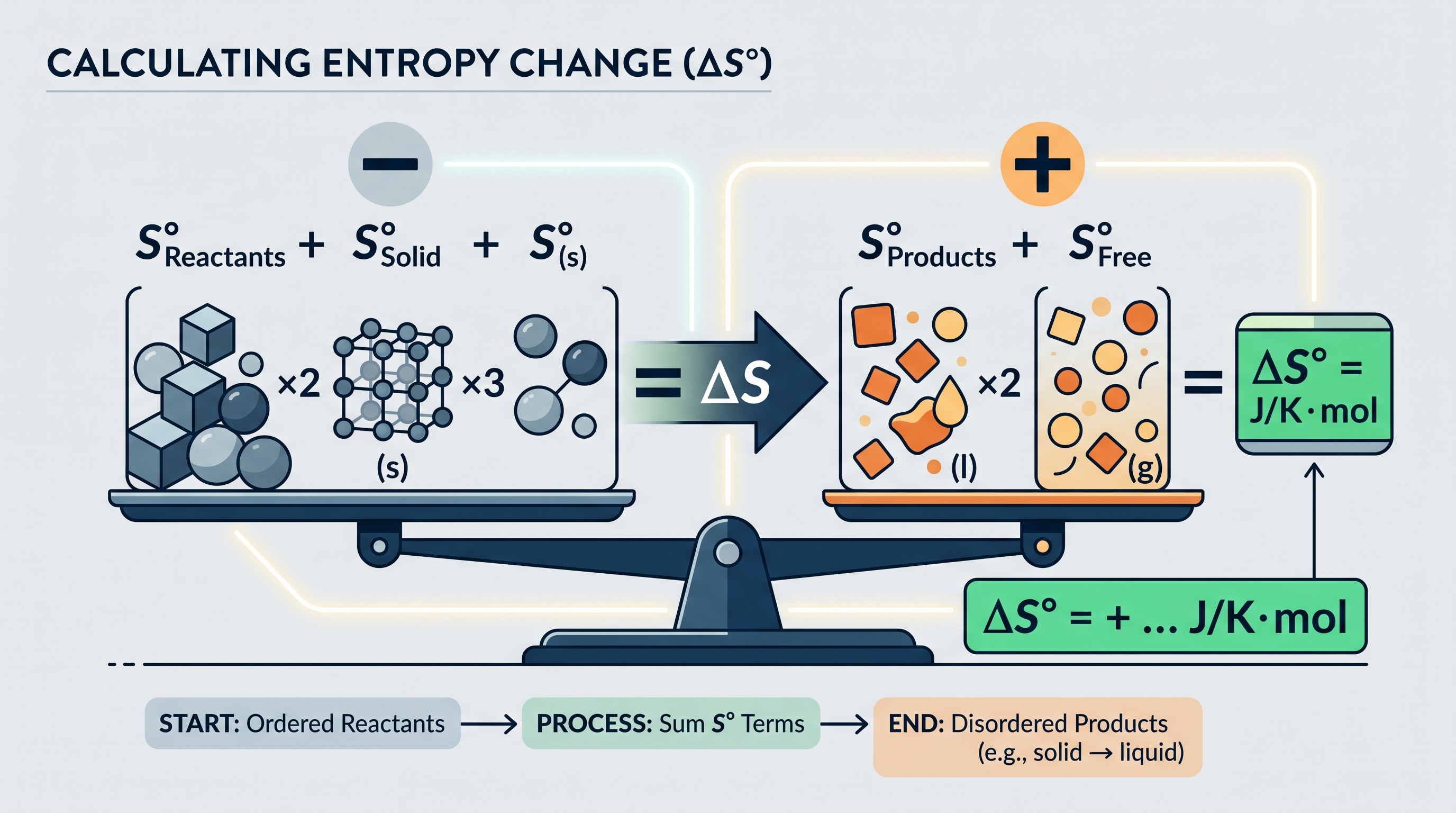
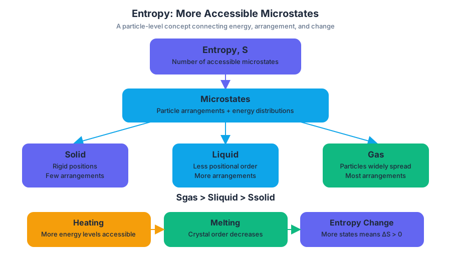
9.3 Gibbs Free Energy and Thermodynamic Favorability · 9.4 Thermodynamic and Kinetic Control
Key concepts: Gibbs free energy (ΔG°) · Thermodynamic favorability · The relationship between enthalpy, entropy, temperature, and free energy · Thermodynamic control · Kinetic control · Activation energy · Reaction rate · Chemical equilibrium · Distinguishing equilibrium from kinetic inhibition · The relationship between ΔG° and the equilibrium constant K
A reaction can be energetically favorable yet appear to do nothing: a thermodynamically favored process may be trapped behind a large activation-energy barrier. Gibbs free energy answers whether products are favored, while kinetics answers how quickly the system can get there.
9.3 Gibbs Free Energy and Thermodynamic Favorability · 9.4 Thermodynamic and Kinetic Control
A reaction can be energetically favorable yet appear to do nothing: a thermodynamically favored process may be trapped behind a large activation-energy barrier. Gibbs free energy answers whether products are favored, while kinetics answers how quickly the system can get there.
The free-energy test
Gibbs free energy combines enthalpy, entropy, and temperature into one quantity that predicts thermodynamic favorability:
$$\Delta G^\circ_{\mathrm{rxn}}=\Delta H^\circ_{\mathrm{rxn}}-T\Delta S^\circ_{\mathrm{rxn}}$$
Here, $T$ must be measured in kelvins, and $\Delta H^\circ$ and $\Delta S^\circ$ must use compatible energy units. A process is thermodynamically favored under the stated conditions when $\Delta G^\circ_{\mathrm{rxn}}<0$.
Key distinction: $\Delta G^\circ<0$ means the process is thermodynamically favored; it does not mean the process is fast.
The signs of $\Delta H^\circ$ and $\Delta S^\circ$ determine whether temperature matters.
| $\Delta H^\circ$ | $\Delta S^\circ$ | Temperature effect | Favorability |
|---|---|---|---|
| $<0$ | $>0$ | Both terms make $\Delta G^\circ$ negative | Favored at all $T$ |
| $>0$ | $<0$ | Both terms make $\Delta G^\circ$ positive | Not favored at any $T$ |
| $>0$ | $>0$ | The $-T\Delta S^\circ$ term becomes more negative as $T$ rises | Favored at high $T$ |
| $<0$ | $<0$ | The $-T\Delta S^\circ$ term becomes more positive as $T$ rises | Favored at low $T$ |
Temperature as the deciding variable
When $\Delta H^\circ_{\mathrm{rxn}}>0$ and $\Delta S^\circ_{\mathrm{rxn}}>0$, the process is endothermic but produces a favorable entropy change. At sufficiently high temperature, the magnitude of $T\Delta S^\circ$ can exceed $\Delta H^\circ$, making $\Delta G^\circ$ negative.
Worked example. Suppose a process has $\Delta H^\circ_{\mathrm{rxn}}=+40.0\ \mathrm{kJ,mol^{-1}}$ and $\Delta S^\circ_{\mathrm{rxn}}=+100.\ \mathrm{J,mol^{-1},K^{-1}}$. Convert enthalpy to joules:
$$\Delta H^\circ_{\mathrm{rxn}}=+4.00\times10^4\ \mathrm{J,mol^{-1}}$$
At $500\ \mathrm{K}$:
$$\Delta G^\circ=(4.00\times10^4)-(500)(100.)=-1.00\times10^4\ \mathrm{J,mol^{-1}}$$
Because $\Delta G^\circ<0$, the process is thermodynamically favored at $500\ \mathrm{K}$. The crossover temperature occurs when $\Delta G^\circ=0$:
$$T=\frac{\Delta H^\circ}{\Delta S^\circ} =\frac{4.00\times10^4}{100.}=400\ \mathrm{K}$$
Thus, this process is favored above approximately $400\ \mathrm{K}$, assuming $\Delta H^\circ$ and $\Delta S^\circ$ remain constant.
Misconception check: A positive $\Delta S^\circ$ does not automatically make a reaction favored. The enthalpy term may still dominate at lower temperature.
Thermodynamic favorability and equilibrium tendency
The standard free energy and equilibrium constant are connected by
$$K=e^{-\Delta G^\circ/RT}$$
and equivalently
$$\Delta G^\circ=-RT\ln K$$
where $R$ is the gas constant and $T$ is the absolute temperature. If $\Delta G^\circ$ is near zero, $K$ is close to $1$; if $\left|\Delta G^\circ\right|$ is much larger than $RT$, $K$ deviates substantially from $1$.
A negative $\Delta G^\circ$ corresponds to $K>1$, so products are favored relative to reactants under standard conditions. A positive $\Delta G^\circ$ corresponds to $K<1$, so the process is not thermodynamically favored in the stated direction.
Thermodynamic control versus kinetic control
Thermodynamic control describes a situation in which the relative stability of products determines the observed outcome. The product arrangement with lower free energy is favored, provided the system can reach it.
Kinetic control occurs when a high activation-energy barrier prevents rapid conversion, even though the overall process has $\Delta G^\circ<0$. Activation energy, $E_a$, is the minimum energy required for reacting particles to reach the transition state.
A useful energy-profile comparison is:
- Thermodynamics: compare the energy of reactants and products; this determines $\Delta G$.
- Kinetics: compare the reactants with the transition state; this determines $E_a$ and strongly affects rate.
- Equilibrium: occurs when forward and reverse reaction rates are equal.
For example, carbon and oxygen can form carbon dioxide thermodynamically, but a piece of carbon does not instantly burst into flame in ordinary air. A spark supplies enough energy to overcome the activation barrier. Before ignition, the reaction is not necessarily at equilibrium; it may simply be kinetically inhibited.
Exam-critical distinction: Failure to observe a process at a noticeable rate does not prove that the system is at equilibrium. “Not visibly reacting” can mean “very slow,” not “forward and reverse rates are equal.”
AP Chemistry reasoning in this topic
Learning Objective 9.3.A: Explain whether a physical or chemical process is thermodynamically favored based on an evaluation of $\Delta G^\circ$. The essential knowledge is applied through the relationship $\Delta G^\circ=\Delta H^\circ-T\Delta S^\circ$, sign analysis, temperature reasoning, and the connection between $\Delta G^\circ$ and $K$ (EK 9.3.A.1–9.3.A.2).
Learning Objective 9.4.A: Explain the relationship between thermodynamic favorability and the rate at which a process occurs. The essential knowledge requires distinguishing a favorable process from a rapid process and relating kinetic inhibition to activation energy (EK 9.4.A.1–9.4.A.2).
The main science practices are Science Practice 1: Models and Representations when interpreting energy profiles, Science Practice 4: Model Analysis when connecting $\Delta H^\circ$, $\Delta S^\circ$, $\Delta G^\circ$, and $E_a$, Science Practice 5: Mathematical Routines when calculating free energy or $K$, and Science Practice 6: Argumentation when justifying favorability with an equation and a sign-based conclusion.
Retrieval check: A reaction has $\Delta H^\circ>0$ and $\Delta S^\circ>0$. Is it favored at all temperatures, no temperatures, low temperatures, or high temperatures? Explain using the sign of the $-T\Delta S^\circ$ term. Then state whether a measured rate of essentially zero proves equilibrium.
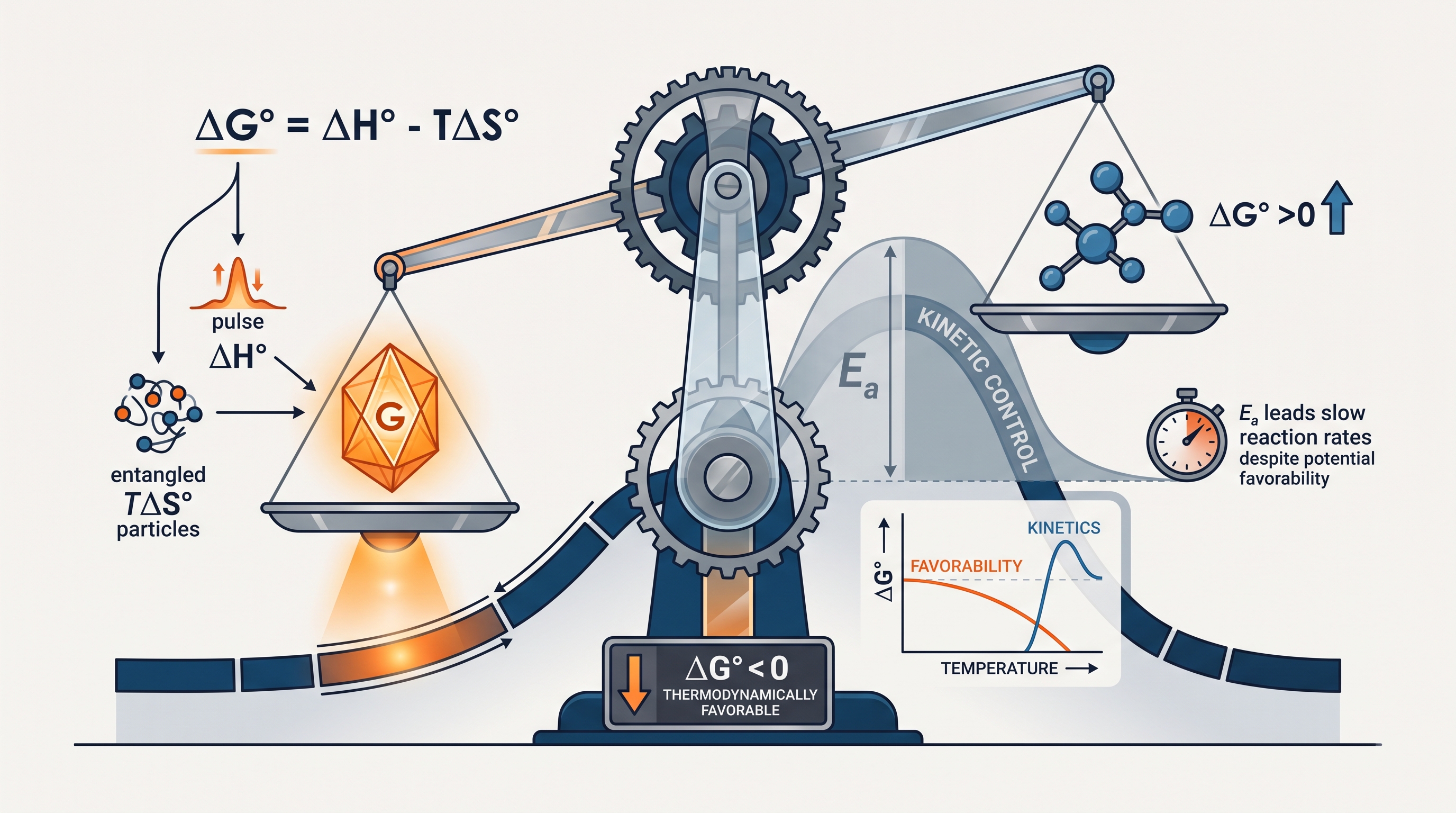
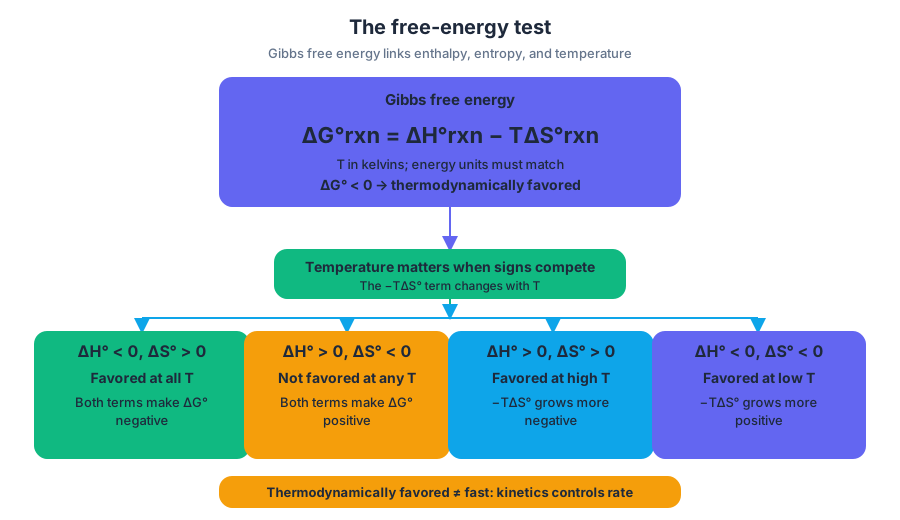
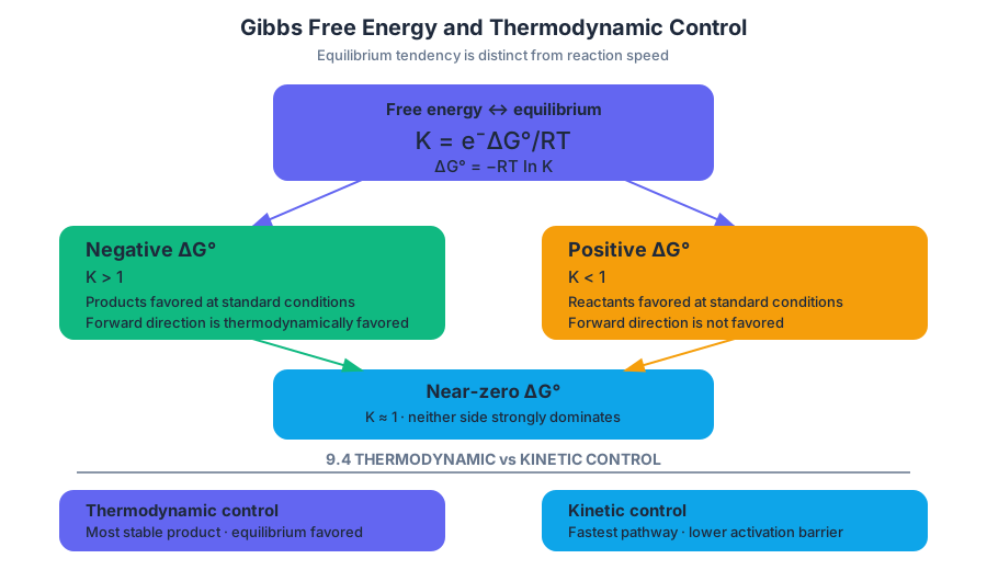
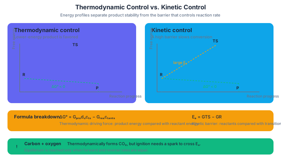
9.5 Free Energy and Equilibrium · 9.6 Free Energy of Dissolution
Key concepts: Gibbs free energy change (ΔG°) as a criterion for spontaneity and equilibrium · The relationship ΔG° = ΔH° − TΔS° · The relationship between ΔG° and the equilibrium constant K · How enthalpy and entropy changes affect the solubility of a salt · The three energetic factors in dissolution: breaking solute–solute interactions, breaking solvent–solvent interactions, and forming solute–solvent interactions · Why determining the total free-energy change of dissolution can be challenging because contributions may cancel · How favorable solvent–solute interactions influence dissolution · How changes in temperature can affect the free energy and solubility of a substance · Using calorimetry and temperature change to investigate the enthalpy of dissolution, such as dissolving KCl in water · The dissolution of magnesium hydroxide as an example of a sparingly soluble ionic compound
A salt can dissolve even when the solution becomes colder because spontaneity is controlled by free energy, not enthalpy alone. The decisive quantity is the standard free-energy change for dissolution, $\Delta G^\circ_{\mathrm{dissolution}}$: the Gibbs free-energy change when a specified amount of a substance…
9.5 Free Energy and Equilibrium · 9.6 Free Energy of Dissolution
A salt can dissolve even when the solution becomes colder because spontaneity is controlled by free energy, not enthalpy alone. The decisive quantity is the standard free-energy change for dissolution, $\Delta G^\circ_{\mathrm{dissolution}}$: the Gibbs free-energy change when a specified amount of a substance dissolves under standard conditions.
Key criterion: If $\Delta G^\circ_{\mathrm{dissolution}}<0$, dissolution is thermodynamically favorable under standard conditions; if $\Delta G^\circ_{\mathrm{dissolution}}>0$, the undissolved solid is favored under standard conditions.
The free-energy balance
Free energy combines two competing effects: enthalpy, the heat-related energy change, and entropy, the change associated with the distribution of energy and matter among possible microscopic arrangements. Their relationship is
$$ \Delta G^\circ=\Delta H^\circ-T\Delta S^\circ $$
where $\Delta H^\circ$ is the standard enthalpy change, $\Delta S^\circ$ is the standard entropy change, and $T$ is the absolute temperature in kelvins.
A negative $\Delta H^\circ$ favors dissolution because the process releases energy. A positive $\Delta S^\circ$ also favors dissolution because the dissolved particles may be distributed among more positions and arrangements. However, either contribution can dominate: a dissolution with $\Delta H^\circ>0$ may still be favorable if the entropy increase is sufficiently large, especially at higher temperature.
The temperature factor matters because $T\Delta S^\circ$ grows as temperature increases. Thus, the same enthalpy and entropy changes can produce different free-energy changes at different temperatures. Solubility therefore depends on the combined enthalpy and entropy changes of dissolution, not on whether dissolution is simply exothermic or endothermic.
Free energy and equilibrium
At equilibrium, the forward and reverse processes continue microscopically, but there is no net thermodynamic driving force. The actual free-energy change under the existing conditions is
$$ \Delta G=0 $$
The standard free-energy change is connected to the equilibrium constant by
$$ \Delta G^\circ=-RT\ln K $$
where $R$ is the gas constant, $T$ is temperature in kelvins, and $K$ is the equilibrium constant.
This equation gives a useful scale:
- $K>1$ means $\ln K>0$, so $\Delta G^\circ<0$ and products are favored under standard conditions.
- $K<1$ means $\ln K<0$, so $\Delta G^\circ>0$ and reactants are favored under standard conditions.
- $K=1$ means $\Delta G^\circ=0$.
The important distinction is that $\Delta G^\circ$ describes standard conditions, whereas $\Delta G$ describes the current mixture. At equilibrium, $\Delta G$ is zero even when $\Delta G^\circ$ is not.
Why dissolving a salt requires three energetic steps
The CED learning objective 9.6.A is to explain the relationship between salt solubility and the enthalpy and entropy changes occurring during dissolution. Essential knowledge 9.6.A.1 identifies three particulate-level contributions that determine $\Delta G^\circ_{\mathrm{dissolution}}$.
Imagine separating an ionic solid into hydrated ions. The process can be analyzed as a three-part energy accounting system:
- Breaking solute–solute interactions: Energy is required to pull ions or molecules out of the solid lattice. For an ionic crystal, this means overcoming strong electrostatic attractions.
- Disrupting solvent–solvent interactions: Solvent particles must move apart to create space. This also requires energy because attractive interactions within the solvent are being disturbed.
- Forming solute–solvent interactions: New attractions form between the dissolved particles and solvent molecules. These interactions may release energy, or in some cases require energy overall.
The total enthalpy and entropy changes result from all three steps.
Why solubility can be difficult to predict
Each step changes both energy and molecular organization. Separating a rigid crystal may increase the number of accessible arrangements, while reorganizing solvent molecules around ions can make the solvent locally more ordered. Hydration or solvation may release substantial energy, but it also creates structured shells around the dissolved particles.
Because the three contributions can have opposite signs, their free energies may partially cancel:
$$ \Delta G^\circ_{\mathrm{dissolution}}
\Delta G^\circ_{\mathrm{solute-solute}} + \Delta G^\circ_{\mathrm{solvent-solvent}} + \Delta G^\circ_{\mathrm{solute-solvent}} $$
The individual contributions may be estimated in sign and relative magnitude, but predicting the exact total can be challenging. A salt with an endothermic dissolution is not automatically insoluble, and a salt with an exothermic dissolution is not automatically highly soluble.
Named misconception — “Heat determines solubility.”
An endothermic dissolution can be favorable if the entropy term is sufficiently favorable. Solubility reflects the net $\Delta G$, not $\Delta H$ alone.
Evidence from potassium chloride
When potassium chloride, $KCl$, dissolves in water, the solution temperature decreases. Calorimetry interprets this temperature drop as evidence that the dissolution process absorbs heat from the surroundings:
$$ \Delta H_{\mathrm{dissolution}}>0 $$
This observation identifies the enthalpy contribution, but it does not by itself establish whether dissolution is thermodynamically favorable. The entropy change and the resulting $\Delta G$ must also be considered.
Magnesium hydroxide: equilibrium, not “no dissolving”
Magnesium hydroxide, $Mg(OH)_2$, is sparingly soluble, but its dissolution is an equilibrium process:
Mg(OH)_2(s)\rightleftharpoons Mg^{2+}(aq)+2OH^-(aq)
A small solubility means that equilibrium strongly favors the solid, corresponding to a small equilibrium constant for dissolution and therefore a positive or only weakly favorable $\Delta G^\circ$ under standard conditions. It does not mean that no particles dissolve.
For AP Skill 4.D, “Explain the degree to which a model or representation describes the connection between particulate-level properties and macroscopic properties,” connect the microscopic model to the observation: lattice attractions, solvent reorganization, and hydration determine the free-energy balance; that balance determines $K$; and $K$ determines the equilibrium extent of dissolution observed as solubility.
Retrieval check
A salt dissolves with $\Delta H^\circ>0$, but its solubility increases as temperature rises. What must be true about the entropy contribution over the relevant temperature range? Why would the temperature decrease during dissolution fail to prove that the salt is insoluble? A complete answer should identify a favorable $\Delta S^\circ$, apply $\Delta G^\circ=\Delta H^\circ-T\Delta S^\circ$, and distinguish enthalpy from the total free-energy change.
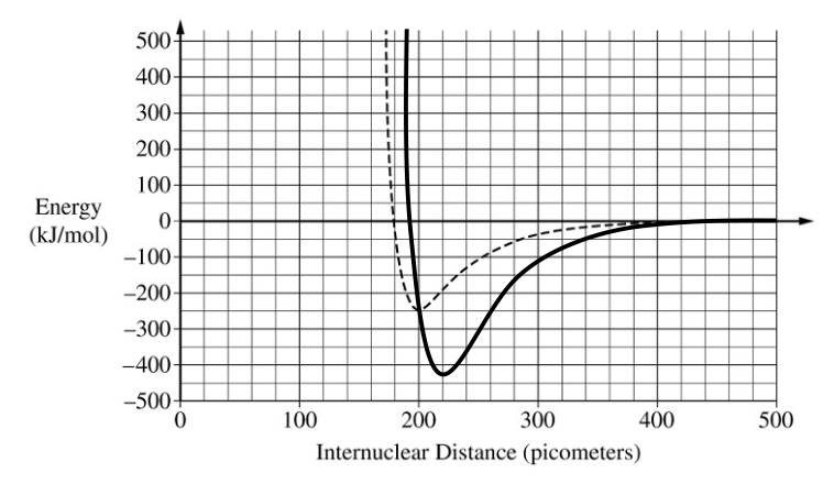
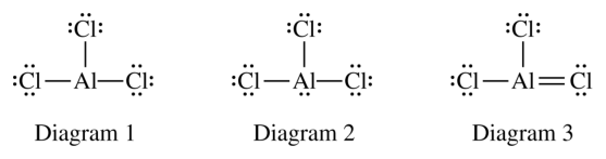
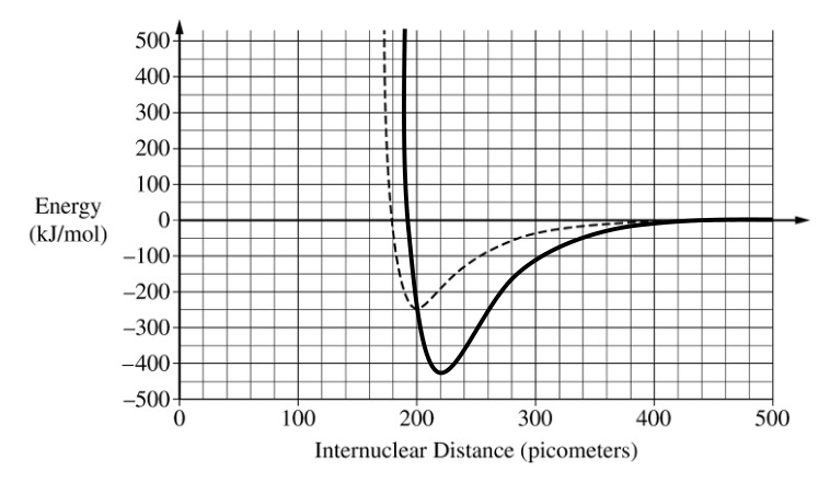
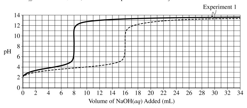
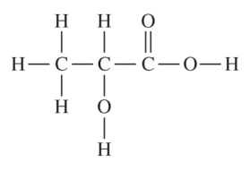
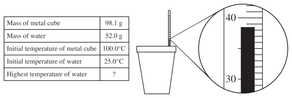
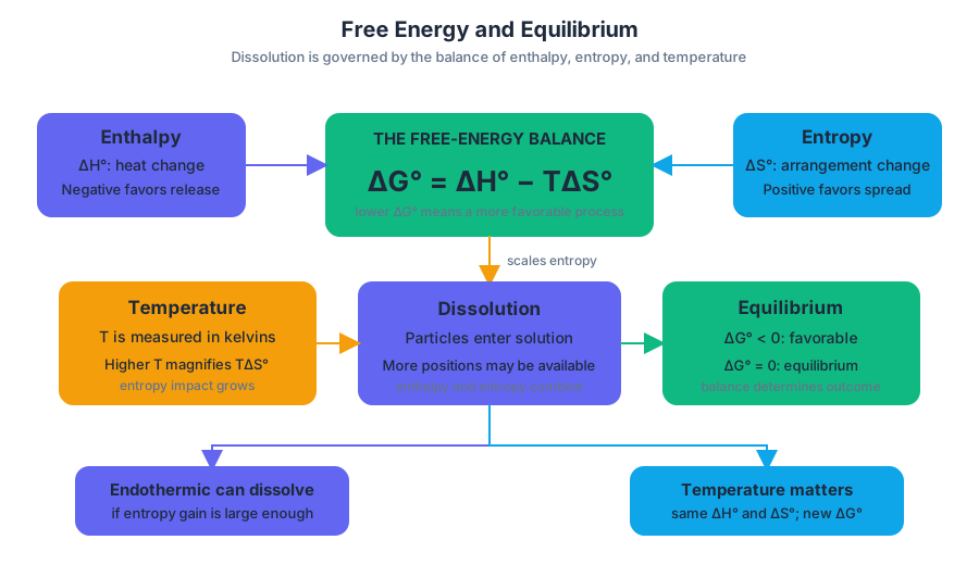
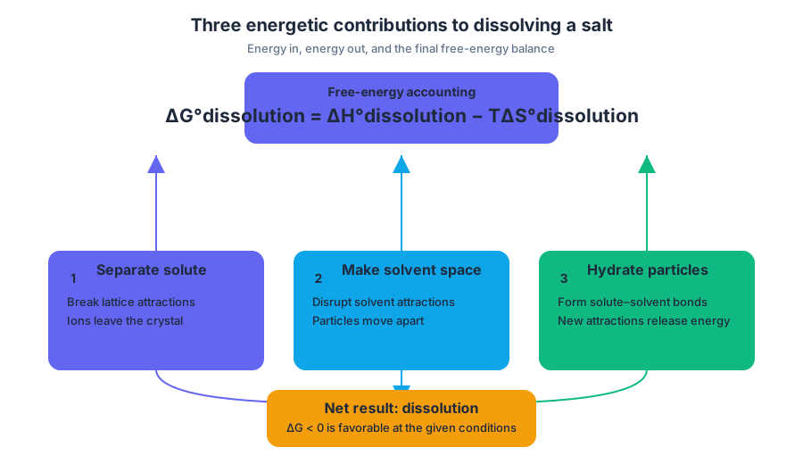
9.7 Coupled Reactions · 9.8 Galvanic (Voltaic) and Electrolytic Cells
Key concepts: Coupled reactions and using an external energy source to drive thermodynamically unfavorable processes · Galvanic ( voltaic) cells · Electrolytic cells · Physical components and operational principles of electrochemical cells · Roles of electrodes, half-cell solutions, salt bridges, and voltage/current measuring devices · Oxidation and reduction at electrodes · Identifying the anode and cathode from electrode mass changes · Standard reduction potentials and electrochemical cell voltage · Stoichiometric relationships governing electrode mass changes · Relating cell descriptions and half-reactions to overall cell behavior
A redox reaction can either release usable electrical energy or consume electrical energy to force an otherwise unfavorable chemical change. The difference is the direction of energy conversion: a galvanic cell converts chemical energy into electrical energy, while an electrolytic cell uses an external energy…
9.7 Coupled Reactions · 9.8 Galvanic (Voltaic) and Electrolytic Cells
A redox reaction can either release usable electrical energy or consume electrical energy to force an otherwise unfavorable chemical change. The difference is the direction of energy conversion: a galvanic cell converts chemical energy into electrical energy, while an electrolytic cell uses an external energy source to drive a thermodynamically unfavorable reaction.
Learning Objective 9.8.A: Explain the relationship between the physical components of an electrochemical cell and the overall operational principles of the cell.
Coupled reactions: chemical energy and electrical energy
A redox reaction contains two coupled half-reactions. Oxidation removes electrons from one species, and reduction adds those electrons to another species. Because electrons released by oxidation must be consumed by reduction, the two processes cannot operate independently: they are chemically coupled.
In a galvanic cell, the favorable redox reaction is separated into two half-cells. Electrons are forced to travel through an external wire rather than transferring directly between reactants. Their movement can power a device.
An external energy source reverses this energy conversion in an electrolytic cell. A power supply pushes electrons in a direction that makes an unfavorable redox process occur. The same general idea appears when electrical energy drives electrolysis or recharges a battery; light energy can also drive an unfavorable coupled process, such as the overall conversion of carbon dioxide and water into glucose during photosynthesis.
The electrochemical-cell hardware
Essential Knowledge 9.8.A.1 requires connecting each physical component to its chemical job. A complete explanation must work at both the macroscopic level—what happens to electrodes, solutions, and meters—and the particulate level—how electrons and ions move.
| Component | Specific role |
|---|---|
| Electrodes | Conduct electrons between the half-cell reaction and the external circuit; oxidation or reduction occurs at their surfaces. |
| Half-cell solutions | Contain the dissolved ions or other reacting species involved in the half-reactions. |
| Salt bridge | Permits ion migration and maintains charge balance while preventing the two solutions from directly mixing. |
| Voltage/current measuring device | Detects the electrical potential difference or current produced by the cell. |
| External wire | Provides the pathway for electron movement between electrodes. |
The salt bridge is not an electron pathway. In a galvanic zinc–gold cell, oxidation at the zinc electrode produces additional $Zn^{2+}(aq)$, so anions from the salt bridge migrate toward the zinc half-cell. Reduction consumes $Au^{3+}(aq)$ in the gold half-cell, so cations from the salt bridge migrate toward that half-cell.
The rule that never changes
Essential Knowledge 9.8.A.3: oxidation occurs at the anode, and reduction occurs at the cathode, in every electrochemical cell.
Anode = oxidation; cathode = reduction.
This rule is more reliable than memorizing electrode signs. In a galvanic cell, the anode is the source of electrons and the cathode receives them. In an electrolytic cell, the external power supply reverses the electrical arrangement needed to force the reaction, but it does not reverse the identities of the electrodes: oxidation still occurs at the anode and reduction still occurs at the cathode.
The AP Chemistry exclusion statement is important: labeling an electrode as positive or negative will not be assessed. Identify electrodes by their half-reactions instead.
Macroscopic clues
An electrode that loses mass is undergoing oxidation and is therefore the anode. An electrode that gains mass is undergoing reduction and is therefore the cathode. Gas evolution can also reveal the half-reaction occurring at an electrode, especially in an electrolytic cell.
Named misconception — “The anode is always negative.”
That statement is not a dependable chemical rule. The electrode signs depend on whether the cell is galvanic or electrolytic; the oxidation–anode and reduction–cathode identities do not.
Worked example: a zinc–gold galvanic cell
Suppose the half-reactions are
$$ Au^{3+}(aq)+3e^- \rightarrow Au(s) $$
with $E^\circ_{\text{reduction}}=+1.50\ \text{V}$, and
$$ Zn(s)\rightarrow Zn^{2+}(aq)+2e^- $$
with $E^\circ_{\text{oxidation}}=+0.76\ \text{V}$.
Step 1: Identify the electrodes. Zinc loses electrons, so zinc is oxidized at the anode. Gold ions gain electrons, so gold forms at the cathode.
Step 2: Balance electron transfer. The least common multiple of $2$ and $3$ is $6$:
$$ 3Zn(s)\rightarrow 3Zn^{2+}(aq)+6e^- $$
$$ 2Au^{3+}(aq)+6e^-\rightarrow 2Au(s) $$
Step 3: Combine the half-reactions.
$$ 3Zn(s)+2Au^{3+}(aq)\rightarrow 3Zn^{2+}(aq)+2Au(s) $$
Electrons cancel because they are transferred internally between the coupled half-reactions.
Step 4: Calculate the standard cell potential.
$$ E^\circ_{\text{cell}}
E^\circ_{\text{reduction}}+E^\circ_{\text{oxidation}}
1.50\ \text{V}+0.76\ \text{V}
2.26\ \text{V} $$
The positive value supports a thermodynamically favorable galvanic reaction under standard conditions. Do not multiply an electrode potential by the coefficient used to balance electrons; voltage is not an extensive quantity.
Step 5: Predict mass changes. Three zinc atoms are consumed for every two gold atoms deposited. For an equal amount of transferred charge, compare
$$ 3(65.38\ \text{g mol}^{-1})=196.14\ \text{g} $$
of zinc consumed with
$$ 2(196.97\ \text{g mol}^{-1})=393.94\ \text{g} $$
of gold deposited per $6$ mol of electrons. The gold electrode gains more mass because the stoichiometric amount of gold produced has the larger total molar mass.
Science practices in action
This topic especially develops Science Practice 1: Models and Representations when interpreting cell diagrams, Science Practice 4: Model Analysis when using electron flow, ion migration, and electrode changes to infer operation, Science Practice 5: Mathematical Routines when balancing electrons and calculating $E^\circ_{\text{cell}}$, and Science Practice 6: Argumentation when justifying which electrode oxidizes, which gains mass, or whether a reaction is favorable. A voltage stated without the relevant half-reaction potentials is an unsupported claim.
Retrieval check
A cell contains an electrode that loses mass, a second electrode that gains mass, and a meter showing a positive cell potential. Identify the anode, cathode, oxidation process, reduction process, and electron-flow direction.
Answer: The mass-losing electrode is the anode and undergoes oxidation. The mass-gaining electrode is the cathode and undergoes reduction. Electrons travel through the external circuit from anode to cathode. A complete response should also identify the half-reactions and calculate or justify the measured cell potential from their potentials.
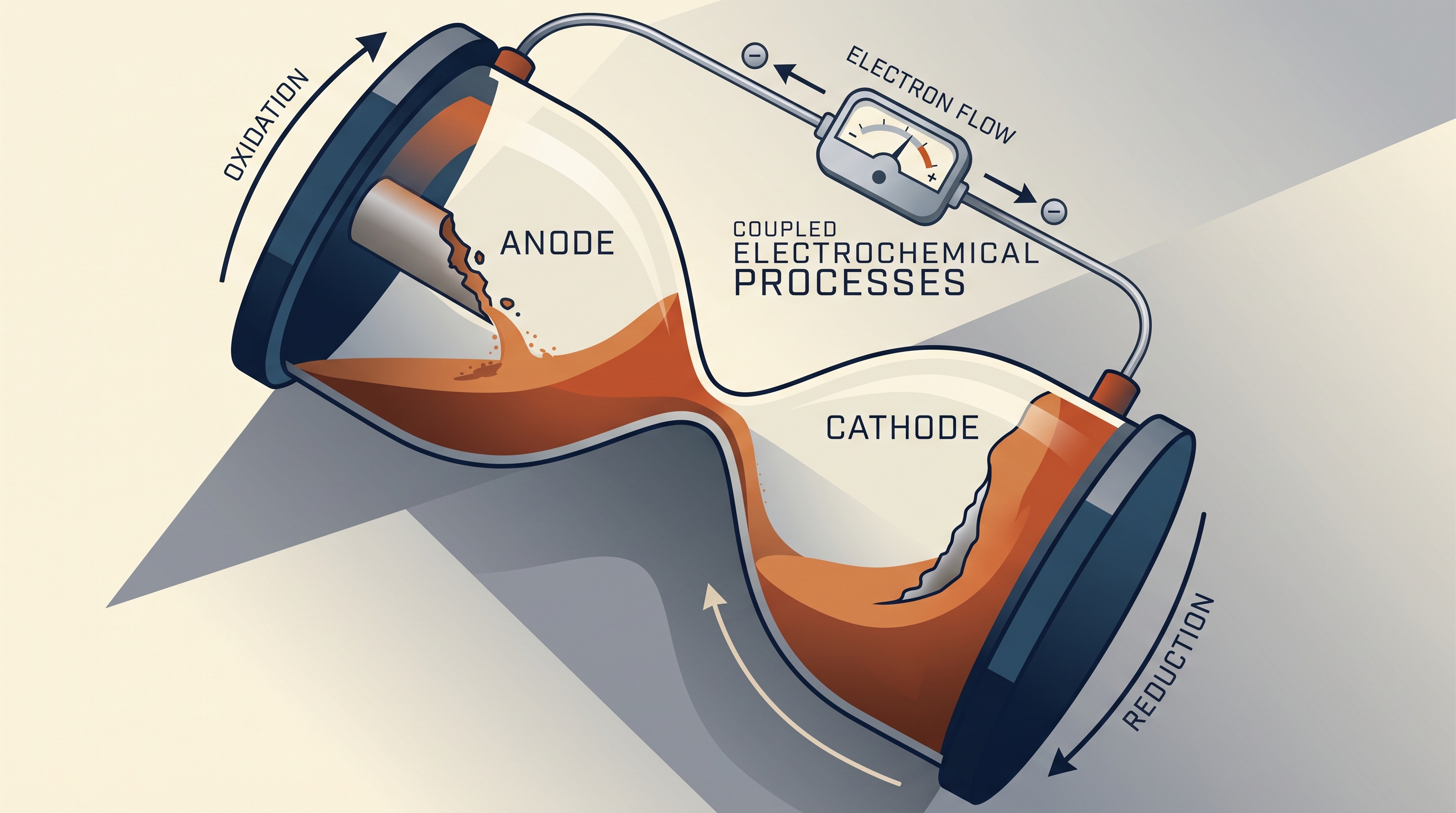
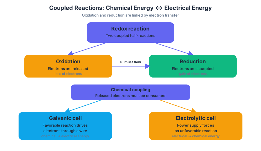
9.9 Cell Potential and Free Energy · 9.10 Cell Potential Under Nonstandard Conditions
Key concepts: Standard cell potential (E°cell) · Cell potential under nonstandard conditions · Relationship between cell potential and Gibbs free energy · Relationship among E°, ΔG°, K, and temperature · Standard reduction potentials · Oxidation and reduction half-reactions · Reaction quotient (Q) · Nernst equation · Spontaneity and equilibrium in electrochemical cells · Effects of deviations from standard conditions
A cell voltage is more than a meter reading: it reveals whether a redox reaction is thermodynamically favored and how strongly the reaction is being driven.
9.9 Cell Potential and Free Energy · 9.10 Cell Potential Under Nonstandard Conditions
A cell voltage is more than a meter reading: it reveals whether a redox reaction is thermodynamically favored and how strongly the reaction is being driven. The central question is, how do half-reactions, free energy, equilibrium, and concentration combine to determine the voltage of an electrochemical cell?
From half-reactions to standard cell potential
A standard reduction potential, written $E^\circ_{\text{red}}$, measures the tendency of a reduction half-reaction to gain electrons under standard conditions. Standard reduction potentials are listed as reductions, even when a particular cell uses one of them in reverse as an oxidation.
9.9.A.2: Calculate the standard cell potential by identifying the oxidation and reduction half-reactions and combining their standard reduction potentials.
For a galvanic cell, reduction occurs at the cathode and oxidation occurs at the anode. Because tabulated values are reduction potentials, use:
$$ E^\circ_{\text{cell}}
E^\circ_{\text{red,cathode}}
E^\circ_{\text{red,anode}} $$
Do not multiply a potential by a coefficient when balancing electrons. Potential is an intensive quantity: reversing a half-reaction changes the sign of its potential, but multiplying the half-reaction does not change the potential.
Worked example: finding $E^\circ_{\text{cell}}$
Consider the following balanced half-reactions:
$$ 2\text{MnO}_2(s)+\text{H}_2\text{O}(l)+2e^- \rightarrow \text{Mn}_2\text{O}_3(s)+2\text{OH}^-(aq) $$
$$ \text{Zn}(s)+2\text{OH}^-(aq) \rightarrow \text{ZnO}(s)+\text{H}_2\text{O}(l)+2e^- $$
The manganese reaction is reduction and has $E^\circ_{\text{red}}=0.15\ \text{V}$. The zinc reaction is oxidation, but its listed reduction potential is $-1.28\ \text{V}$. Therefore:
$$ E^\circ_{\text{cell}}
0.15\ \text{V}-(-1.28\ \text{V})
1.43\ \text{V} $$
The positive value indicates that the overall reaction is thermodynamically favored under standard conditions. The balanced overall reaction is:
$$ 2\text{MnO}_2(s)+\text{Zn}(s) \rightarrow \text{Mn}_2\text{O}_3(s)+\text{ZnO}(s) $$
Here, $n=2$ mol $e^-$ are transferred per mole of reaction. That electron count comes from the balanced redox equation, not from whichever half-reaction happens to be written first.
Cell potential and Gibbs free energy
Standard Gibbs free energy change, $\Delta G^\circ$, describes the thermodynamic driving force for a reaction under standard conditions. For an electrochemical reaction:
$$ \Delta G^\circ=-nFE^\circ_{\text{cell}} $$
where $n$ is the number of moles of electrons transferred per mole of reaction and $F$ is Faraday’s constant:
$$ F=96{,}485\ \text{C mol}^{-1}e^- $$
For the manganese–zinc cell:
$$ \Delta G^\circ
-(2)(96{,}485\ \text{C mol}^{-1}e^-)(1.43\ \text{J C}^{-1}) $$
$$ \Delta G^\circ
-2.76\times10^5\ \text{J mol}^{-1}_{\text{rxn}}
-276\ \text{kJ mol}^{-1}_{\text{rxn}} $$
The signs form a required three-way connection:
| Standard cell potential | $\Delta G^\circ$ | Thermodynamic interpretation |
|---|---|---|
| $E^\circ_{\text{cell}}>0$ | $\Delta G^\circ<0$ | Forward reaction is favored |
| $E^\circ_{\text{cell}}=0$ | $\Delta G^\circ=0$ | System is at equilibrium |
| $E^\circ_{\text{cell}}<0$ | $\Delta G^\circ>0$ | Forward reaction is unfavored |
A positive $E^\circ_{\text{cell}}$ predicts a thermodynamically favored spontaneous reaction under standard conditions. “Spontaneous” does not mean “fast”: kinetics determines how rapidly a reaction occurs, while $\Delta G^\circ$ determines its thermodynamic favorability.
Connecting $E^\circ$, $\Delta G^\circ$, and $K$
At equilibrium, the reaction has no remaining thermodynamic driving force, so $\Delta G=0$. Combining
with
$$ \Delta G^\circ=-RT\ln K $$
gives:
$$ \ln K=\frac{nFE^\circ_{\text{cell}}}{RT} $$
Here, $R$ is the gas constant and $T$ is absolute temperature in kelvins.
Thus, at a fixed temperature, a positive $E^\circ_{\text{cell}}$ corresponds to $\ln K>0$, so $K>1$. Products are favored at equilibrium under standard conditions. A negative $E^\circ_{\text{cell}}$ corresponds generally to $K<1$, meaning reactants are favored.
Nonstandard conditions: why the voltage changes
Standard conditions are a reference state, not the only state in which a cell operates. Under nonstandard conditions, the cell potential depends on the concentrations or other activities of the active species through the reaction quotient, $Q$.
For a general reaction
$$ aA+bB\rightarrow cC+dD $$
the reaction quotient is
$$ Q=\frac{a_C^c a_D^d}{a_A^a a_B^b} $$
where $a_i$ represents the activity of each active species. Pure solids and pure liquids are omitted because their activities are treated as constant.
The Nernst equation expresses the change:
$$ E_{\text{cell}}
E^\circ_{\text{cell}}
\left(\frac{RT}{nF}\right)\ln Q $$
In this equation, $n$ is the number of electrons transferred, $R$ is the gas constant, $T$ is temperature in kelvins, and $F$ is Faraday’s constant.
The most useful reasoning is qualitative:
- If $Q=1$, then $\ln Q=0$, so $E_{\text{cell}}=E^\circ_{\text{cell}}$.
- If $Q<1$, then $\ln Q<0$, so subtracting it increases $E_{\text{cell}}$.
- If $Q>1$, then $\ln Q>0$, so $E_{\text{cell}}$ decreases.
- As $Q$ approaches $K$, the system approaches equilibrium and the driving force decreases.
- At equilibrium, $Q=K$ and $E_{\text{cell}}=0$.
For the manganese–zinc reaction, the solids are omitted:
$$ Q=\frac{a_{\text{Mn}_2\text{O}3}}{a{\text{MnO}_2}^2} $$
If the solid activities remain effectively constant, $Q$ is approximately constant as well. In a cell reaction containing dissolved ions or gases, however, changing an active species can shift $Q$ and therefore change the measured voltage.
A concentration thought experiment
Suppose a reaction consumes aqueous reactants and produces aqueous products. Adding reactant decreases $Q$. The Nernst equation then predicts an increase in $E_{\text{cell}}$, because the system is farther from equilibrium in the forward direction and has a larger driving force.
Adding product increases $Q$, which lowers $E_{\text{cell}}$. The reaction still may proceed forward if $Q<K$, but it proceeds with less electrical driving force than it had under standard conditions.
Misconception check
Misconception: “A positive cell potential means the reaction is fast.”
Correction: $E_{\text{cell}}>0$ means the reaction is thermodynamically favored in the written direction. It says nothing by itself about activation energy or reaction rate.
Misconception: “Increasing every concentration always increases the voltage.”
Correction: only the effect on $Q$ matters. Increasing a reactant concentration usually decreases $Q$ and raises $E_{\text{cell}}$; increasing a product concentration usually raises $Q$ and lowers $E_{\text{cell}}$. Stoichiometric exponents also matter.
Misconception: “The Nernst equation is mainly a substitution exercise.”
Correction: 9.10.A.4 emphasizes qualitative reasoning. Before calculating, determine whether the change makes $Q$ larger or smaller and whether the cell moves toward or away from equilibrium.
AP skill connection and retrieval check
This topic most directly develops Science Practice 5: Mathematical Routines when calculating $E^\circ_{\text{cell}}$, $\Delta G^\circ$, $\ln K$, or $E_{\text{cell}}$. It also develops Science Practice 4: Model Analysis when interpreting half-reactions, potential diagrams, and the Nernst equation, and Science Practice 6: Argumentation when justifying favorability from the signs of $E^\circ_{\text{cell}}$ and $\Delta G^\circ$.
Retrieval check: A cell has $E^\circ_{\text{cell}}=0.80\ \text{V}$. If the reaction quotient increases from $Q=1$ to $Q>1$, does $E_{\text{cell}}$ increase or decrease, and why?
Answer: It decreases because $\ln Q$ becomes positive, so the Nernst correction is subtracted from $E^\circ_{\text{cell}}$. The reaction is moving toward equilibrium, so its driving force becomes smaller.
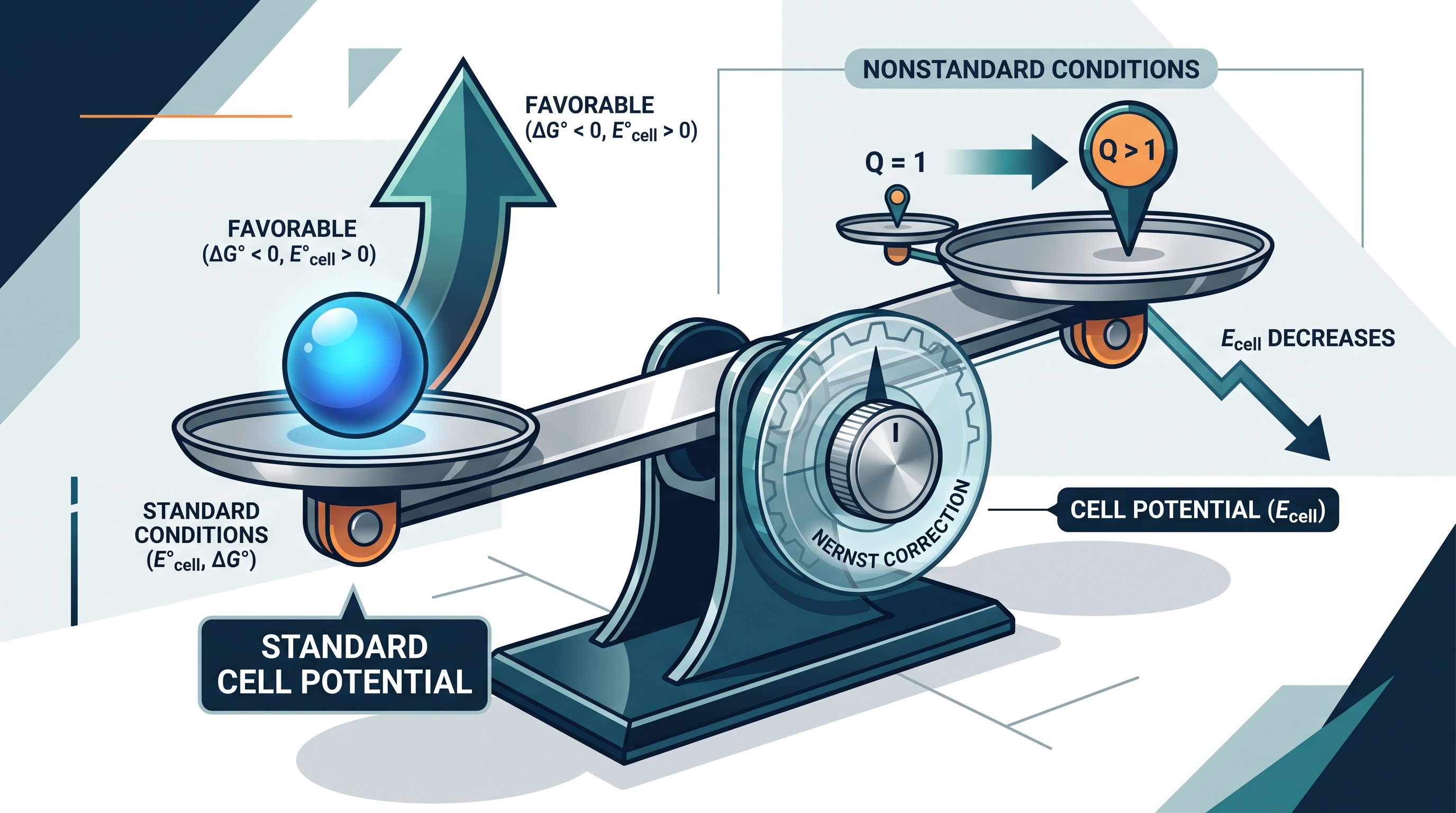
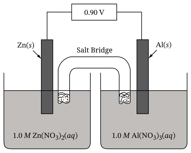
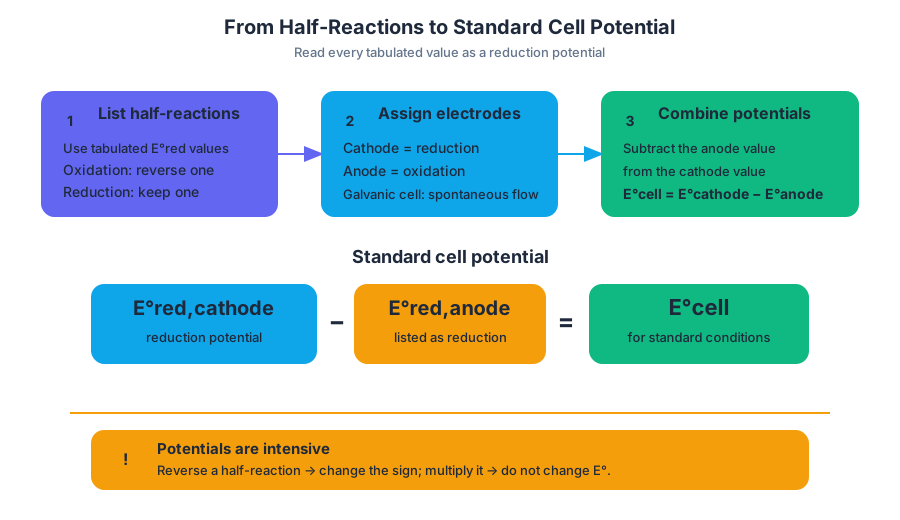
9.11 Electrolysis and Faraday’s Law
Key concepts: Electrolysis · Faraday’s law · Nonspontaneous redox reactions · Thermodynamic spontaneity · External power sources · Stoichiometric calculations · Moles of electrons and electric charge · Current, charge, and time · Standard reduction potentials · Cell potential under nonstandard conditions
Electrolysis uses an external power source to force a redox reaction that would not proceed spontaneously. In an electrolytic cell, electrical energy becomes chemical change: metal ions may be reduced and deposited onto an electrode, or a solid electrode may be oxidized and removed.
9.11 Electrolysis and Faraday’s Law
Electrolysis uses an external power source to force a redox reaction that would not proceed spontaneously. In an electrolytic cell, electrical energy becomes chemical change: metal ions may be reduced and deposited onto an electrode, or a solid electrode may be oxidized and removed.
9.11.A — Calculate the amount of charge flow based on changes in the amounts of reactants and products in an electrochemical cell.
The central bridge is Faraday’s law: the amount of material changed at an electrode is proportional to the amount of charge transferred. The microscopic count of electrons connects to the macroscopic quantities measured in the laboratory—mass, current, and elapsed time.
Spontaneity and the need for an external power source
A galvanic cell produces electrical energy from a spontaneous reaction. For the reaction as written,
$$\Delta G^\circ=-nFE^\circ_{\text{cell}}$$
where $n$ is the number of moles of electrons transferred and $F$ is Faraday’s constant, approximately $96{,}485\ \text{C mol}^{-1}e^-$. Thus, a positive $E^\circ_{\text{cell}}$ corresponds to $\Delta G^\circ<0$ and a spontaneous reaction.
Electrolysis reverses that energy flow. The desired reaction has $\Delta G>0$ and, under the relevant conditions, a negative cell potential. An external power source supplies the energy needed to push electrons in the nonspontaneous direction. Under actual, nonstandard conditions, the cell potential for those conditions—not automatically the standard value—determines whether the forced reaction is nonspontaneous.
Misconception check — “A positive cell potential requires a battery.” A positive $E_{\text{cell}}$ indicates a spontaneous cell reaction. It is a negative cell potential for the reaction as written that signals the need for an external power source in electrolysis.
Faraday’s law as an electron-counting pipeline
For any electrolytic calculation, begin with the balanced electrode half-reaction. The coefficient of $e^-$ gives the required electron-to-substance ratio. Then use dimensional analysis:
$$ \text{mass} \rightarrow \text{moles of substance} \rightarrow \text{moles of }e^- \rightarrow \text{coulombs} \rightarrow \text{seconds} $$
The essential knowledge is 9.11.A.1 — Faraday’s laws can be used to determine the stoichiometry of the redox reaction occurring in an electrochemical cell with respect to the number of electrons transferred, mass of material deposited on or removed from an electrode, current, time elapsed, and charge of ionic species.
The quantitative relationships are
$$ q=n_{e^-}F $$
and
$$ I=\frac{q}{t} $$
where $q$ is charge in coulombs, $n_{e^-}$ is moles of electrons, $I$ is current in amperes, and $t$ is time in seconds. Since $1\ \text{A}=1\ \text{C s}^{-1}$,
$$ t=\frac{q}{I}. $$
Worked example: plating rhodium
Suppose $2.8\ \text{g}$ of rhodium is plated from $\text{Rh}^{3+}(aq)$ at a current of $2.0\ \text{C s}^{-1}$. The reduction half-reaction is
$$ \text{Rh}^{3+}(aq)+3e^-\rightarrow\text{Rh}(s). $$
Therefore, $3$ moles of electrons are required for every $1$ mole of rhodium deposited.
First convert the deposited mass to moles of rhodium and then to moles of electrons:
$$ 2.8\ \text{g Rh} \left(\frac{1\ \text{mol Rh}}{102.91\ \text{g Rh}}\right) \left(\frac{3\ \text{mol }e^-}{1\ \text{mol Rh}}\right) =0.082\ \text{mol }e^-. $$
Convert electrons to charge and charge to time:
$$ 0.082\ \text{mol }e^- \left(\frac{96{,}485\ \text{C}}{1\ \text{mol }e^-}\right) \left(\frac{1\ \text{s}}{2.0\ \text{C}}\right) \approx 3.9\times10^3\ \text{s}. $$
The required charge is approximately
$$ q=(0.082)(96{,}485)\approx 7{,}868.68\ \text{C}, $$
and the required time is approximately
$$ t\approx3{,}900\ \text{s}. $$
The answer has two significant figures because both $2.8\ \text{g}$ and $2.0\ \text{C s}^{-1}$ have two significant figures.
Common error: using a $1:1$ ratio between moles of Rh and moles of electrons. The ionic charge controls the ratio: reducing $\text{Rh}^{3+}$ requires $3$ electrons per rhodium atom.
The same method for material removed
Faraday’s law applies equally when an electrode dissolves. For a metal with ionic charge $z+$, oxidation is represented by
$$ \text{M}(s)\rightarrow\text{M}^{z+}(aq)+ze^-. $$
If $m$ grams of $\text{M}(s)$ are removed, calculate
$$ m \left(\frac{1\ \text{mol M}}{\text{molar mass of M}}\right) \left(\frac{z\ \text{mol }e^-}{1\ \text{mol M}}\right) \left(\frac{96{,}485\ \text{C}}{1\ \text{mol }e^-}\right). $$
For example, removing $1.00\ \text{g}$ of a metal that oxidizes as
$$ \text{M}(s)\rightarrow\text{M}^{2+}(aq)+2e^- $$
requires twice as many moles of electrons per mole of metal as a $1+$ metal. The mass–moles–electrons–charge chain is unchanged; only the half-reaction and molar mass change.
Exam reasoning and retrieval check
A complete response should show the balanced redox half-reaction or net ionic equation, identify the electron ratio, carry units through each conversion, and report an answer with appropriate significant figures. This develops Science Practice 5: Mathematical Routines, while the half-reaction and electron-flow model engage Science Practice 1: Models and Representations and Science Practice 4: Model Analysis.
Retrieval check: An electrode loses $0.500\ \text{g}$ of a metal through $\text{M}(s)\rightarrow\text{M}^{3+}(aq)+3e^-$. Before calculating, identify the controlling ratio: how many moles of electrons are released per mole of metal? If the answer is not $3$, the half-reaction has not yet been used correctly.
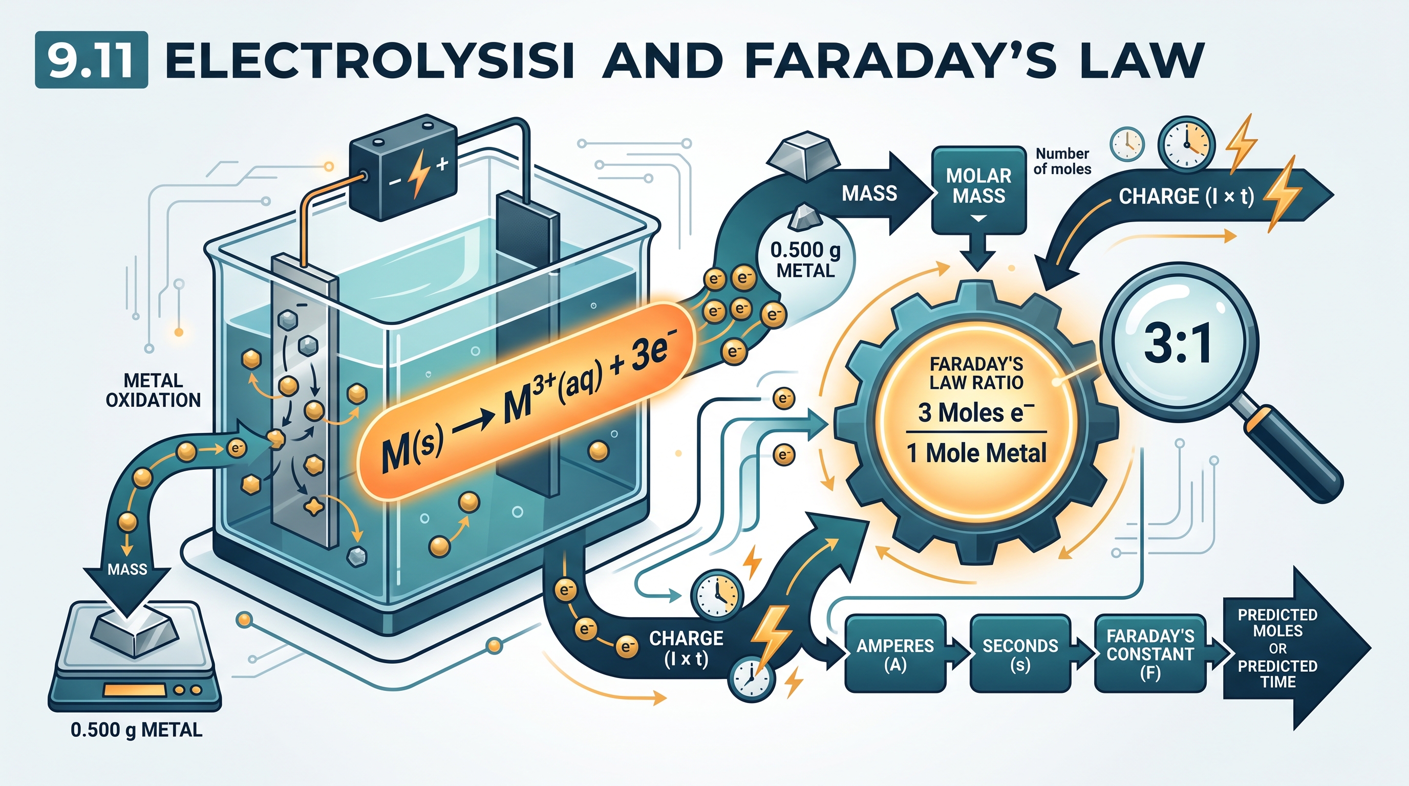
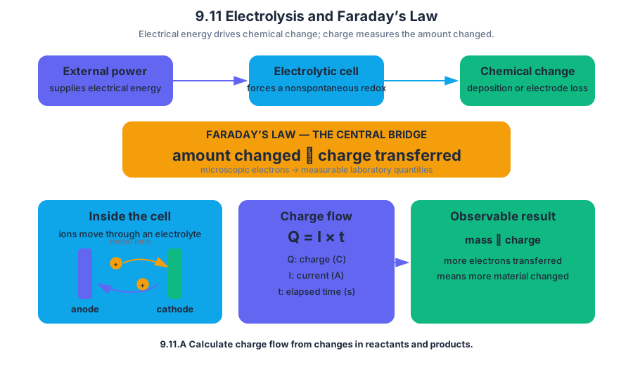
AP Practice 1
Key concepts: AP principles of clarity and transparency through publicly available course frameworks and sample exam questions · AP opposition to indoctrination and emphasis on analyzing multiple perspectives · Evidence-based discussion in which students evaluate arguments rather than one another · Respect for diversity in students’ backgrounds, experiences, and viewpoints · AP Chemistry course organization into units on properties of substances and mixtures, chemical reactions, kinetics, thermochemistry, equilibrium, acids and bases, and thermodynamics and electrochemistry · Laboratory investigation practices, including experimental design, prediction, data collection and analysis, mathematical routines, explanation, and communication · Use of formative assessment, such as Progress Checks, to identify and address student misunderstandings · Mass spectrometry as a tool for analyzing isotopic abundance and identifying elements in mixtures
A mass spectrum can turn an invisible isotope mixture into measurable evidence: peak position identifies isotope mass, while peak intensity reveals relative abundance. That same reasoning appears in forensic science, where isotope patterns can help distinguish substances, identify an element in a mixture, or…
AP Practice 1
A mass spectrum can turn an invisible isotope mixture into measurable evidence: peak position identifies isotope mass, while peak intensity reveals relative abundance. That same reasoning appears in forensic science, where isotope patterns can help distinguish substances, identify an element in a mixture, or calculate an element’s average atomic mass.
The AP Program makes its course frameworks, unit descriptions, science practices, and sample exam questions publicly available. These materials make expectations transparent: students can see not only what chemistry is assessed, but also whether they must represent data, analyze a model, perform a mathematical routine, design an investigation, or justify a claim with evidence.
The task type: data-based multiple choice
This practice uses an original multiple-choice question built around a scientific representation. On the current AP Chemistry Exam, multiple-choice questions may require a student to move among a spectrum, a numerical calculation, a particulate interpretation, and a chemical conclusion. The strongest approach is not to guess from a familiar pattern; it is to identify what each datum means and connect it to the claim being tested.
Science Practice 3: Representing Data and Phenomena means translating observations into useful representations and interpreting what those representations show.
The question also uses Science Practice 5: Mathematical Routines, because isotope abundance must be converted into a weighted average. It touches Science Practice 6: Argumentation when the calculated result is used as evidence for identifying an element.
Original practice question
A forensic laboratory analyzes a pure element recovered from a small metal fragment. Its mass spectrum contains two major peaks:
| Isotope | Isotopic mass | Relative abundance |
|---|---|---|
| $X$-63 | $63.0\ \mathrm{u}$ | $69.0%$ |
| $X$-65 | $65.0\ \mathrm{u}$ | $31.0%$ |
Which statement is best supported by the spectrum?
A. The sample is a mixture of two elements, because it produces two peaks.
B. The average atomic mass of the element is $64.0\ \mathrm{u}$.
C. The average atomic mass of the element is approximately $63.6\ \mathrm{u}$, consistent with an element whose naturally occurring isotopes have masses near $63\ \mathrm{u}$ and $65\ \mathrm{u}$.
D. The $X$-65 isotope contains two more protons than the $X$-63 isotope.
Worked reasoning
The two peaks have different masses but represent isotopes of the same element. Isotopes have the same number of protons and different numbers of neutrons, so the two peaks do not by themselves prove that two elements are present.
Convert each percentage to a decimal fraction, multiply each isotope’s mass by its abundance, and add:
$$ \text{average atomic mass}
(63.0\ \mathrm{u})(0.690)+(65.0\ \mathrm{u})(0.310) $$
$$ \text{average atomic mass}
43.47\ \mathrm{u}+20.15\ \mathrm{u}
63.62\ \mathrm{u} $$
The result is approximately $63.6\ \mathrm{u}$, so C is correct. The average lies closer to $63.0\ \mathrm{u}$ because the $X$-63 isotope is more abundant.
Examiner-rewarded reasoning: interpret peak positions as isotope masses, interpret intensities as relative abundances, use a weighted average rather than an ordinary mean, and connect the numerical result to an evidence-based identification.
Why the other choices fail
A confuses isotopes with elements. A mass spectrum showing two isotope peaks can be evidence for one element with two isotopes. A mixture of elements would be supported only if the pattern contained isotope masses belonging to different elements.
B uses the unweighted average, $(63.0+65.0)/2$, which assumes equal abundance. The abundances are not equal, so the average must be closer to $63.0\ \mathrm{u}$.
D confuses atomic number with mass number. The isotope labels differ by two mass units, meaning the nuclei differ by two neutrons, not two protons. Changing the number of protons changes the element.
Evidence, perspectives, and respectful argument
AP points are awarded for chemically correct evidence and reasoning, not for agreement with a particular political, cultural, or personal viewpoint. When a chemistry claim has competing interpretations—for example, whether a spectrum represents a pure element or a mixture—students should compare the assumptions, data, and explanatory power of each interpretation.
A productive discussion evaluates arguments rather than classmates. Students may bring different backgrounds, experiences, and viewpoints to questions involving forensic science, environmental chemistry, medicine, or technology. Those differences deserve respect; personal attacks do not belong in evidence-based scientific discussion. Primary data and reliable sources should decide the chemical claim.
Laboratory practice behind the question
The same reasoning cycle extends beyond a multiple-choice item:
$$ \text{question} \rightarrow \text{method} \rightarrow \text{prediction} \rightarrow \text{data collection} \rightarrow \text{analysis} \rightarrow \text{explanation} \rightarrow \text{communication} $$
In an AP Chemistry laboratory investigation, students may design an experiment, predict an outcome, collect measurements, apply mathematical routines, analyze uncertainty or patterns, develop an explanation, and communicate a conclusion supported by evidence. Colleges may ask students to present laboratory notebooks, reports, or other materials before awarding credit for laboratory work, so clear documentation matters beyond the exam.
Where this task fits in the course
Mass spectra belong especially to Unit 1: Atomic Structure and Properties, while the interpretation habits used here spiral through the course. The AP Chemistry units and their multiple-choice weightings are:
| Unit | Course focus | Exam weighting |
|---|---|---|
| Unit 1 | Atomic Structure and Properties | $7$–$9%$ |
| Unit 2 | Compound Structure and Properties | $7$–$9%$ |
| Unit 3 | Properties of Substances and Mixtures | $18$–$22%$ |
| Unit 4 | Chemical Reactions | $7$–$9%$ |
| Unit 5 | Kinetics | $7$–$9%$ |
| Unit 6 | Thermochemistry | $7$–$9%$ |
| Unit 7 | Equilibrium | $7$–$9%$ |
| Unit 8 | Acids and Bases | $11$–$15%$ |
| Unit 9 | Thermodynamics and Electrochemistry | $7$–$9%$ |
A schedule of five $45$-minute class periods per week is a planning suggestion, not a fixed rule. Block schedules, school calendars, student needs, and the time required for laboratory investigations may justify different pacing.
Progress Check and error review
Use a short Progress Check diagnostically rather than treating its score as the end of learning. For this question, classify an error precisely:
- Representation error: peak intensity was not recognized as abundance.
- Mathematical-routine error: percentages were not converted to decimal fractions.
- Conceptual error: isotopes were confused with different elements.
- Argumentation error: the conclusion was stated without connecting it to the spectrum.
Reteach only the diagnosed misconception, then complete a follow-up check using a new spectrum with different masses and abundances. A student is ready to move on when the calculation, interpretation, and evidence-based conclusion all agree—not merely when the final letter choice is correct.
Timing guidance: spend about $2$ minutes identifying what the peaks encode, $1$ minute calculating, and $1$ minute checking whether the result is closer to the more abundant isotope.

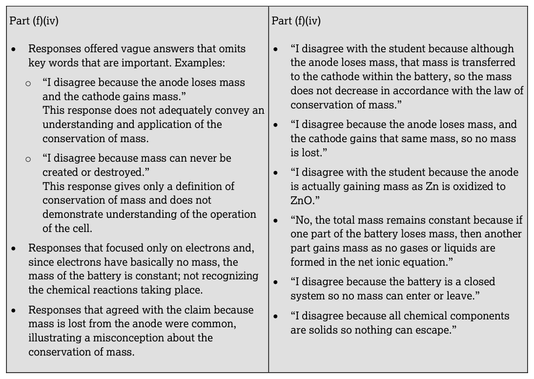
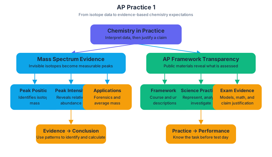
AP Practice 2
Key concepts: Prerequisites for AP Chemistry · Laboratory instruction and hands-on investigations · Mole concept and dimensional analysis · Graphing experimental data with correct scales and units · Solubility product constants (Ksp) and ionic factors · Electrolysis · Stoichiometry involving changing or limiting/excess reactants · Particulate representations of matter · Chemical polarity and polarizability · Acid-base titration curves
A single laboratory investigation can force several kinds of chemical reasoning at once: converting masses with the mole concept, plotting data with defensible scales, interpreting particulate models, predicting precipitation with $K_{sp}$, and explaining electrolysis through electron transfer.
AP Practice 2
A single laboratory investigation can force several kinds of chemical reasoning at once: converting masses with the mole concept, plotting data with defensible scales, interpreting particulate models, predicting precipitation with $K_{sp}$, and explaining electrolysis through electron transfer. The practice task below is an original, unofficial short free-response problem designed around that integration.
Prerequisite readiness: Successful work assumes an introductory high school chemistry course and Algebra II, or equivalent preparation. You should be comfortable with balanced equations, proportional reasoning, scientific notation, logarithms, and unit conversions.
The laboratory context
A student investigates a solution containing an unknown weak acid, then studies the solubility of lead(II) iodide and finally deposits copper by electrolysis. The laboratory sequence reflects the expected emphasis on experimentation: at least $25%$ of instructional time should involve hands-on laboratory work, with teachers conducting at least $16$ hands-on investigations.
The student records titration data as pH versus volume of base added. A scientifically useful graph must place the independent variable, volume of base, on the horizontal axis and pH on the vertical axis. Both axes require numerical scales, units where applicable, and enough range to reveal the steep region near the equivalence point.
A good graph is not merely a picture of the data. It is a representation of a chemical phenomenon, satisfying Skill 3.A: Represent chemical phenomena using appropriate graphing techniques, including correct scale and units. A smooth-looking curve cannot repair missing units, uneven scale intervals, or incorrectly assigned axes.
Original short free-response task
A student titrates $25.00\ \mathrm{mL}$ of a weak monoprotic acid with $0.1000\ \mathrm{M}$ sodium hydroxide. The pH-versus-volume data show the sharpest increase between $23.8\ \mathrm{mL}$ and $24.2\ \mathrm{mL}$ of base added.
(a) Identify the approximate equivalence-point volume and describe one graphing feature that should appear near that volume.
(b) At the equivalence point, the student has added $24.0\ \mathrm{mL}$ of $0.1000\ \mathrm{M}$ $NaOH$. Calculate the initial moles of weak acid.
(c) A separate sample contains $Pb^{2+}$ and is tested by adding one drop of $0.100\ \mathrm{M}$ $KI$. Write the net ionic equation for the precipitate formation and explain why ion charge is important when comparing solubility patterns.
(d) During electrolysis of aqueous $CuSO_4$, copper forms at the cathode. Identify whether the cathode process is oxidation or reduction and justify the answer using electrons.
Worked solution and scoring logic
(a) Equivalence point. The approximate equivalence volume is $24.0\ \mathrm{mL}$ because it lies in the center of the steepest pH change. The graph should show a rapid rise in pH near this volume, not necessarily a pH of $7.00$.
This earns the reasoning associated with identifying a chemical feature from a graph and supports Skill 3.A: Represent chemical phenomena using appropriate graphing techniques, including correct scale and units. A strong response connects the equivalence point to the sharp change in pH rather than simply choosing the largest recorded pH.
(b) Mole calculation.
$$ n(NaOH)=M V $$
$$ n(NaOH)=\left(0.1000\ \mathrm{mol,L^{-1}}\right) \left(0.0240\ \mathrm{L}\right) =2.40\times10^{-3}\ \mathrm{mol} $$
The acid is monoprotic, so the neutralization ratio is $1:1$:
$$ HA+OH^-\rightarrow A^-+H_2O $$
$$ n(HA)=n(OH^-)=2.40\times10^{-3}\ \mathrm{mol} $$
The calculation demonstrates Skill 5.F: Calculate, estimate, or predict an unknown quantity from known quantities by selecting and following a logical computational pathway and attending to precision, including dimensional analysis and significant figures. The volume must be converted from milliliters to liters before using molarity.
(c) Lead(II) iodide precipitation.
The net ionic equation is
Pb^{2+}(aq)+2I^-(aq)\rightleftharpoons PbI_2(s)
The ion charge matters because the solubility equilibrium contains the ion concentrations raised to stoichiometric powers:
$$ K_{sp}=[Pb^{2+}][I^-]^2 $$
A small amount of $0.100\ \mathrm{M}$ $KI$ can supply enough $I^-$ to make the ionic product exceed $K_{sp}$, causing precipitation. In comparing compounds, examine ion charge, ionic radius, and whether the ions are polyatomic or monoatomic; these structural factors influence lattice attractions and hydration, so solubility cannot be predicted from charge alone.
This response uses Skill 6.C: Support a claim with evidence from representations or models at the particulate level, such as the structure of atoms and/or molecules, and Skill 6.E: Provide reasoning to justify a claim using connections between particulate and macroscopic scales or levels. The particulate event—ions combining into a solid lattice—explains the visible cloudiness or precipitate.
(d) Electrolysis. Copper forms at the cathode by reduction:
$$ Cu^{2+}(aq)+2e^-\rightarrow Cu(s) $$
The cathode is defined by reduction, regardless of whether the cell is galvanic or electrolytic. The external power source forces this nonspontaneous process to occur. A response that says “cathode is negative, therefore reduction” is incomplete: the electron gain is the chemical justification.
Common traps
Misconception: equivalence always means neutral pH.
A strong acid–strong base titration has an equivalence point near pH $7$, but a weak acid–strong base titration has a basic equivalence solution because $A^-$ reacts with water.
Misconception: more $KI$ always means a proportionally larger precipitate.
Precipitation depends on the ionic product relative to $K_{sp}$. Once precipitation begins, dissolved-ion concentrations shift according to equilibrium; the process is not simply unrestricted mixing.
Misconception: oxidation occurs at the anode and reduction at the cathode only in batteries.
The locations are universal: oxidation at the anode, reduction at the cathode. What changes between galvanic and electrolytic cells is whether the reaction is spontaneous and how electrical energy is supplied.
Representation checkpoint
Draw three particulate-level snapshots for the lead(II) iodide test: before adding $KI$, immediately after ions mix, and after $PbI_2(s)$ forms. Then label which particles remain dissolved. This practices Skill 3.B: Represent chemical substances or phenomena with appropriate diagrams or models, while connecting symbolic equations to observable evidence.
Timing and error review
Allow approximately $9$ minutes for this short-response task: about $2$ minutes to read and plan, $5$ minutes to calculate and explain, and $2$ minutes to check units, equations, and labels. For each missed point, classify the error as concept, representation, mathematical routine, or argumentation; then rewrite the answer using a chemical equation, a labeled model, or a unit-carrying calculation.
Retrieval check: If the volume of $NaOH$ at equivalence doubled while its molarity stayed constant, what would happen to the calculated initial moles of $HA$? Explain using $n=MV$ and the $1:1$ reaction ratio.
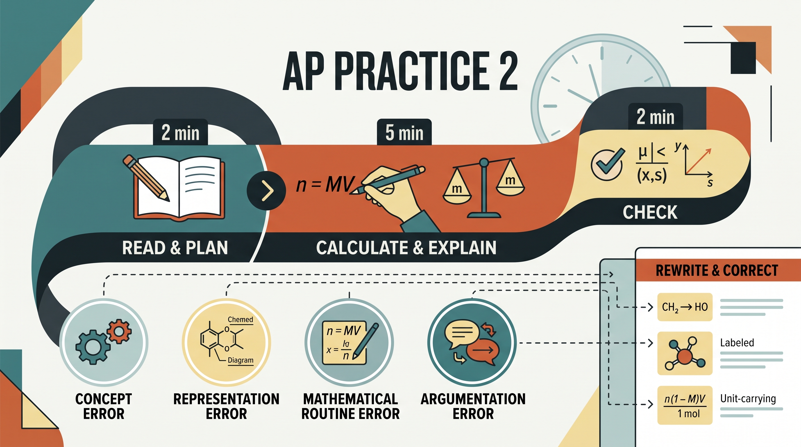
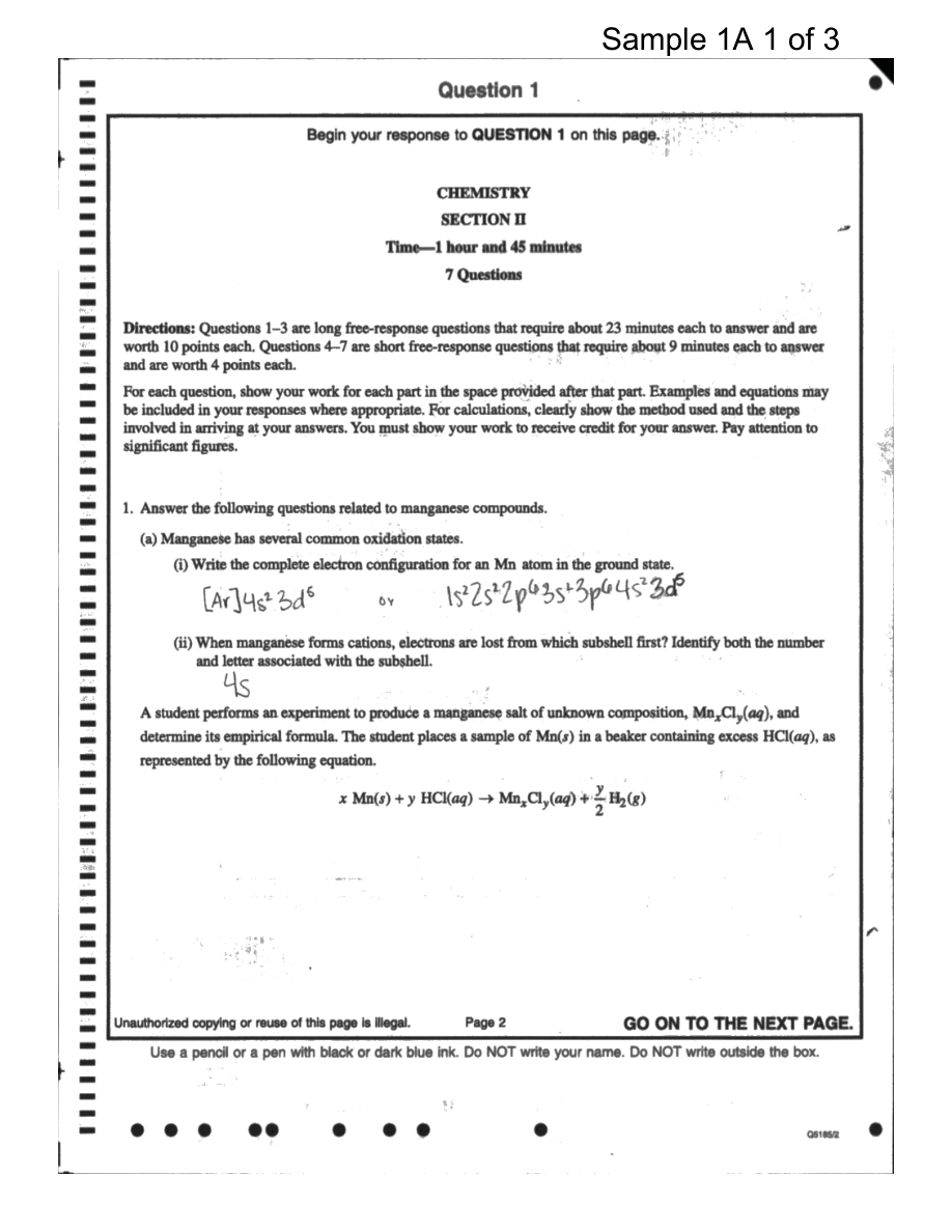
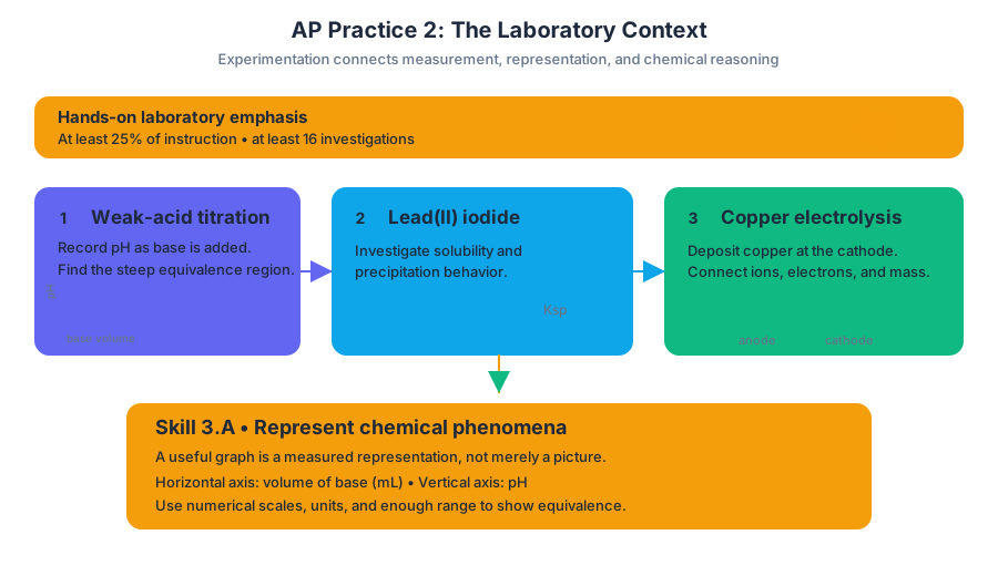
AP Practice 3
A strong chemistry argument does more than announce an answer: it connects a claim to chemical evidence and explains why the evidence supports that claim.
AP Practice 3
A strong chemistry argument does more than announce an answer: it connects a claim to chemical evidence and explains why the evidence supports that claim. This original short free-response question (FRQ) practices that exam task type through Science Practice 6: Argumentation, while also requiring Science Practice 4: Model Analysis and Science Practice 5: Mathematical Routines.
Task type: Original, unofficial short free-response question
Suggested time: $10$–$12$ minutes
Primary science practice: 6. Argumentation
Supporting science practices: 4. Model Analysis and 5. Mathematical Routines
The investigation: Which antacid neutralizes more acid?
Two powdered antacids, $A$ and $B$, are tested by adding separate samples to excess hydrochloric acid. The remaining acid is then measured by titration with $0.100\ \mathrm{M}$ sodium hydroxide. Because any acid left over requires sodium hydroxide to neutralize, a smaller volume of sodium hydroxide indicates that the antacid consumed more hydrochloric acid.
The balanced neutralization reaction is
$$ \mathrm{HCl}(aq)+\mathrm{NaOH}(aq)\rightarrow \mathrm{NaCl}(aq)+\mathrm{H_2O}(l) $$
Each antacid sample has a mass of $0.500\ \mathrm{g}$. The initial hydrochloric acid contains $0.0500\ \mathrm{mol}$ of $\mathrm{HCl}$. The titration results are shown below.
| Sample | Volume of $0.100\ \mathrm{M}$ $\mathrm{NaOH}$ used to titrate remaining $\mathrm{HCl}$ |
|---|---|
| Antacid $A$ | $18.0\ \mathrm{mL}$ |
| Antacid $B$ | $31.0\ \mathrm{mL}$ |
(a) Calculate the amount, in moles, of $\mathrm{HCl}$ remaining after reaction with antacid $A$.
(b) Determine which antacid consumed more $\mathrm{HCl}$ and support the conclusion with a quantitative argument using the data.
(c) A student claims that antacid $B$ must be more effective because it required a larger volume of $\mathrm{NaOH}$ during the titration. Evaluate the claim.
Worked reasoning
Part (a): Convert the titration measurement into chemical amount
The reaction ratio between $\mathrm{NaOH}$ and $\mathrm{HCl}$ is $1:1$. First convert the volume to liters:
$$ 18.0\ \mathrm{mL}=0.0180\ \mathrm{L} $$
Then use the molarity relationship:
$$ n=MV $$
$$ n_{\mathrm{NaOH}}=(0.100\ \mathrm{mol\ L^{-1}})(0.0180\ \mathrm{L}) =1.80\times10^{-3}\ \mathrm{mol} $$
Because the stoichiometric ratio is $1:1$,
$$ n_{\mathrm{HCl,\ remaining}}=1.80\times10^{-3}\ \mathrm{mol} $$
Point-worthy reasoning: The response must connect the measured sodium hydroxide volume to moles of sodium hydroxide, then use the balanced equation to identify the equal amount of remaining hydrochloric acid. A volume by itself is not yet a chemical amount.
Part (b): Build an evidence-based comparison
The initial amount of hydrochloric acid was
$$ n_{\mathrm{HCl,\ initial}}=0.0500\ \mathrm{mol} $$
For antacid $A$,
$$ n_{\mathrm{HCl,\ consumed}}
0.0500-0.00180
0.0482\ \mathrm{mol} $$
For antacid $B$, the amount of sodium hydroxide used is
$$ n_{\mathrm{NaOH}}
(0.100)(0.0310)
3.10\times10^{-3}\ \mathrm{mol} $$
Thus,
$$ n_{\mathrm{HCl,\ remaining}}=0.00310\ \mathrm{mol} $$
and
$$ n_{\mathrm{HCl,\ consumed}}
0.0500-0.00310
0.0469\ \mathrm{mol} $$
Antacid $A$ consumed more hydrochloric acid:
$$ 0.0482\ \mathrm{mol}>0.0469\ \mathrm{mol} $$
A complete argument is therefore: Antacid $A$ is more effective under these experimental conditions because less hydrochloric acid remained after treatment with $A$, so $A$ consumed $0.0482\ \mathrm{mol}$ of $\mathrm{HCl}$ compared with $0.0469\ \mathrm{mol}$ consumed by $B$.
Point-worthy reasoning: A high-scoring argument contains three linked parts: a clear claim, numerical evidence, and a chemical explanation connecting the evidence to the claim. Merely stating that $A$ is better does not establish the argument.
Part (c): Test the student’s interpretation
The student’s claim is incorrect. A larger volume of sodium hydroxide means that more hydrochloric acid remained to be titrated. Since antacid $B$ left $0.00310\ \mathrm{mol}$ of $\mathrm{HCl}$ while antacid $A$ left only $0.00180\ \mathrm{mol}$, $B$ neutralized less of the original acid.
Misconception check — “More titrant means more reacting power.”
In a back-titration, the titrant measures what is left over, not what the original substance consumed. A larger titrant volume can therefore indicate weaker performance by the tested material.
How the examiner sees the reasoning
| Response feature | What it demonstrates |
|---|---|
| Correctly uses $n=MV$ | 5. Mathematical Routines |
| Uses the $1:1$ reaction ratio | Chemical interpretation of a representation |
| Subtracts remaining acid from initial acid | Quantitative model analysis |
| Identifies antacid $A$ | Correct claim |
| Cites $0.0482\ \mathrm{mol}$ and $0.0469\ \mathrm{mol}$ | Relevant evidence |
| Explains why lower leftover acid means greater neutralization | 6. Argumentation |
A frequent weak response compares $18.0\ \mathrm{mL}$ and $31.0\ \mathrm{mL}$ without explaining what those volumes represent. The stronger response analyzes the experimental model: titration measures residual $\mathrm{HCl}$, and residual acid is inversely related to acid consumed when the initial amount is fixed.
Error-review routine
After completing the question, classify any error as one of four types: measurement conversion—forgetting $\mathrm{mL}$ to $\mathrm{L}$; stoichiometric interpretation—missing the $1:1$ ratio; comparison logic—confusing leftover acid with consumed acid; or argumentation—giving a claim without numerical evidence and chemical reasoning. Rewrite only the sentence containing the error, then recompute the result without looking at the solution.
Retrieval check: If the initial acid amount were identical but Sample $C$ required $10.0\ \mathrm{mL}$ of the same sodium hydroxide solution, would $C$ have consumed more or less hydrochloric acid than $A$? Explain using the meaning of the titration volume.

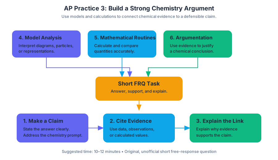
AP Practice 4
A strong long free-response answer does more than produce a number: it connects an observable result to a chemical model, supports a claim with evidence, and explains why the evidence supports the claim.
AP Practice 4
A strong long free-response answer does more than produce a number: it connects an observable result to a chemical model, supports a claim with evidence, and explains why the evidence supports the claim. This original practice task emphasizes experimental design, data representation, mathematical routines, model analysis, and scientific argumentation.
Task type: Long free-response question with experimental design
Recommended timing: $15$ minutes for a $10$-point question. Spend about $2$ minutes identifying variables and equations, $9$ minutes solving and explaining, and $4$ minutes checking units, significant figures, and cause-and-effect reasoning.
A student investigates the reaction between hydrogen peroxide and iodide ions in acidic solution:
$$ H_2O_2(aq)+2I^-(aq)+2H^+(aq)\rightarrow I_2(aq)+2H_2O(l) $$
The iodine produced reacts immediately with thiosulfate ions, allowing the student to measure the time required to produce a fixed amount of iodine. The initial-rate data are collected at constant temperature.
| Experiment | $[H_2O_2]$ ($\mathrm{mol,L^{-1}}$) | $[I^-]$ ($\mathrm{mol,L^{-1}}$) | $[H^+]$ ($\mathrm{mol,L^{-1}}$) | Initial rate ($\mathrm{mol,L^{-1},s^{-1}}$) |
|---|---|---|---|---|
| 1 | $0.100$ | $0.100$ | $0.0100$ | $2.00\times10^{-5}$ |
| 2 | $0.200$ | $0.100$ | $0.0100$ | $4.00\times10^{-5}$ |
| 3 | $0.100$ | $0.200$ | $0.0100$ | $8.00\times10^{-5}$ |
| 4 | $0.100$ | $0.100$ | $0.0200$ | $8.00\times10^{-5}$ |
Original practice prompt
(a) Write the rate law for the reaction using the experimental data. Show how the order with respect to each reactant is determined.
(b) Determine the value and units of the rate constant, $k$.
(c) The student proposes measuring reaction rate by recording the volume of oxygen gas produced rather than the iodine signal. Explain one advantage and one limitation of this method.
(d) Design an experiment to determine whether the reaction is first order or second order with respect to $H_2O_2$. Identify the independent variable, dependent variable, at least two controlled variables, and the evidence that would distinguish the two possible orders.
(e) Predict the initial rate when $[H_2O_2]=0.150\ \mathrm{mol,L^{-1}}$, $[I^-]=0.0500\ \mathrm{mol,L^{-1}}$, and $[H^+]=0.0100\ \mathrm{mol,L^{-1}}$.
Worked reasoning and scoring targets
(a) Determine the rate law
Assume
$$ \text{rate}=k[H_2O_2]^m[I^-]^n[H^+]^p $$
Compare Experiments $1$ and $2$: $[H_2O_2]$ doubles while the other concentrations remain constant. The rate also doubles, so $m=1$.
Compare Experiments $1$ and $3$: $[I^-]$ doubles, but the rate quadruples:
$$ \frac{8.00\times10^{-5}}{2.00\times10^{-5}}=4 $$
Therefore,
$$ 2^n=4 \qquad\Rightarrow\qquad n=2 $$
Compare Experiments $1$ and $4$: $[H^+]$ doubles, and the rate quadruples. Thus,
$$ 2^p=4 \qquad\Rightarrow\qquad p=2 $$
The rate law is therefore
$$ \boxed{\text{rate}=k[H_2O_2][I^-]^2[H^+]^2} $$
Credit target: The response must use controlled comparisons and connect each concentration change to the corresponding rate change. Merely stating the exponents earns less scientific reasoning than showing the ratio analysis.
(b) Calculate $k$
Using Experiment $1$:
$$ 2.00\times10^{-5} =k(0.100)(0.100)^2(0.0100)^2 $$
The concentration factor is
$$ (0.100)(0.100)^2(0.0100)^2 =1.00\times10^{-7} $$
Thus,
$$ k=\frac{2.00\times10^{-5}}{1.00\times10^{-7}} =2.00\times10^2 $$
The overall reaction order is
$$ 1+2+2=5 $$
Because
$$ [\text{rate}]=\mathrm{mol,L^{-1},s^{-1}} $$
the units of $k$ are
$$ \frac{\mathrm{mol,L^{-1},s^{-1}}} {(\mathrm{mol,L^{-1}})^5} =\boxed{\mathrm{L^4,mol^{-4},s^{-1}}} $$
Credit target: A complete answer includes the numerical value, the overall order used to determine units, and units consistent with the rate law. A frequent error is assigning $\mathrm{s^{-1}}$ automatically; that unit applies only to a first-order rate constant.
(c) Compare measurement methods
Measuring oxygen volume could provide a direct physical signal that increases as hydrogen peroxide decomposes, and gas volume can be recorded continuously with a pressure sensor or gas syringe. However, the proposed reaction equation produces iodine, not oxygen, so oxygen measurement would require a different reaction pathway or an additional decomposition reaction. Gas leakage, water vapor, and gas solubility could also introduce systematic error.
This response demonstrates Science Practice 1: Models and Representations, because the chemical equation is used to evaluate whether the proposed measurement represents the stated reaction. It also demonstrates Science Practice 6: Argumentation, because the advantage and limitation are claims supported by chemical reasoning.
(d) Design the investigation
The student should prepare several mixtures with different initial values of $[H_2O_2]$, such as $0.0500$, $0.100$, $0.150$, and $0.200\ \mathrm{mol,L^{-1}}$. The concentrations of $I^-$ and $H^+$, total solution volume, temperature, and mixing procedure should remain constant. The independent variable is $[H_2O_2]$; the dependent variable is the initial reaction rate.
To distinguish the orders, the student can plot $\text{rate}$ versus $[H_2O_2]$ and also $\text{rate}$ versus $[H_2O_2]^2$. A linear relationship through or near the origin in the first plot supports first-order behavior; a linear relationship in the second plot supports second-order behavior. Repeated trials should be performed so random variation can be estimated.
This earns credit through Science Practice 2: Question and Method, because it identifies a testable question and controls variables; Science Practice 3: Representing Data and Phenomena, because it proposes meaningful graphs; and Science Practice 4: Model Analysis, because the graphs discriminate between competing mathematical models.
(e) Predict the rate
Use the rate law and the value of $k$:
$$ \text{rate} =(2.00\times10^2)(0.150)(0.0500)^2(0.0100)^2 $$
$$ \text{rate} =\boxed{7.50\times10^{-6}\ \mathrm{mol,L^{-1},s^{-1}}} $$
This calculation demonstrates Science Practice 5: Mathematical Routines. The most important check is not only arithmetic: because iodide and hydrogen ion are second order, halving $[I^-]$ reduces the rate by a factor of $4$, while changing $[H_2O_2]$ from $0.100$ to $0.150\ \mathrm{mol,L^{-1}}$ multiplies the rate by $1.5$.
Error-review routine
After completing the question, classify each error rather than simply marking the answer wrong:
- Model error: incorrect rate law or misunderstanding of reaction representation.
- Data-analysis error: comparing trials in which more than one variable changed.
- Mathematical error: incorrect exponent, substitution, or unit conversion.
- Experimental-design error: failing to identify a control, measurable dependent variable, or distinguishing graph.
- Argumentation error: giving a claim without chemical evidence or reasoning.
Rewrite one missed response using the pattern claim $\rightarrow$ evidence $\rightarrow$ reasoning. For example: “The reaction is first order in $H_2O_2$ because doubling $[H_2O_2]$ doubles the rate while the other concentrations remain constant; therefore the rate depends proportionally on $[H_2O_2]$.”
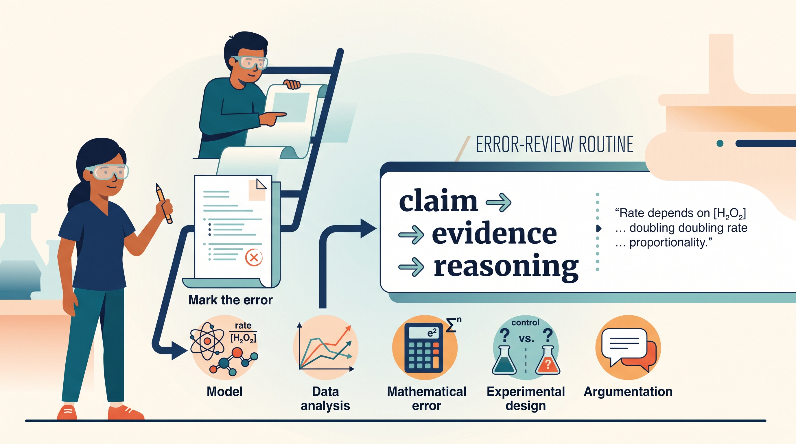
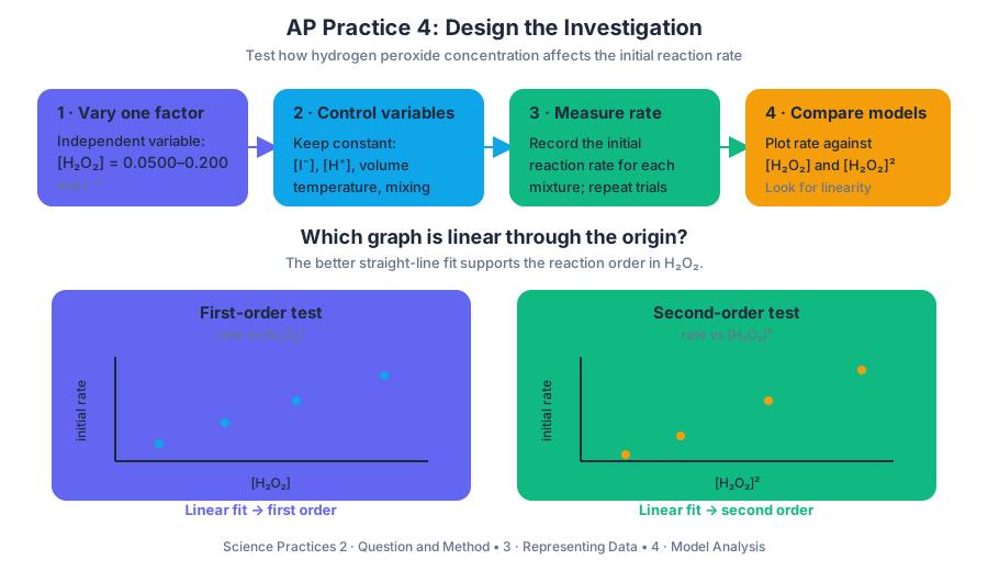
AP Practice 5
A short free-response question rewards selective precision: identify the chemical relationship, show the essential calculation or representation, and connect the result to a defensible explanation.
AP Practice 5
A short free-response question rewards selective precision: identify the chemical relationship, show the essential calculation or representation, and connect the result to a defensible explanation. This practice uses an original equilibrium scenario and emphasizes Science Practice 4: Model Analysis, Science Practice 5: Mathematical Routines, and Science Practice 6: Argumentation.
Task type: Short free-response question
Recommended timing: about $10$–$12$ minutes. Spend approximately $2$ minutes reading the chemical context, $5$ minutes solving, and $3$–$5$ minutes checking units, signs, significant figures, and whether each explanation actually refers to the data.
Original practice prompt
A sealed container holds the gases $A_2$, $B_2$, and $AB$ at constant temperature. They establish the equilibrium
A_2(g)+B_2(g)\rightleftharpoons 2AB(g)
At equilibrium, the concentrations are
$$ [A_2]=0.40\ \mathrm{M},\qquad [B_2]=0.25\ \mathrm{M},\qquad [AB]=0.60\ \mathrm{M}. $$
(a) Write the equilibrium-constant expression, $K_c$, for the reaction.
(b) Calculate the value of $K_c$.
(c) A quantity of $AB(g)$ is injected into the container. Predict the direction in which the reaction initially proceeds. Justify the prediction using the reaction quotient, $Q_c$, rather than only a verbal statement of Le Châtelier’s principle.
(d) After the system reestablishes equilibrium, is the final value of $K_c$ greater than, less than, or equal to the initial value? Explain.
Worked solution
(a) Constructing the model
For a reaction
aA+bB\rightleftharpoons cC,
the equilibrium expression contains each aqueous or gaseous species raised to the power of its stoichiometric coefficient. Pure solids and pure liquids are omitted; all three species here are gases, so all appear.
$$ K_c=\frac{[AB]^2}{[A_2][B_2]} $$
Rubric-aligned checkpoint: The response must use the correct species, place products over reactants, and apply the coefficient $2$ as an exponent on $[AB]$. Writing $[AB]/([A_2][B_2])$ loses the stoichiometric-power relationship.
(b) Calculating $K_c$
Substitute the equilibrium concentrations:
$$ K_c=\frac{(0.60)^2}{(0.40)(0.25)} $$
$$ K_c=\frac{0.36}{0.10}=3.6 $$
Thus,
$$ \boxed{K_c=3.6} $$
Because the concentrations are measured in $\mathrm{M}$ and the reaction has equal total gaseous stoichiometric amounts on both sides, the numerical value is commonly reported without emphasizing a remaining concentration unit in introductory equilibrium work. The critical AP reasoning is the correct expression and substitution.
Rubric-aligned checkpoint: Earn the calculation credit by showing the expression, substituting the data, and obtaining a numerically consistent result. A bare answer of $3.6$ does not demonstrate whether the equilibrium expression was constructed correctly.
(c) Using $Q_c$ after a disturbance
Immediately after $AB$ is injected, the concentration of $AB$ increases, while the concentrations of $A_2$ and $B_2$ have not yet changed. The system is therefore no longer at equilibrium. Suppose, for illustration, that $[AB]$ temporarily rises to $0.80\ \mathrm{M}$:
$$ Q_c=\frac{(0.80)^2}{(0.40)(0.25)} =\frac{0.64}{0.10}=6.4 $$
The comparison is
$$ Q_c=6.4>K_c=3.6 $$
A value of $Q_c$ greater than $K_c$ means that the mixture contains too much product relative to the equilibrium ratio. The reaction proceeds to the left, consuming $AB$ and forming $A_2$ and $B_2$, until $Q_c$ returns to $K_c$.
$$ \boxed{\text{The reaction initially proceeds toward the reactants.}} $$
Rubric-aligned checkpoint: A complete justification contains both the comparison $Q_c>K_c$ and the chemical consequence: the reverse reaction occurs. “The system shifts left because of Le Châtelier’s principle” identifies the direction but does not use the requested quantitative model.
(d) What happens to $K_c$?
The final value of $K_c$ is equal to the initial value, provided the temperature remains constant:
$$ \boxed{K_{c,\mathrm{final}}=K_{c,\mathrm{initial}}} $$
Adding $AB$ changes the concentrations and therefore changes $Q_c$, but it does not change the equilibrium constant. For this reaction, temperature is the condition that determines $K_c$. The reaction shifts until the concentrations once again satisfy the same value of $K_c$.
This distinction is central:
| Quantity | Changes when $AB$ is added? | Meaning |
|---|---|---|
| $Q_c$ | Yes | Ratio calculated from the current, possibly nonequilibrium concentrations |
| $K_c$ | No, if temperature is constant | Ratio required at equilibrium |
Common misconception check
Misconception: “If the reaction shifts left, $K_c$ decreases.” The shift changes the concentrations, not the temperature. Therefore the system changes $Q_c$ until it matches the unchanged $K_c$.
Misconception: “A larger $Q_c$ means a faster reaction.” $Q_c$ indicates the reaction’s direction relative to equilibrium; it does not by itself provide a rate. Kinetics and equilibrium answer different questions: how fast? versus which composition is favored?
Error-review routine
After completing the response, mark each error as one of four types:
- Model error: incorrect species, exponents, or placement in the $K_c$ expression.
- Mathematical error: substitution, arithmetic, or algebra mistake.
- Direction error: incorrect interpretation of $Q_c$ compared with $K_c$.
- Argumentation error: a conclusion is stated without chemical evidence.
Rewrite only the missed part, using the sentence pattern:
“Because $Q_c$ is [greater than/equal to/less than] $K_c$, the reaction proceeds [left/right/no net direction] to [consume/form] ________, restoring the equilibrium ratio.”
Retrieval check: If a reaction mixture has $Q_c<K_c$, which side is initially favored, and what happens to $Q_c as equilibrium is restored?
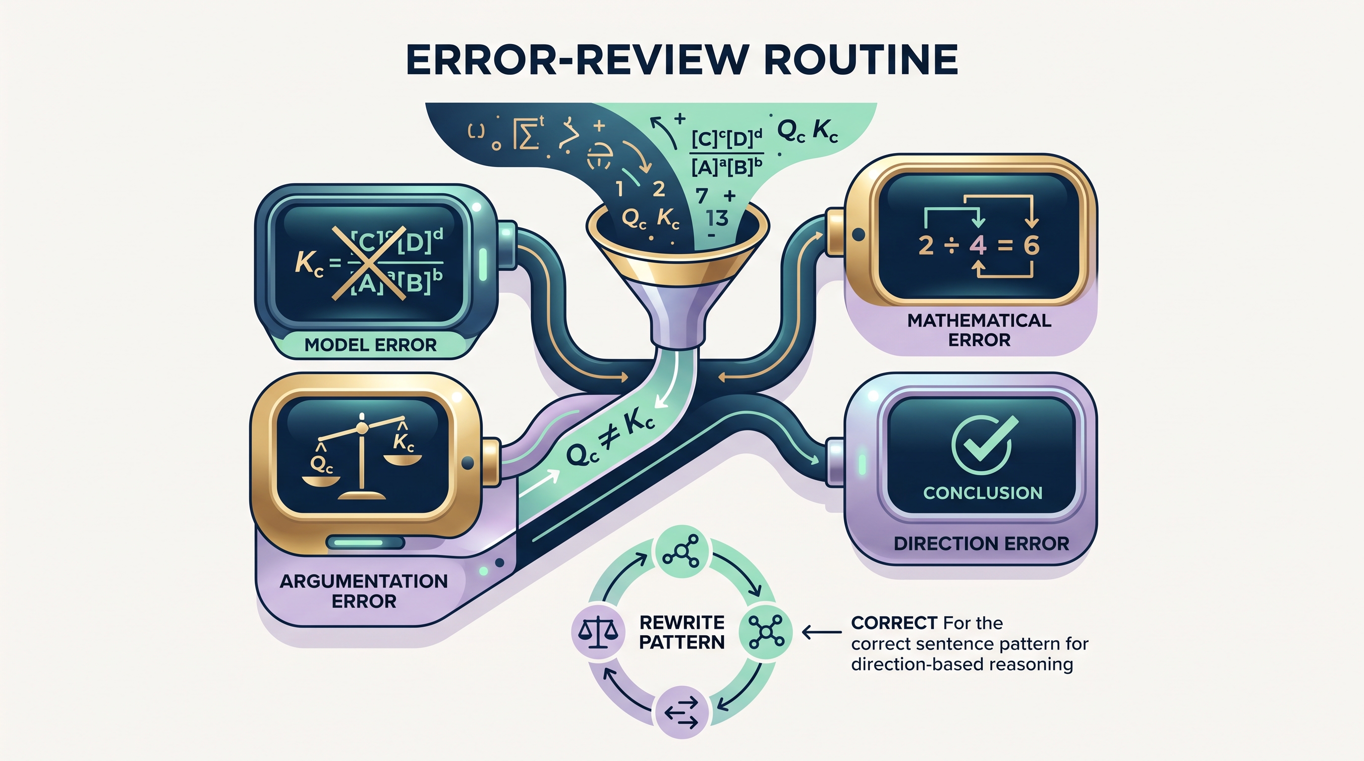
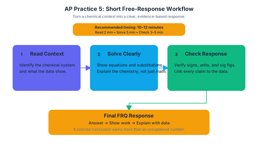
AP Practice 6
A strong chemistry answer does more than state a number: it connects a representation, a measurement, a calculation, and a defensible scientific claim. This original, unofficial practice set uses a short free-response task built around that chain.
AP Practice 6
A strong chemistry answer does more than state a number: it connects a representation, a measurement, a calculation, and a defensible scientific claim. This original, unofficial practice set uses a short free-response task built around that chain. It emphasizes Science Practice 2: Question and Method, Science Practice 3: Representing Data and Phenomena, Science Practice 4: Model Analysis, Science Practice 5: Mathematical Routines, and Science Practice 6: Argumentation.
Task profile: evidence-based short free response
Treat this as a timed short free-response task. Spend approximately $10$–$12$ minutes reading the experimental context, organizing calculations, and writing explanations. A concise response earns more than a long response that hides its claim.
Original practice question: Determining an unknown concentration
A student investigates the concentration of a blue copper(II) ion solution, $Cu^{2+}(aq)$, using visible-light spectroscopy. The student prepares several solutions from a stock solution and measures the absorbance of each solution at the wavelength where the solution absorbs most strongly.
The relevant relationship is the Beer–Lambert law:
$$ A = \varepsilon b c $$
where $A$ is absorbance, $\varepsilon$ is the molar absorptivity, $b$ is the path length of the cuvette, and $c$ is the concentration of the absorbing species. The cuvette path length is constant for all measurements.
| Concentration of $Cu^{2+}$, $c$ ($mol,L^{-1}$) | Absorbance, $A$ |
|---|---|
| $0.0100$ | $0.118$ |
| $0.0200$ | $0.241$ |
| $0.0300$ | $0.356$ |
| $0.0400$ | $0.481$ |
An unknown sample has an absorbance of $0.302$.
(a) Identify the independent variable and dependent variable in the investigation.
(b) Use the data to estimate the concentration of the unknown sample.
(c) A student claims that the solution with concentration $0.0400\ mol,L^{-1}$ contains twice as many copper(II) ions as the solution with concentration $0.0200\ mol,L^{-1}$. Evaluate the claim.
(d) Identify one experimental condition that should be kept constant and explain why changing it could affect the absorbance.
Worked reasoning
(a) Variables
The independent variable is the concentration of $Cu^{2+}$, because the student deliberately changes it. The dependent variable is absorbance, because it is measured in response to the concentration.
Scoring logic: Name what is deliberately changed and what is measured. Do not identify “the solution” as a variable; that description is too vague.
(b) Interpolating from the calibration data
The unknown absorbance, $0.302$, lies between the absorbances for $0.0200\ mol,L^{-1}$ and $0.0300\ mol,L^{-1}$. Therefore, interpolate between those two points rather than extrapolating beyond the measured range.
Using a linear approximation:
$$ \frac{0.302-0.241}{0.356-0.241}
\frac{c-0.0200}{0.0300-0.0200} $$
$$ \frac{0.061}{0.115}
\frac{c-0.0200}{0.0100} $$
$$ c
0.0200 + \left(\frac{0.061}{0.115}\right)(0.0100) $$
$$ c \approx 0.0253\ mol,L^{-1} $$
The estimated concentration is therefore approximately $0.025\ mol,L^{-1}$.
Scoring logic: A complete mathematical response identifies the two surrounding data points, uses the trend represented by the data, and reports a concentration with appropriate units. A calculator-only answer without a visible setup may not demonstrate the reasoning required by Science Practice 5: Mathematical Routines.
(c) Connecting concentration to particle number
The claim is correct only if the two samples have equal volume. Concentration describes the number of moles per unit volume:
$$ c=\frac{n}{V} $$
The concentration ratio is
$$ \frac{0.0400}{0.0200}=2.00 $$
Thus, equal volumes of the two solutions contain a $2.00$ ratio of moles, and therefore a $2.00$ ratio of $Cu^{2+}$ ions. If the volumes differ, the total numbers of ions cannot be compared from concentration alone.
This is an application of Science Practice 6: Argumentation: the claim must include the condition that makes the evidence sufficient.
(d) Controlling experimental conditions
The wavelength should remain constant. Absorbance depends on how strongly the substance absorbs the selected wavelength; changing the wavelength changes $\varepsilon$ and can change the measured absorbance even when the concentration is unchanged. Other valid controls include cuvette path length, solvent, temperature, and instrument blanking.
Common misconception check
Misconception: “Absorbance is the concentration.” Absorbance is a measured response related to concentration through $A=\varepsilon bc$. It is proportional to concentration only when the wavelength, path length, chemical identity, and relevant experimental conditions are held constant.
Misconception: “A trend line proves every sample follows the model perfectly.” The data support an approximately linear relationship, but measurement uncertainty and preparation error remain possible. A scientifically careful answer says “estimated” or “approximately,” especially when interpolating.
Error-review routine
After completing the task, classify each missed point:
- Representation error: Did you misread the table or relationship?
- Mathematical error: Did you use the wrong quantities, units, or equation?
- Method error: Did you confuse an independent variable with a control?
- Reasoning error: Did your conclusion omit a condition or fail to connect evidence to the claim?
Then rewrite only the weakest response in one or two precise sentences. The goal is not merely to obtain $0.025\ mol,L^{-1}$; it is to make the data, model, calculation, and conclusion agree.

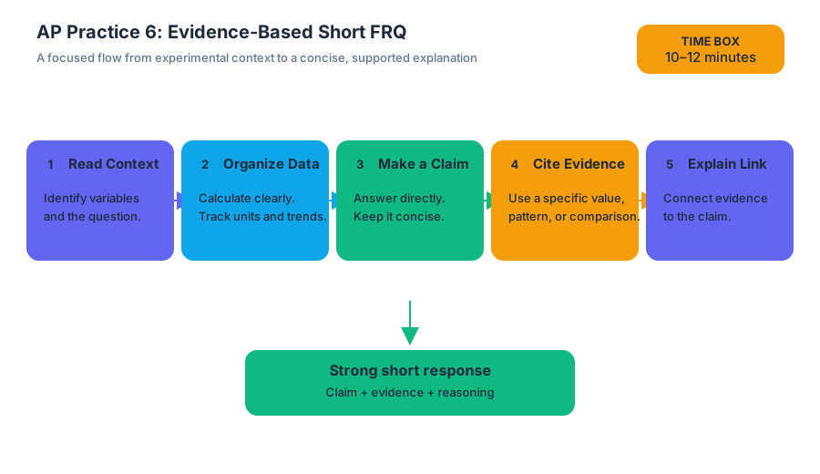
Source Materials
- AP Chemistry Course and Exam Description
- AP Chemistry Course and Exam Description Clarifications and Corrections
- AP Chemistry Course Overview
- AP Chemistry Course at a Glance
- AP Chemistry Course at a Glance Poster
- Adopt AP Chemistry
- AP Chemistry
- AP Chemistry
- Figure — AP Chemistry Course and Exam Description (p. 1)
- Figure — AP Chemistry Course and Exam Description (p. 15)
- continued on next page
- continued on next page
Study AP Chemistry with AI — Free on Lykke
Sign up for free to generate personalized flashcards, quizzes, and study guides from this course. Chat with an AI tutor that knows the material.
Get Started FreeView this course wiki on Lykke · Browse all public course wikis