AP Calculus AB
Institution: MIT
91 study materials · 94 sections
AP Calculus AB students working the current College Board Course and Exam Description, including first-time students with no prior background, plus teachers reviewing the page for CED alignment.; Teach every official CED unit and every numbered topic at topic granularity.; Develop every AP skill / science-practice code explicitly and by name.; Replace description with teaching: worked contextual examples, named misconceptions, and in-flow retrieval checks.; Build an exam-practice unit covering every task type on the current exam.
Course Sections
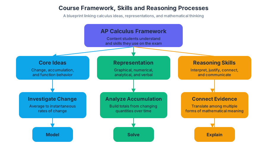
Course Framework, Skills and Reasoning Processes
Key concepts: AP course framework · Course content and skills · Instructional model · Course and exam description · Curriculum transparency · College-level course alignment · AP Course Audit · AP Classroom resources · Student assessment and reporting · Access and readiness for AP coursework
The AP Calculus course framework is the blueprint that identifies the calculus content students must understand and the skills they must be able to use on the AP Exam.
Course Framework, Skills and Reasoning Processes
The AP Calculus course framework is the blueprint that identifies the calculus content students must understand and the skills they must be able to use on the AP Exam.
AP Calculus AB treats calculus as more than a collection of derivative and integral rules. Students investigate how mathematics measures instantaneous change, describes accumulation over time, and analyzes functions through graphical, numerical, analytical, and verbal representations.
The framework as a course blueprint
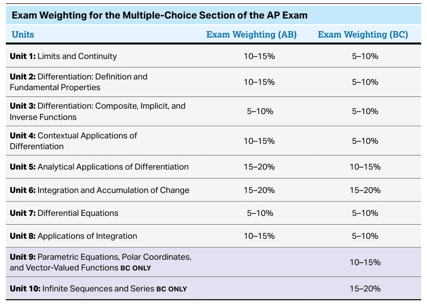
The framework is the heart of the Course and Exam Description. It organizes required content and skills into units that resemble the sequence used in widely adopted college calculus textbooks. This structure gives teachers a coherent progression while leaving room to adjust examples, pacing, readings, and assignments for local needs.
A topic in the framework is best understood as a three-part chain:
| Framework element | Question it answers | Calculus example |
|---|---|---|
| Enduring Understanding | What lasting mathematical idea matters? | A function can describe changing quantities. |
| Learning Objective | What must a student be able to do? | Interpret the derivative in context. |
| Essential Knowledge | What facts and relationships make that action possible? | The derivative gives an instantaneous rate of change. |
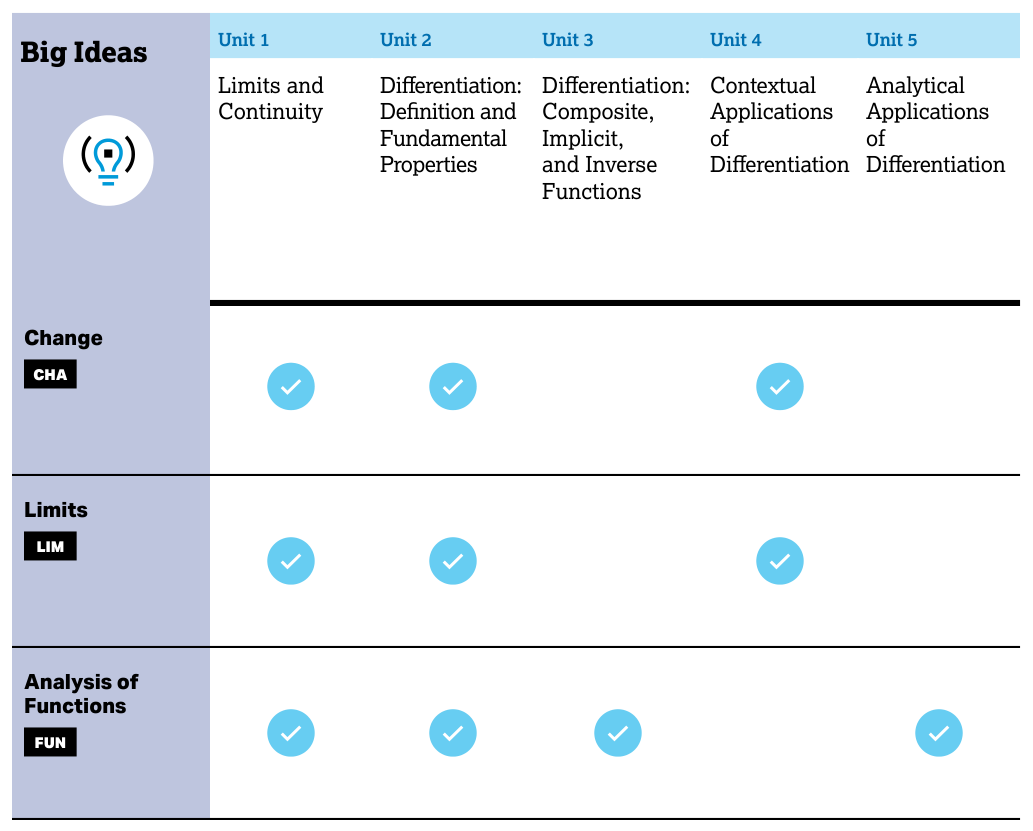
The units therefore should not be taught as isolated boxes. Limits support derivatives; derivatives support applications and differential equations; definite integrals connect rates to accumulated quantities; and representations allow students to move between a graph, table, equation, and explanation without losing the meaning of the mathematics.
The four Mathematical Practices
The AP Calculus framework develops four official reasoning processes, called Mathematical Practice 1—Implementing Mathematical Processes, Mathematical Practice 2—Connecting Representations, Mathematical Practice 3—Justification, and Mathematical Practice 4—Communication and Notation.
Mathematical Practice 1—Implementing Mathematical Processes means selecting and carrying out an appropriate mathematical procedure. A student may evaluate a limit algebraically, differentiate implicitly, construct a Riemann sum, or solve a differential equation. The important question is not merely whether the procedure was remembered, but whether it fits the structure of the problem.
Mathematical Practice 2—Connecting Representations means translating information among equations, graphs, tables, verbal descriptions, and numerical approximations. For example, if a velocity function satisfies $v(t)<0$ on an interval, its graph communicates that position is decreasing, while the integral $\int_a^b v(t),dt$ communicates the net change in position.
Mathematical Practice 3—Justification requires checking conditions and explaining why a conclusion follows. A statement such as “there is a zero” may require continuity and a sign change so that the Intermediate Value Theorem applies. A global-extrema conclusion may require checking endpoints as well as critical points.
Mathematical Practice 4—Communication and Notation requires precise mathematical language, notation, units, and conclusions. A response should distinguish a value from a rate, include units when the context supplies them, and state what a number means rather than leaving an unexplained calculation.
A skill-centered roadmap
All eight units use all four practices, but their emphasis shifts as the mathematics develops:
- Units 1–3: Limits and Differentiation lean heavily on Mathematical Practice 1 and Mathematical Practice 2 as students build symbolic procedures and connect them to graphs and numerical evidence.
- Units 4–5: Contextual and Analytical Applications of Differentiation place greater weight on Mathematical Practice 3 and Mathematical Practice 4 because interpretations, conditions, and explanations determine whether an answer is valid.
- Units 6–8: Integration, Differential Equations, and Applications of Integration combine all four practices: students model accumulation, select procedures, interpret signed quantities, and justify conclusions in context.
These practices appear throughout the exam rather than belonging to separate “skill questions.” Multiple-choice questions may ask students to interpret a representation or select a procedure. Free-response questions commonly require a calculation together with a justification, an interpretation with units, or a connection between a function and its derivative or integral.
Instructional model and public transparency
The instructional model shows possible ways to integrate AP resources across the year so that conceptual understanding and mathematical skills grow together. A typical sequence might introduce a unit, use graphical or numerical exploration, practice analytical procedures, apply the ideas to a real situation, and then use formative evidence to decide what needs reinforcement.
AP Classroom supports this cycle with assignments, multiple-choice questions with rationales, free-response questions, scoring information, and Progress Checks. The Reports feature displays student results across assignment types and helps teachers identify class trends rather than relying only on a single test score.
Public course frameworks and sample assessments promote curriculum transparency: students, families, teachers, and schools can see the mathematical expectations before instruction begins. Transparency does not require every classroom to look identical; the framework is a shared destination, while teachers retain responsibility for selecting college-level readings, resources, examples, and pacing.
Course Audit, syllabus evidence, and access
The AP Course Audit requires an AP teacher and the school principal or designated administrator to confirm awareness and understanding of the curricular and resource requirements. A syllabus or course outline must show how those requirements are met, including access to a college-level calculus textbook, coverage of the AP units and big ideas, mathematical practices, graphing-calculator opportunities, and real-world applications.
The framework also supports access and readiness. AP encourages educators to invite students from groups underrepresented in AP and to use Pre-AP coursework to build preparation. The central principle is that access should expand while students receive the conceptual, procedural, representational, and communication support needed for college-level work.
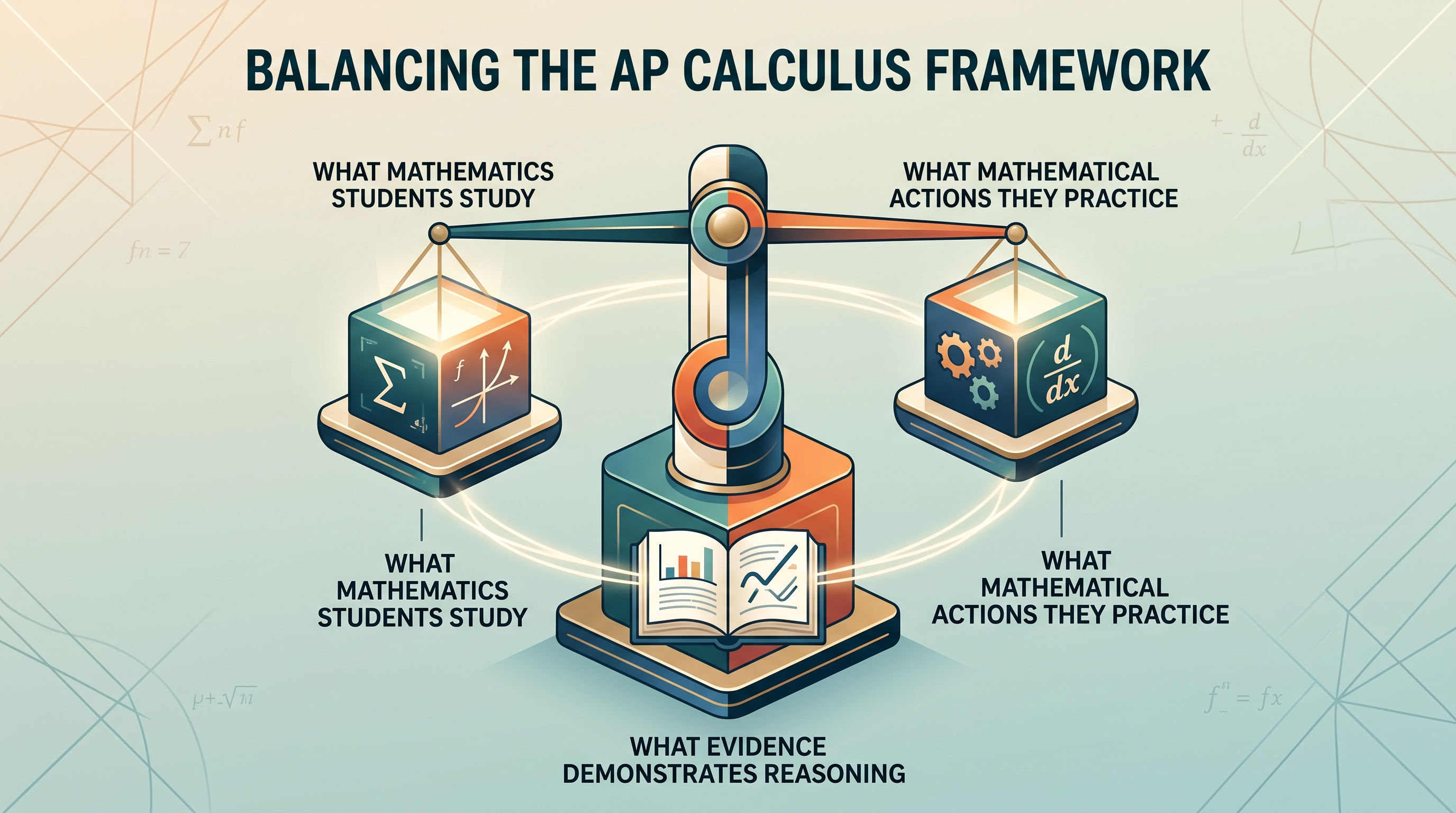
A strong AP Calculus course aligns three things: what mathematics students study, what mathematical actions they practice, and what evidence demonstrates that they can reason with the mathematics.
Retrieval check: A student finds $\int_0^5 v(t),dt=18$ and writes, “The object travels $18$ meters.” Which practice should prompt the correction first? The key issue is Mathematical Practice 4—Communication and Notation, supported by Mathematical Practice 2—Connecting Representations: the integral gives net change in position, not necessarily total distance traveled.

1.1 Introducing Calculus: Can Change Occur at an Instant?
Key concepts: Calculus as the study of change · Whether change can be described at an instant
How calculus turns average rates over shrinking intervals into a rate of change at a single instant.
1.1 Introducing Calculus: Can Change Occur at an Instant?
A speedometer reports a car’s speed at an instant, even though speed is fundamentally a comparison of distance traveled over time. Calculus makes that comparison precise: it studies change, including how a quantity changes at one exact moment.
From average change to change at an instant
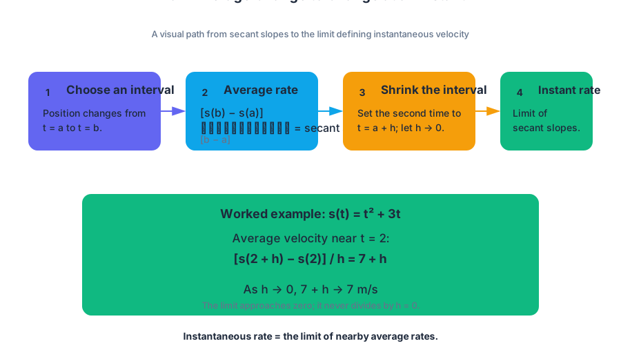
Suppose a cyclist’s position is $s(t)$ meters after $t$ seconds. Over the interval from $t=a$ to $t=b$, the average rate of change is
$$ \frac{s(b)-s(a)}{b-a}. $$
Geometrically, this is the slope of the secant line joining two points on the graph of $s$. It tells us what happened across an interval, not exactly what happened at its endpoint or midpoint.
To estimate the cyclist’s velocity at the instant $t=a$, choose a nearby time $t=a+h$. The corresponding average velocity is
$$ \frac{s(a+h)-s(a)}{h}. $$
As $h$ becomes increasingly close to $0$, the second point on the graph moves toward the first. If the secant slopes approach one definite number, that number describes the cyclist’s instantaneous rate of change.
For example, let $s(t)=t^2+3t$ meters. The average velocity from $t=2$ to $t=2+h$ is
$$ \frac{s(2+h)-s(2)}{h}
\frac{(2+h)^2+3(2+h)-(2^2+3\cdot2)}{h}. $$
Simplifying,
$$ \frac{4+4h+h^2+6+3h-10}{h}
\frac{7h+h^2}{h}
7+h. $$
As $h\to0$, $7+h\to7$. Thus the velocity at $t=2$ is $7$ meters per second. The calculation does not divide by $0$; it examines values of $h$ near $0$ and identifies the value the rates approach.
Key idea: An instantaneous rate is not an average rate over a zero-length interval. It is the limit of average rates over intervals whose lengths approach zero.
Reasoning and representation
This topic is CHA 1.1 Introducing Calculus: Can Change Occur at an Instant?, and it leans on Mathematical Practice 2—Connecting Representations: the same idea appears as a secant slope on a graph, a difference quotient in symbols, and an average velocity with units in words. A strong answer connects those views and states the rate with its units, rather than reporting a bare number.
Retrieval check: For $s(t)=t^2+3t$, the average velocity from $t=2$ to $t=2+h$ simplified to $7+h$. What is the average velocity when $h=0.1$, and what value do these averages approach as $h$ shrinks? Why is that different from substituting $h=0$ at the start?
1.2 Defining Limits and Using Limit Notation
Key concepts: The concept of a limit · Limit notation · Evaluating limits graphically · Evaluating limits numerically · Evaluating limits analytically · Evaluating limits verbally · Using limits to analyze functions and justify conclusions · The connection between limits and continuity
What a limit means, how to write it, and how to read one from a graph, a table or algebra, including when it differs from the function's value.
1.2 Defining Limits and Using Limit Notation
Topic 1.1 found an instantaneous velocity by watching what average velocities approach as the time interval shrinks. That idea of approaching a value, without needing to arrive at it, is the limit. This page gives it a precise meaning and the notation used for it everywhere else in the course.
What a limit means
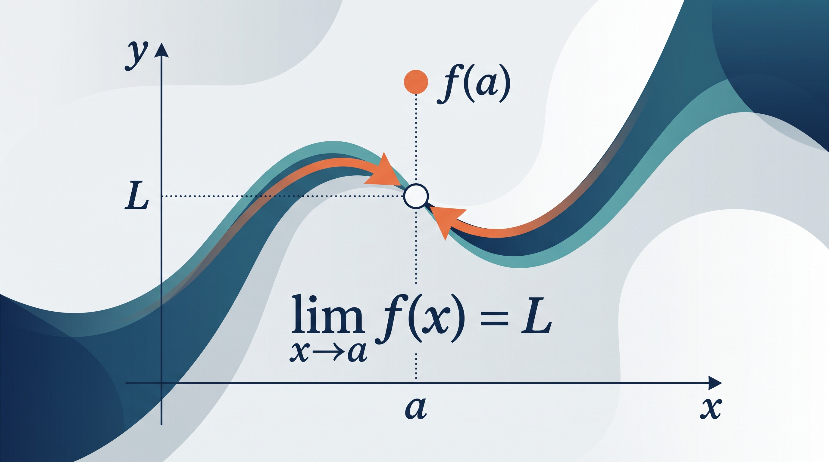
A limit describes the value that a function approaches as its input approaches a particular number. The notation
$$ \lim_{x\to a}f(x)=L $$
means that $f(x)$ approaches $L$ as $x$ approaches $a$.
The arrow in $x\to a$ describes the input’s motion; it does not require $x=a$. This distinction matters because the function may be undefined at $a$, or its actual value $f(a)$ may differ from the value approached nearby.
Consider
$$ f(x)=\frac{x^2-4}{x-2}. $$
At $x=2$, the expression is undefined because its denominator is $0$. For $x\ne2$, factor and simplify:
$$ f(x)=\frac{(x-2)(x+2)}{x-2}=x+2. $$
Therefore,
$$ \lim_{x\to2}\frac{x^2-4}{x-2}
\lim_{x\to2}(x+2)
4, $$
even though $f(2)$ does not exist.
Reading a limit from representations
A graph gives a visual limit procedure: locate $x=a$, then inspect the $y$-values the curve approaches as $x$ moves toward $a$ from the left and from the right. If both sides approach the same number $L$, then $\lim_{x\to a}f(x)=L$; if they approach different values, the two-sided limit does not exist.
A removable hole illustrates the distinction clearly: a curve may approach $y=4$ from both directions while displaying an open circle at $(2,4)$ and a filled point elsewhere—or no filled point at all. The limit is still $4$ because the limit concerns nearby behavior, not necessarily the point’s plotted value.
Nearby numerical values can also support a limit estimate. The reliable question is not “What is the value at $x=a$?” but “What values does $f(x)$ approach when $x$ is chosen increasingly close to $a$?” Extended table-based estimation belongs to Topic 1.4.
Reasoning and representation
These topics emphasize CHA 1.1 Introducing Calculus: Can Change Occur at an Instant? and LIM 1.2 Defining Limits and Using Limit Notation, each associated with Mathematical Practice 2—Connecting Representations. A strong conclusion connects a graphical, numerical, analytical, or verbal observation rather than reporting an unsupported number.
The work also uses Mathematical Practice 1—Implementing Mathematical Processes, when algebraic limit properties or simplification are selected; Mathematical Practice 3—Justification, when left- and right-hand behavior is checked; and Mathematical Practice 4—Communication and Notation, when the limit is written with correct symbols, units, and a clear interpretation. When a calculator is used for a numerical estimate, keep appropriate precision during computation and round the final reported value appropriately.
Misconception check — “The limit equals $f(a)$.”
Not always. The limit is the value approached near $a$; $f(a)$ is the function’s actual assigned value at $a$. They are equal only when the function is defined there with that same value.
Retrieval check: If a graph approaches $y=-3$ from both sides as $x\to5$, but the filled point at $x=5$ has height $2$, state $\lim_{x\to5}f(x)$ and $f(5)$. Why are the two answers different?
1.3 Estimating Limit Values from Graphs
Key concepts: Estimating limit values from graphs · Limit notation · The behavior of a function f as x approaches a particular x-value · Connecting graphical, numerical, analytical, and verbal representations · Identifying mathematical information from representations · Reading function values such as f(6) and f(-6) from a graph · Precise mathematical communication and notational fluency
How to read a limit off a graph by tracing the curve toward the target input from both sides, and why the filled dot at that input does not decide the limit.
1.3 Estimating Limit Values from Graphs
A limit can be estimated without knowing the exact value of a function at the target input: it describes the height that $f(x)$ approaches as $x$ gets close to that input. Graphs show this approach visually; tables show it numerically.
Reading a limit from a graph
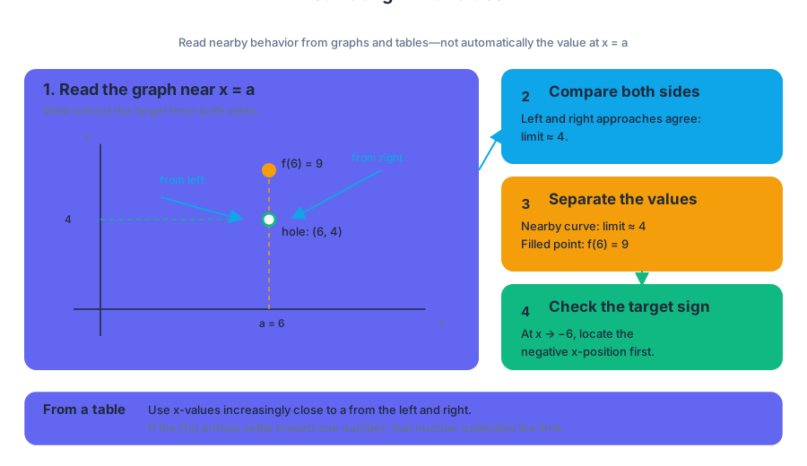
To estimate $\displaystyle \lim_{x\to a}f(x)$, focus on the behavior of the curve near $x=a$, not automatically on the point plotted at $x=a$. Imagine sliding along the curve from the left and from the right. If both sides approach the same $y$-value, that common value is the estimated limit.
For example, suppose a graph has a hole in the curve at $(6,4)$, while a filled point appears at $(6,9)$. The nearby curve approaches $4$ from both sides. Therefore,
$$ \lim_{x\to 6}f(x)\approx 4, $$
even though
$$ f(6)=9. $$
The limit records nearby behavior; the function value records the actual defined output at the target input.
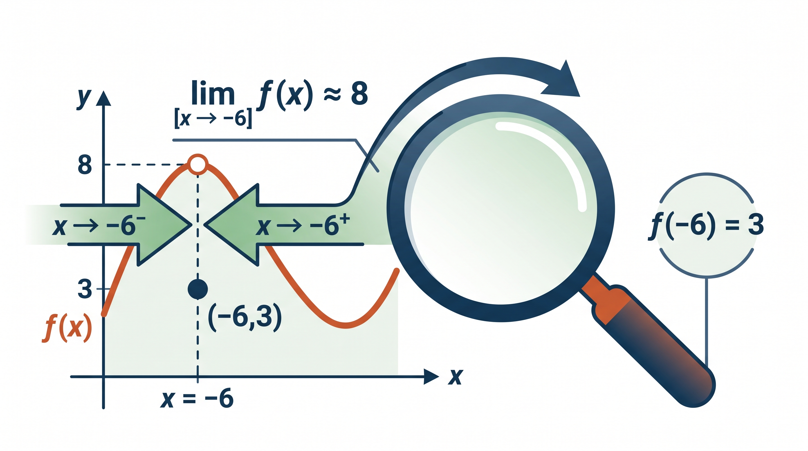
A negative target input must be read just as carefully. Suppose the graph contains a filled point at $(-6,3)$, but the curve on either side of $x=-6$ approaches $7$. Then
$$ f(-6)=3 $$
but
$$ \lim_{x\to -6}f(x)\approx 7. $$
The minus sign in $x\to -6$ identifies the horizontal location being approached. It is not part of the resulting $y$-value.
Graph-reading procedure
- Locate the target input $x=a$, including its sign.
- Trace the curve toward $x=a$ from the left.
- Trace the curve toward $x=a$ from the right.
- Compare the two nearby heights.
- Report the common height, if one exists, using $\displaystyle \lim_{x\to a}f(x)$ notation.
When a graph gives no two-sided limit
The two-sided limit does not exist when the left-hand and right-hand approaches do not agree. A graph may also fail to produce a finite limit if the function grows without bound near the target or oscillates indefinitely.
Named misconception — “The limit is the filled dot.” A filled dot tells you $f(a)$, but it may have no connection to the limit if the surrounding curve approaches a different height. Conversely, an open circle does not mean the limit is nonexistent; the curve may approach the hole from both sides perfectly consistently.
Connecting representations
The same limit may be represented graphically, numerically, analytically, or verbally:
| Representation | Information |
|---|---|
| Graphical | Both branches approach the height $4$ near $x=2$. |
| Numerical | Table values approach $4$ from the left and right. |
| Analytical | $\displaystyle \lim_{x\to 2}f(x)\approx4$. |
| Verbal | “As $x$ gets close to $2$, $f(x)$ gets close to $4$.” |
This cross-checking is Connecting Representations, Skill 2.B: Identify mathematical information from graphical, numerical, analytical, and/or verbal representations. A calculator can zoom, generate tables, or evaluate nearby inputs, but the reasoning remains the same: identify the target input, inspect both directions, and determine whether the outputs approach one common value.
Limit or function value?
Retrieval check: A graph has a filled point at $(-6,3)$, while the curve approaches $8$ from both sides of $x=-6$. State both quantities.
The answer is
$$ f(-6)=3 \qquad\text{and}\qquad \lim_{x\to -6}f(x)\approx8. $$
1.4 Estimating Limit Values from Tables
Key concepts: Estimating limit values from tables · Limit notation · The behavior of a function f as x approaches a particular x-value · Connecting graphical, numerical, analytical, and verbal representations · Identifying mathematical information from representations · Determining whether a limit exists from a table · Using tables of values to investigate limits · Precise mathematical communication and notational fluency
How to estimate a limit from a table of values approaching the target from both sides, how to spot a limit that does not exist, and how far a rounded table can be trusted.
1.4 Estimating Limit Values from Tables
A graph shows a limit as a height the curve heads toward; a table shows the same approach in numbers. When only values are available—measured data, a calculator's table feature, or an exam question with no graph or formula—the limit is estimated from how the outputs behave as the inputs close in on the target from both sides.
Estimating a limit from a table
A numerical table should contain $x$-values increasingly close to the target $a$ from both directions. The corresponding $f(x)$-values reveal whether the outputs settle toward one common number.
Consider the following original data:
| $x$ approaching $2$ from the left | $f(x)$ | $x$ approaching $2$ from the right | $f(x)$ |
|---|---|---|---|
| $1.5$ | $4.10$ | $2.5$ | $3.90$ |
| $1.9$ | $4.01$ | $2.1$ | $3.99$ |
| $1.99$ | $4.001$ | $2.01$ | $3.999$ |
The values on both sides approach $4$. Thus,
$$ \lim_{x\to 2}f(x)\approx 4. $$
The table does not need to contain $x=2$ itself. In fact, the function might be undefined there; the limit can still exist.
A table showing that the limit does not exist
Now compare a table whose left and right outputs approach different numbers:
| $x$ approaching $0$ from the left | $f(x)$ | $x$ approaching $0$ from the right | $f(x)$ |
|---|---|---|---|
| $-0.5$ | $2.4$ | $0.5$ | $5.6$ |
| $-0.1$ | $2.08$ | $0.1$ | $5.92$ |
| $-0.01$ | $2.008$ | $0.01$ | $5.992$ |
From the left, $f(x)$ approaches $2$. From the right, $f(x)$ approaches $6$. Because these one-sided trends disagree,
$$ \lim_{x\to 0}f(x) $$
does not exist. The correct conclusion is not an average such as $4$; a two-sided limit requires agreement between both directions.
Connecting representations
The same limit may be represented graphically, numerically, analytically, or verbally:
| Representation | Information |
|---|---|
| Graphical | Both branches approach the height $4$ near $x=2$. |
| Numerical | Table values approach $4$ from the left and right. |
| Analytical | $\displaystyle \lim_{x\to 2}f(x)\approx4$. |
| Verbal | “As $x$ gets close to $2$, $f(x)$ gets close to $4$.” |
This cross-checking is Connecting Representations, Skill 2.B: Identify mathematical information from graphical, numerical, analytical, and/or verbal representations. A calculator can zoom, generate tables, or evaluate nearby inputs, but the reasoning remains the same: identify the target input, inspect both directions, and determine whether the outputs approach one common value.
Misconception check and retrieval
Rounded-table caution: Nearby values such as $3.99$ and $4.01$ suggest a limit near $4$, but a short table is evidence, not proof. Use closer inputs when possible, and do not confuse small numerical differences caused by rounding with genuinely different one-sided behavior.
Retrieval check: Near $x=3$, a table gives $f(2.9)=6.8$, $f(2.99)=6.98$ and $f(2.999)=6.998$ from the left, and $f(3.1)=7.2$, $f(3.01)=7.02$ and $f(3.001)=7.002$ from the right. Estimate $\lim_{x\to3}f(x)$. Both columns settle toward $7$, so the limit is approximately $7$, whether or not $f(3)$ is defined.
1.5 Determining Limits Using Algebraic Properties of Limits
Key concepts: Algebraic properties of limits · Limit theorems · Limits of sums, products, quotients, and composite functions · Connecting graphical, numerical, and algebraic representations of limits · Evaluating limits across multiple representations · Determining limits of analytically expressed functions · Using algebra rather than technology to determine limits · Skill 1.E: applying algebraic properties of limits
The limit laws for sums, differences, products, quotients, constant multiples and composites, used to build a limit from limits that are already known.
1.5 Determining Limits Using Algebraic Properties of Limits
When two quantities approach predictable values, their sum, difference, product, or quotient usually approaches the corresponding combination of those values. The limit laws turn that idea into a reliable calculation procedure—and algebraic manipulation rescues problems where direct substitution produces an indeterminate form.
The limit laws: combine known behavior
The enduring understanding LIM-1, “Reasoning with definitions, theorems, and properties can be used to justify claims about limits,” is applied here through learning objective LIM-1.D, “Determine the limits of functions using limit theorems.” Essential knowledge LIM-1.D.1 recognizes that one-sided limits can be determined analytically or graphically, while LIM-1.D.2 states that limits of sums, differences, products, quotients, and composite functions can be found using limit theorems.
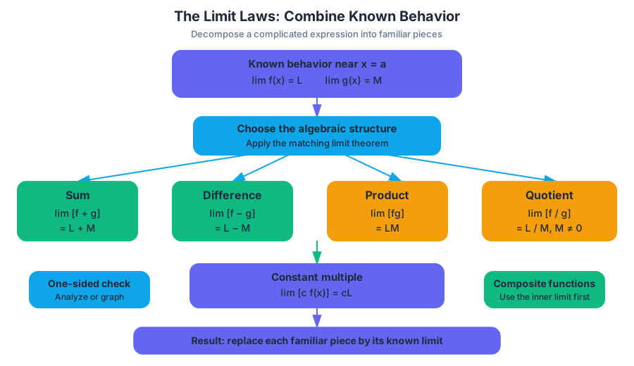
Suppose $\lim_{x\to a}f(x)=L$ and $\lim_{x\to a}g(x)=M$. Then the basic algebraic properties of limits are
$$ \lim_{x\to a}[f(x)+g(x)]=L+M, $$
$$ \lim_{x\to a}[f(x)-g(x)]=L-M, $$
$$ \lim_{x\to a}[f(x)g(x)]=LM, $$
and, provided $M\ne 0$,
$$ \lim_{x\to a}\frac{f(x)}{g(x)}=\frac{L}{M}. $$
A constant multiple behaves as expected:
$$ \lim_{x\to a}[cf(x)]=cL. $$
These rules allow a complicated expression to be decomposed into familiar pieces.
Worked example: a rate assembled from several effects
A sensor models the combined signal near time $t=2$ by
$$ S(t)=t^3+4\sin t-\frac{6}{t+1}. $$
Because polynomials, sine, and rational functions have limits found by direct substitution at $t=2$, apply the limit laws term by term:
$$ \begin{aligned} \lim_{t\to2}S(t) &=\lim_{t\to2}t^3+4\lim_{t\to2}\sin t -6\lim_{t\to2}\frac{1}{t+1}\ &=2^3+4\sin(2)-\frac{6}{3}\ &=6+4\sin(2). \end{aligned} $$
The limit exists even though the expression contains several different operations. The important move is not “substitute everywhere automatically,” but identify the structure and apply a theorem legally.
Composite functions: the outside function must behave well
A composite function applies one function to the output of another, such as $F(x)=\sqrt{5x+4}$. If $\lim_{x\to a}g(x)=M$ and the outer function $f$ is continuous at $M$, then
$$ \lim_{x\to a}f(g(x))=f(M). $$
For example,
$$ \lim_{x\to1}\sqrt{5x+4} =\sqrt{5(1)+4}=3. $$
The condition matters: if the outer function has a break at the approaching value, direct substitution may not be justified.
Multiple representations and an important cancellation
Limit reasoning may combine a graph, a table, a symbolic formula, and verbal information. For example, suppose a graph shows $\lim_{x\to2}f(x)=5$, a table indicates $\lim_{x\to2}g(x)=-1$, and $h(x)=f(x)g(x)$. Then the product law gives
$$ \lim_{x\to2}h(x)=5(-1)=-5. $$
The representations are different descriptions of the same local behavior; the algebraic theorem connects them.
A subtle exception prevents an incorrect “reverse” conclusion. The limit of $f+g$ can exist even when the individual limits do not. Let
$$ f(x)=\sin\left(\frac{1}{x-a}\right), \qquad g(x)=-\sin\left(\frac{1}{x-a}\right). $$
Neither limit exists as $x\to a$, because each function oscillates indefinitely. Yet
$$ f(x)+g(x)=0 $$
for every $x\ne a$, so
$$ \lim_{x\to a}[f(x)+g(x)]=0. $$
The limit laws tell us how to combine existing limits; they do not say that existence of a combined limit requires existence of every separate limit.
AP skill alignment: Topic 1.5 develops Skill 1.E: Apply appropriate mathematical rules or procedures, with and without technology. Topic 1.6 develops Skill 1.C: Identify an appropriate mathematical rule or procedure based on the classification of a given expression. Supporting work also uses Skill 2.B: Identify mathematical information from graphical, numerical, analytical, and/or verbal representations when data from different representations must be connected.
Retrieval check
Suppose $\lim_{x\to3}f(x)=2$ and $\lim_{x\to3}g(x)=-5$. Evaluate $\lim_{x\to3}[f(x)g(x)+4f(x)]$ and name each law you use. The product, constant-multiple and sum laws give $2(-5)+4(2)=-2$.

1.6 Determining Limits Using Algebraic Manipulation
Key concepts: Determining limits using algebraic manipulation · Determining limits of analytically expressed functions · Using algebra rather than technology to determine limits · Skill 1.C: selecting appropriate algebraic manipulation procedures
What to do when substitution gives 0/0: factor and cancel, or rationalize with a conjugate, to reach an equivalent expression whose limit can be evaluated.
1.6 Determining Limits Using Algebraic Manipulation
Direct substitution and the limit laws settle most limits, but some expressions break down at exactly the input being approached: substitution returns $\frac{0}{0}$, and no limit law applies to the expression as written. Algebraic manipulation rewrites the expression into an equivalent form, valid near the target, whose limit can be found directly.
When algebra must come first
For a function given analytically, first try direct substitution. If it produces a real number, the limit laws often finish the problem. If it produces a form such as $\frac{0}{0}$, the expression has not been evaluated; instead, it signals that algebraic manipulation is needed.
Consider the average-cost expression
$$ C(x)=\frac{x^2-9}{x-3}, $$
where $x$ represents production level. At $x=3$, direct substitution gives
$$ \frac{3^2-9}{3-3}=\frac{0}{0}. $$
Factor the numerator:
$$ x^2-9=(x-3)(x+3). $$
For $x\ne3$,
$$ C(x)=\frac{(x-3)(x+3)}{x-3}=x+3. $$
Therefore,
$$ \lim_{x\to3}C(x) =\lim_{x\to3}(x+3)=6. $$
The original function may be undefined at $x=3$, but a limit examines values near $3$, not necessarily the value at $3$.
Rationalizing a difference
A square-root expression can also hide a removable factor. For
$$ \lim_{x\to4}\frac{\sqrt{x}-2}{x-4}, $$
multiplying by the conjugate gives
$$ \frac{\sqrt{x}-2}{x-4}\cdot \frac{\sqrt{x}+2}{\sqrt{x}+2}
\frac{x-4}{(x-4)(\sqrt{x}+2)}
\frac{1}{\sqrt{x}+2}. $$
Thus,
$$ \lim_{x\to4}\frac{\sqrt{x}-2}{x-4}
\frac{1}{2+2} =\frac14. $$
This is algebraic manipulation in action: rewrite the expression into an equivalent form on a punctured neighborhood of the target.
Misconception check
Misconception: “If substitution gives $\frac00$, the limit is zero.” The symbol $\frac00$ is not an answer. It means the numerator and denominator both approach zero, so further reasoning—factoring, rationalizing, or another appropriate algebraic procedure—is required.
AP skill alignment: Topic 1.6 develops Skill 1.C: Identify an appropriate mathematical rule or procedure based on the classification of a given expression. Here the classification comes from what direct substitution produces: a real number means the limit laws finish the problem, while $\frac{0}{0}$ calls for factoring, rationalizing, or another rewriting step first.
Retrieval check
Evaluate without technology:
$$ \lim_{x\to1}\frac{x^2-1}{x-1}. $$
Factor first, cancel only for $x\ne1$, and then substitute. The result is
$$ \boxed{2}. $$
1.7 Selecting Procedures for Determining Limits
Key concepts: Selecting an appropriate procedure for determining a limit · Using equivalent expressions to determine limits · Rearranging expressions into equivalent forms before evaluating a limit · Identifying when a theorem or test is appropriate for a limit · Using mathematical characteristics or properties of functions when selecting a procedure
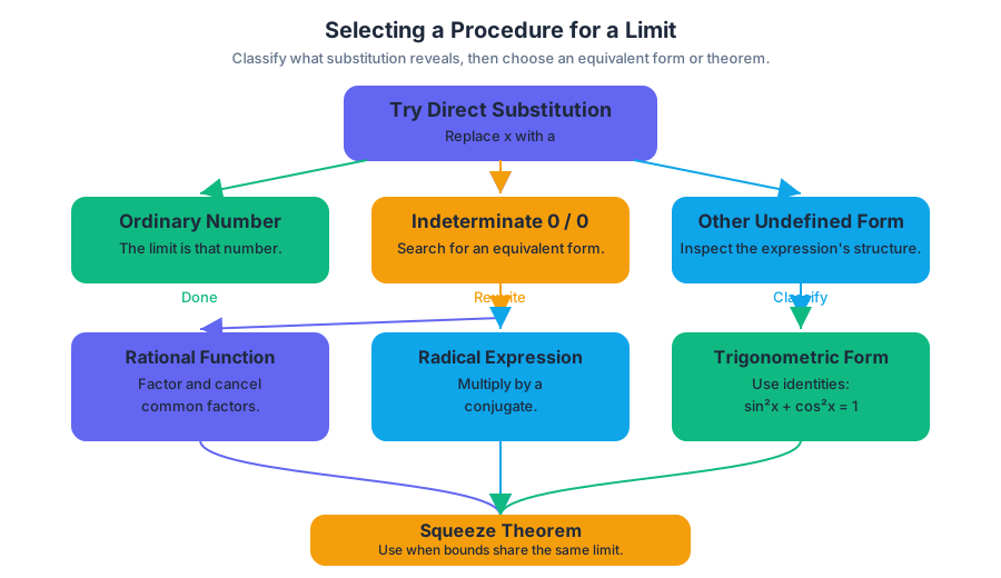
A decision path for limits: try direct substitution, and if it gives 0/0 choose the rewrite that fits the expression, such as factoring, a conjugate, or a trigonometric identity.
1.7 Selecting Procedures for Determining Limits
A limit is often easiest to determine not by calculating harder, but by recognizing what kind of expression is in front of you and choosing a procedure that preserves its behavior.
Enduring Understanding LIM-1: Reasoning with definitions, theorems, and properties can be used to justify claims about limits.
Learning Objective LIM-1.E: Determine the limits of functions using equivalent expressions for the function or the Squeeze Theorem.
Essential Knowledge LIM-1.E.1: It may be necessary or helpful to rearrange expressions into equivalent forms before evaluating limits.
Choosing the procedure
The AP skill emphasized here is 1.C — Identify an appropriate mathematical rule or procedure based on the classification of a given expression. The important decision is not simply “Can I substitute?” but “What does the expression become when I substitute, and what structure does that reveal?”
Use this decision path:
- Try direct substitution. If replacing $x$ with $a$ produces an ordinary real number, that number is the limit.
- If substitution produces $\frac{0}{0}$, the expression is indeterminate, not equal to zero. Search for an equivalent form.
- For rational functions, factor and cancel a common factor when appropriate.
- For radicals, multiply by a conjugate such as $\sqrt{x+c}+d$ or $\sqrt{x+c}-d$.
- For trigonometric expressions, rewrite using identities such as $\sin^2 x+\cos^2 x=1$ or $\tan x=\frac{\sin x}{\cos x}$.
- If the function is trapped between two simpler functions with the same limit, use the Squeeze Theorem.
Equivalent expressions reveal hidden behavior
Two expressions are equivalent on a relevant domain when they produce the same output wherever both are defined. They may look different algebraically, yet have identical limiting behavior near the point of interest. This allows a complicated expression to be replaced by a simpler one before evaluating its limit.
Worked example: a removable algebraic obstruction
Suppose the concentration of a chemical sensor is modeled near $t=3$ by
$$ C(t)=\frac{t^2-9}{t-3}. $$
Direct substitution gives
$$ C(3)=\frac{0}{0}, $$
which tells us only that the original formula cannot be evaluated by substitution. Factor the numerator:
$$ t^2-9=(t-3)(t+3). $$
For $t\ne3$,
$$ C(t)=\frac{(t-3)(t+3)}{t-3}=t+3. $$
Therefore,
$$ \lim_{t\to3}C(t)=\lim_{t\to3}(t+3)=6. $$
The cancellation does not claim that $C(3)$ exists under the original formula. It says that values of $C(t)$ near $t=3$ follow the simpler rule $t+3$, so the limit is $6$.
Radical expressions
For
$$ \lim_{x\to0}\frac{\sqrt{x+4}-2}{x}, $$
substitution again produces $\frac{0}{0}$. Multiply by the conjugate:
$$ \frac{\sqrt{x+4}-2}{x} \cdot \frac{\sqrt{x+4}+2}{\sqrt{x+4}+2}
\frac{x}{x(\sqrt{x+4}+2)}
\frac{1}{\sqrt{x+4}+2}. $$
Thus,
$$ \lim_{x\to0}\frac{\sqrt{x+4}-2}{x}
\frac{1}{4}. $$
Misconception check — “$\frac{0}{0}=0$.” The form $\frac{0}{0}$ is not an answer. It signals that the expression must be classified and transformed, or that another theorem may be needed.
Retrieval check
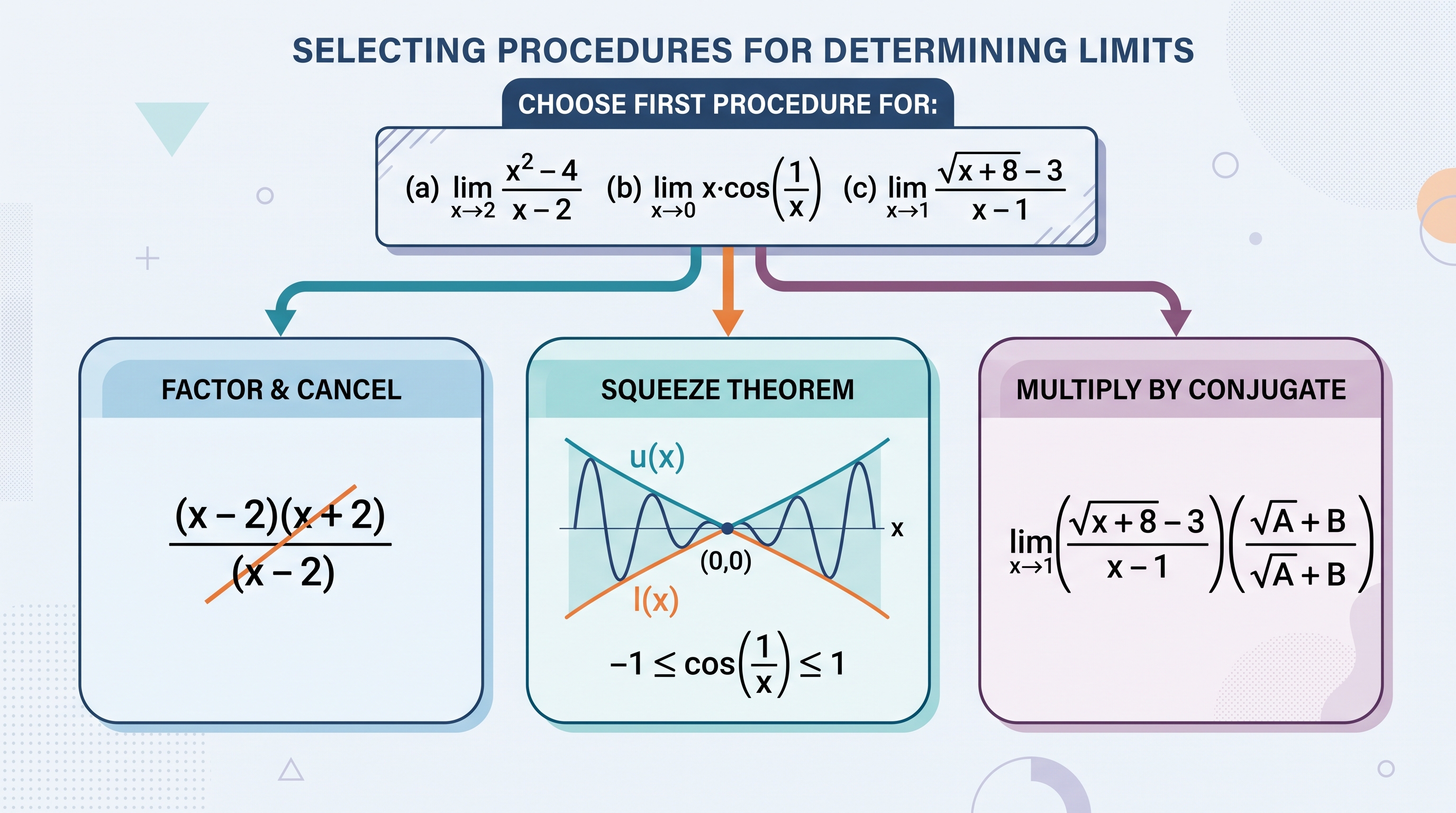
For each expression, name the best first procedure:
(a) $\displaystyle \lim_{x\to2}\frac{x^2-4}{x-2}$;
(b) $\displaystyle \lim_{x\to0}x\cos(1/x)$;
(c) $\displaystyle \lim_{x\to1}\frac{\sqrt{x+8}-3}{x-1}$.
Answers: (a) factor and cancel; (b) use the Squeeze Theorem because $-1\le\cos(1/x)\le1$; (c) multiply by the conjugate. In each case, the procedure follows from the expression’s mathematical characteristics.
1.8 Determining Limits Using the Squeeze Theorem
Key concepts: Determining limits using the Squeeze Theorem · Identifying when a theorem or test is appropriate for a limit
The Squeeze Theorem: finding the limit of a rapidly oscillating expression by trapping it between two simpler functions that approach the same value.
1.8 Determining Limits Using the Squeeze Theorem
Some limits resist every algebraic rewrite: a factor such as $\sin\left(\frac{1}{x}\right)$ oscillates faster and faster near the target, so there is nothing to cancel and substitution is meaningless. The Squeeze Theorem finds such limits indirectly, by trapping the difficult function between two simpler functions that approach the same value.
Enduring Understanding LIM-1: Reasoning with definitions, theorems, and properties can be used to justify claims about limits.
Learning Objective LIM-1.E: Determine the limits of functions using equivalent expressions for the function or the Squeeze Theorem.
The Squeeze Theorem: proving a trapped limit
The Squeeze Theorem determines a limit when a function is bounded above and below by two functions that approach the same value.
If $g(x)\le f(x)\le h(x)$ near $x=a$, and
$$ \lim_{x\to a}g(x)=\lim_{x\to a}h(x)=L, $$
then
$$ \lim_{x\to a}f(x)=L. $$
Worked example: an oscillating sensor signal
A vibration sensor records a signal
$$ s(t)=t^2\sin\left(\frac{1}{t}\right) $$
near $t=0$. The factor $\sin\left(\frac{1}{t}\right)$ oscillates increasingly rapidly, so direct substitution is not useful. But sine always satisfies
$$ -1\le \sin\left(\frac{1}{t}\right)\le1. $$
Because $t^2\ge0$,
$$ -t^2\le t^2\sin\left(\frac{1}{t}\right)\le t^2. $$
Both outside functions approach $0$:
$$ \lim_{t\to0}(-t^2)=0 \qquad\text{and}\qquad \lim_{t\to0}t^2=0. $$
Therefore, the Squeeze Theorem gives
$$ \boxed{\lim_{t\to0}t^2\sin\left(\frac{1}{t}\right)=0}. $$
The oscillation never disappears, but its amplitude is forced into the narrowing interval $[-t^2,t^2]$. The “trap” closes at $0$.
When is the theorem appropriate?
The Squeeze Theorem is appropriate when a difficult factor is bounded and another factor drives the bounds toward one common value. It is especially useful for expressions involving oscillation, such as $\sin(1/x)$ or $\cos(1/x)$, where algebraic rearrangement alone cannot remove the rapid oscillation.
Misconception check — “Rapid oscillation means the limit does not exist.” Oscillation by itself may prevent a limit, but multiplying by a shrinking factor can force the entire expression toward one value. The bounds, not the visual irregularity alone, determine the conclusion.
Retrieval check
Find $\lim_{x\to0}x\cos\left(\frac{1}{x}\right)$. Because $x$ can be negative, bound the product with absolute values: $-|x|\le x\cos\left(\frac{1}{x}\right)\le|x|$. Both $-|x|$ and $|x|$ approach $0$ as $x\to0$, so the Squeeze Theorem gives a limit of $0$.
1.9 Connecting Multiple Representations of Limits
Key concepts: Limits and continuity · Connecting multiple representations of limits · Translating among numerical, graphical, analytical, and verbal representations · Skill 2.C: Connecting representations · Using calculators to evaluate limits, derivatives, or definite integrals · Writing the mathematical setup before reporting a calculator result · AP Calculus AB and BC course framework · Mathematical Practices: Connecting Representations · Limits as a context for integrating multiple representations
How one limit appears as a table, a graph, a formula and a sentence, and how to translate between those representations and check that they agree.
1.9 Connecting Multiple Representations of Limits
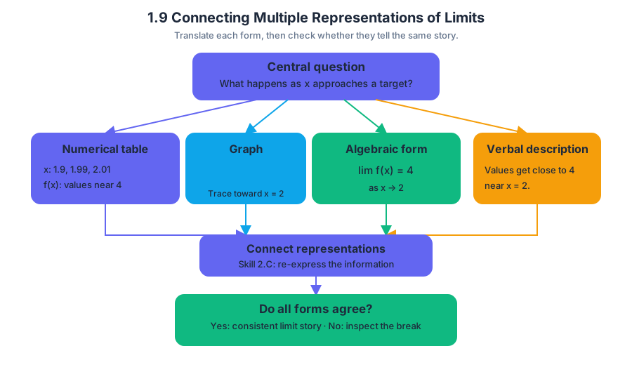
A limit is not trapped inside an equation: the same mathematical behavior can appear as a table of values, a graph, an algebraic expression, or a verbal description. The essential question is: Do all representations tell the same story about what happens as $x$ approaches a target value?
Topic 1.9: Connecting Multiple Representations of Limits emphasizes translating mathematical information among numerical, graphical, analytical, and verbal forms. The associated suggested skill is Skill 2.C: Connecting Representations — “Identify a re-expression of mathematical information presented in a given representation.”
One limit, four mathematical languages
Suppose the temperature near a sensor is modeled by
$$ T(x)=\frac{x^2-9}{x-3}, $$
where $x$ measures a location along a pipe. At $x=3$, the formula is undefined, but for nearby values of $x$,
$$ T(x)=\frac{(x-3)(x+3)}{x-3}=x+3. $$
Thus,
$$ \lim_{x\to 3}T(x)=6. $$
The same conclusion can be translated across representations:
- Analytical: simplify the expression to $x+3$ for $x\ne 3$, then evaluate the limit.
- Numerical: values such as $T(2.9)=5.9$ and $T(3.1)=6.1$ approach $6$.
- Graphical: the graph follows the line $y=x+3$ but has a hole at $(3,6)$.
- Verbal: as the location approaches $3$ from either side, the temperature approaches $6$ units.
The function’s actual value at $x=3$ is not needed to determine the limit. A limit describes nearby behavior, not necessarily the value at the target. This distinction is the bridge between Topic 1.9 and Topic 1.10.
Calculator-supported representations
A graphing calculator can generate a graph, a table, or a numerical limit estimate, making it useful for developing conjectures and checking whether representations agree. It does not replace the mathematical communication that explains what was entered and what the result means.
When a required calculator capability is used, write both the setup and the calculator’s result. For example, to investigate the removable discontinuity above, record
$$ \text{Setup: }\lim_{x\to 3}\frac{x^2-9}{x-3}, \qquad \text{calculator result: }6. $$
If another built-in feature or program produces the result, include the mathematical steps needed to produce it. A decimal by itself is evidence of an output, not evidence of reasoning.
Misconception check: “If $f(a)$ is undefined, the limit does not exist.”
Correction: A function may be undefined at $a$ while its two-sided limit exists. A hole is precisely the graphical signature of this possibility.
Retrieval check
A table gives $f(1.9)=3.8$, $f(1.99)=3.98$, $f(2.01)=4.02$ and $f(2.1)=4.2$. Re-express this numerical information analytically and verbally. The table suggests $\lim_{x\to2}f(x)=4$; in words, as $x$ gets close to $2$ from either side, $f(x)$ gets close to $4$. A graph would show both branches heading toward height $4$ at $x=2$.
1.10 Exploring Types of Discontinuities
Key concepts: Limits and continuity · Exploring types of discontinuities · AP Calculus AB and BC course framework
How to classify a discontinuity as removable, jump or infinite by comparing the one-sided limits with the function's value at the point.
1.10 Exploring Types of Discontinuities
Limits describe where a function is heading near an input; this page uses them to describe what goes wrong at an input where the graph breaks. One example will be reused: the sensor model $T(x)=\frac{x^2-9}{x-3}$ from Topic 1.9 is undefined at $x=3$ but equals $x+3$ for every other $x$, so $\lim_{x\to3}T(x)=6$.
Reading discontinuities as mismatches
A discontinuity occurs where a function’s local behavior fails to fit together smoothly. To explore the type of discontinuity at $x=a$, compare three pieces of information:
$$ \lim_{x\to a^-}f(x),\qquad \lim_{x\to a^+}f(x),\qquad f(a). $$
The representations reveal different failure patterns:
| Type | What the graph shows | Limit behavior |
|---|---|---|
| Removable discontinuity | A hole, possibly with a separately plotted point | The two-sided limit exists, but $f(a)$ is missing or differs |
| Jump discontinuity | Two branches meet different heights | The one-sided limits exist but are unequal |
| Infinite discontinuity | The graph rises or falls without bound near $x=a$ | At least one one-sided limit is $\infty$ or $-\infty$ |
For the sensor model above, the discontinuity at $x=3$ is removable: both sides approach $6$, but the original expression has no value at $x=3$. Defining a new function with $T(3)=6$ would fill the hole without changing the surrounding limit.
By contrast, consider a water-flow display defined by
$$ R(t)= \begin{cases} 4, & t<2,\ 7, & t\ge 2. \end{cases} $$
Then
$$ \lim_{t\to 2^-}R(t)=4 \quad\text{and}\quad \lim_{t\to 2^+}R(t)=7. $$
Because the one-sided limits disagree, $\lim_{t\to 2}R(t)$ does not exist. This is a jump discontinuity, regardless of the value assigned at $t=2$.
For
$$ P(x)=\frac{1}{(x-5)^2}, $$
the function grows without bound from both sides as $x$ approaches $5$:
$$ \lim_{x\to 5^-}P(x)=\infty \quad\text{and}\quad \lim_{x\to 5^+}P(x)=\infty. $$
This is an infinite discontinuity, associated with a vertical asymptote at $x=5$.
Misconception check: “If $f(a)$ is undefined, the limit does not exist.”
Correction: A function may be undefined at $a$ while its two-sided limit exists. A hole is precisely the graphical signature of this possibility.
Retrieval check
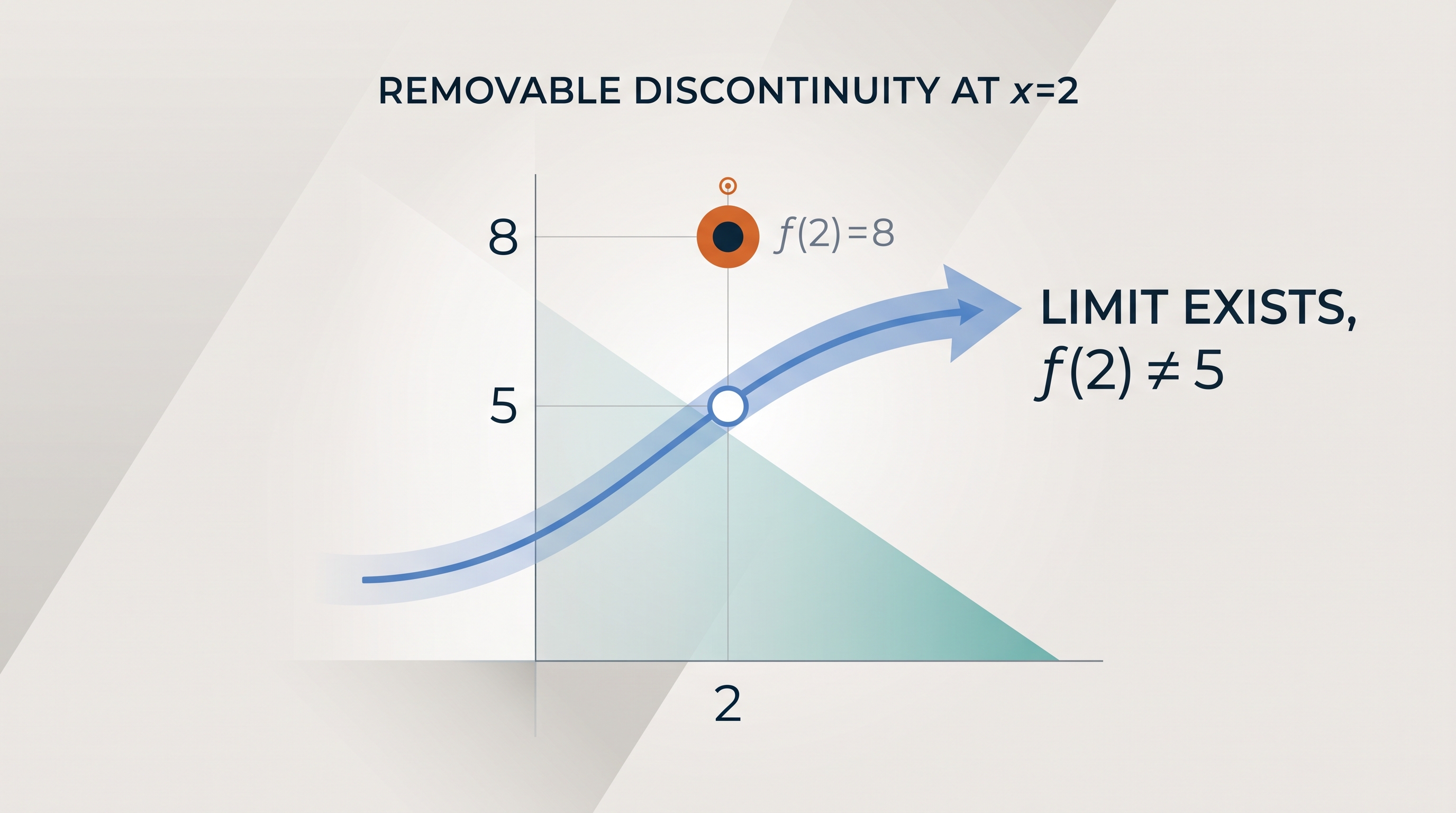
A graph has a hole at $(2,5)$, and the curve approaches $5$ from both sides. A filled point appears at $(2,8)$. State $\lim_{x\to 2}f(x)$, $f(2)$, and the type of discontinuity.
The answers are
$$ \lim_{x\to 2}f(x)=5,\qquad f(2)=8, $$
and the discontinuity is removable. The limit follows the approaching curve; the function value follows the filled point.
1.11 Defining Continuity at a Point
Key concepts: Defining continuity at a point · Using correct continuity notation and justification
The three-condition definition of continuity at a point, and how to justify a discontinuity by naming the condition that fails.
1.11 Defining Continuity at a Point
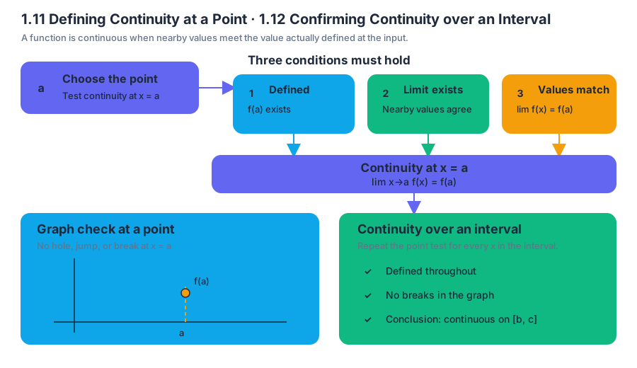
A function is continuous at $x=a$ when its graph has no break at that input: the function is defined there, its nearby values approach a single limit, and that limit equals the actual function value.
The three-condition test at a point
The formal test is not merely “the graph looks connected.” To justify continuity at $x=a$, verify all three conditions:
A function $f$ is continuous at $x=a$ if and only if
$1.$ $f(a)$ is defined;
$2.$ $\displaystyle\lim_{x\to a}f(x)$ exists; and
$3.$ $\displaystyle\lim_{x\to a}f(x)=f(a)$.
If even one condition fails, $f$ is discontinuous at $x=a$. The strongest AP-style justification identifies the failed condition rather than simply stating that the function is “not smooth” or that its graph “has a hole.”
Worked example: a temperature sensor with a missing reading
Suppose a sensor model is
$$ T(t)=\frac{t^2-9}{t-3}, $$
where $t$ is time in minutes. At $t=3$,
$$ T(3)=\frac{3^2-9}{3-3}=\frac{0}{0}, $$
so $T(3)$ is not defined. Although algebraic simplification gives
$$ T(t)=t+3 \qquad (t\ne 3), $$
the original function still has no value at $t=3$. Therefore, $T$ is not continuous at $t=3$ because Condition 1 fails. The simplified expression describes the nearby behavior, but it does not automatically create the missing value.
Misconception check — “The limit equals the formula after cancellation, so the function is continuous.” Cancellation can reveal the limit, but continuity also requires an actual function value at the point. Always check $f(a)$ separately.
Reasoning and retrieval check
Each condition can fail on its own. In the sensor example Condition 1 failed. At a jump, where the left- and right-hand limits differ, Condition 2 fails. When the limit exists and $f(a)$ is defined but the two numbers differ—a hole with a filled point at another height—Condition 3 fails. A strong justification states $f(a)$ and $\lim_{x\to a}f(x)$ explicitly and names the condition that decides the question.
Retrieval check: Let $f(x)=x+1$ for $x\ne2$ and $f(2)=5$. Is $f$ continuous at $x=2$? Here $f(2)=5$ is defined and $\lim_{x\to2}f(x)=3$ exists, but $3\ne5$, so Condition 3 fails and $f$ is discontinuous at $x=2$.
1.12 Confirming Continuity over an Interval
Key concepts: Confirming continuity over an interval · A function is continuous on an interval when it is continuous at every point in that interval · Checking continuity on closed intervals · Checking continuity on open intervals · Checking continuity on half-open intervals · Identifying functions that are not continuous at an interval point · Using correct continuity notation and justification
How to confirm continuity on open, closed and half-open intervals using the domains of standard functions and one-sided limits at included endpoints.
1.12 Confirming Continuity over an Interval
Topic 1.11 defined continuity at a single point: $f(a)$ is defined, $\lim_{x\to a}f(x)$ exists, and the two are equal. Most results in calculus, such as the Intermediate Value Theorem, need more than that—continuity on a whole interval. This page shows how to confirm it without testing infinitely many points one at a time.
Continuity on an interval
The pointwise definition scales directly to intervals:
LIM-2.B.1: A function is continuous on an interval if the function is continuous at each point in the interval.
This means that a claim such as “$f$ is continuous on $[0,4]$” is a global claim supported by pointwise reasoning. You must know that every point from $0$ through $4$ passes the continuity test, including the endpoints under the appropriate one-sided interpretation.
A powerful shortcut is supplied by LIM-2.B.2:
LIM-2.B.2: Polynomial, rational, power, exponential, logarithmic, and trigonometric functions are continuous on all points in their domains.
For example, $p(x)=x^4-2x+7$ is continuous everywhere because it is a polynomial. The rational function
$$ r(x)=\frac{x+1}{x-2} $$
is continuous wherever it is defined, so it is continuous on $[0,1]$, but not continuous on $[0,3]$ because $x=2$ lies in that interval and makes the denominator zero.
Interval endpoints: closed, open, and half-open
At an interior point, continuity uses the two-sided limit. At an endpoint, only values from inside the interval matter.
| Interval | Points to check | Endpoint interpretation |
|---|---|---|
| $[a,b]$ | Every interior point plus $a$ and $b$ | Use $\displaystyle\lim_{x\to a^+}f(x)=f(a)$ and $\displaystyle\lim_{x\to b^-}f(x)=f(b)$ |
| $(a,b)$ | Every point strictly between $a$ and $b$ | No endpoint values are included |
| $[a,b)$ | Every point from $a$ through, but not including, $b$ | Check $a$ from the right; do not check $b$ as a point in the interval |
| $(a,b]$ | Every point after $a$ through $b$ | Do not check $a$; check $b$ from the left |
Worked example: one function, three interval claims
Consider
$$ g(x)=\ln(x+2). $$
Its domain is $x>-2$. Because logarithmic functions are continuous on all points in their domains by LIM-2.B.2, $g$ is continuous on $[0,5]$, $(0,5)$, and $[0,5)$. At the included endpoint $x=0$, the relevant statement is
$$ \lim_{x\to 0^+}\ln(x+2)=\ln 2=g(0). $$
The endpoint $x=5$ requires no check for $[0,5)$ because $5$ is not part of that interval.
Now consider
$$ h(x)=\frac{1}{x+1}. $$
It is continuous on $[-2,0]$ only if its domain contains every point in that interval. But $x=-1$ lies in $[-2,0]$, and $h(-1)$ is undefined. Thus $h$ is not continuous on $[-2,0]$. It is continuous on $[-2,-1)$ and on $(-1,0]$, because the excluded point is not part of either interval.
Misconception check — “Endpoints always require two-sided limits.” For continuity on $[a,b]$, the endpoint $a$ is tested from the right and $b$ from the left. A two-sided limit would ask about values outside the interval, which are irrelevant to continuity over that interval.
AP reasoning: claim, evidence, conclusion
The relevant AP practices are Implementing Mathematical Processes, Connecting Representations, Justification, and Communication and Notation. In practice, a strong response identifies the function type or problematic point, states the domain or endpoint limit being used, and concludes with the exact interval claim.
A complete justification might read: “The function $r(x)=\frac{x+1}{x-2}$ is rational and therefore continuous on its domain. Since $2\notin[0,1]$, $r$ is continuous on $[0,1]$.” That reasoning is stronger than “the graph has no breaks,” because it names the theorem and checks the interval’s domain.
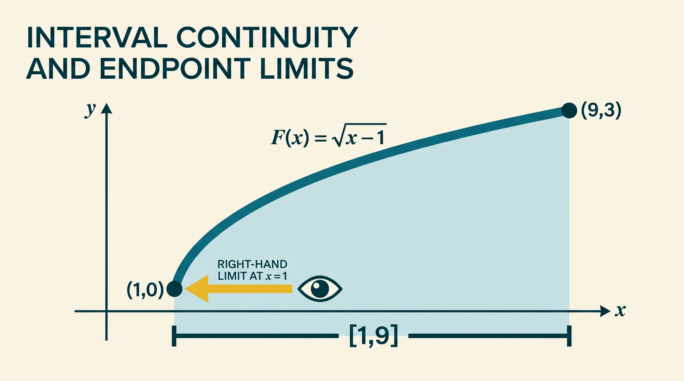
Retrieval check
For $F(x)=\sqrt{x-1}$, decide whether $F$ is continuous on $[1,9]$. What type of endpoint limit is needed at $x=1$? The answer is yes: $F$ is a power function continuous throughout its domain $[1,\infty)$, and at $x=1$ continuity is confirmed with the right-hand limit $\displaystyle\lim_{x\to1^+}F(x)=F(1)=0$.
1.13 Removing Discontinuities
Key concepts: Removing discontinuities · Removable discontinuities · Jump discontinuities · Continuity at a point · Using the definition of continuity · Applying notation for existence theorems · Solving procedures with and without technology
How to find the one value that fills a hole in a graph and makes a function continuous, and why jumps and vertical asymptotes cannot be repaired that way.
1.13 Removing Discontinuities
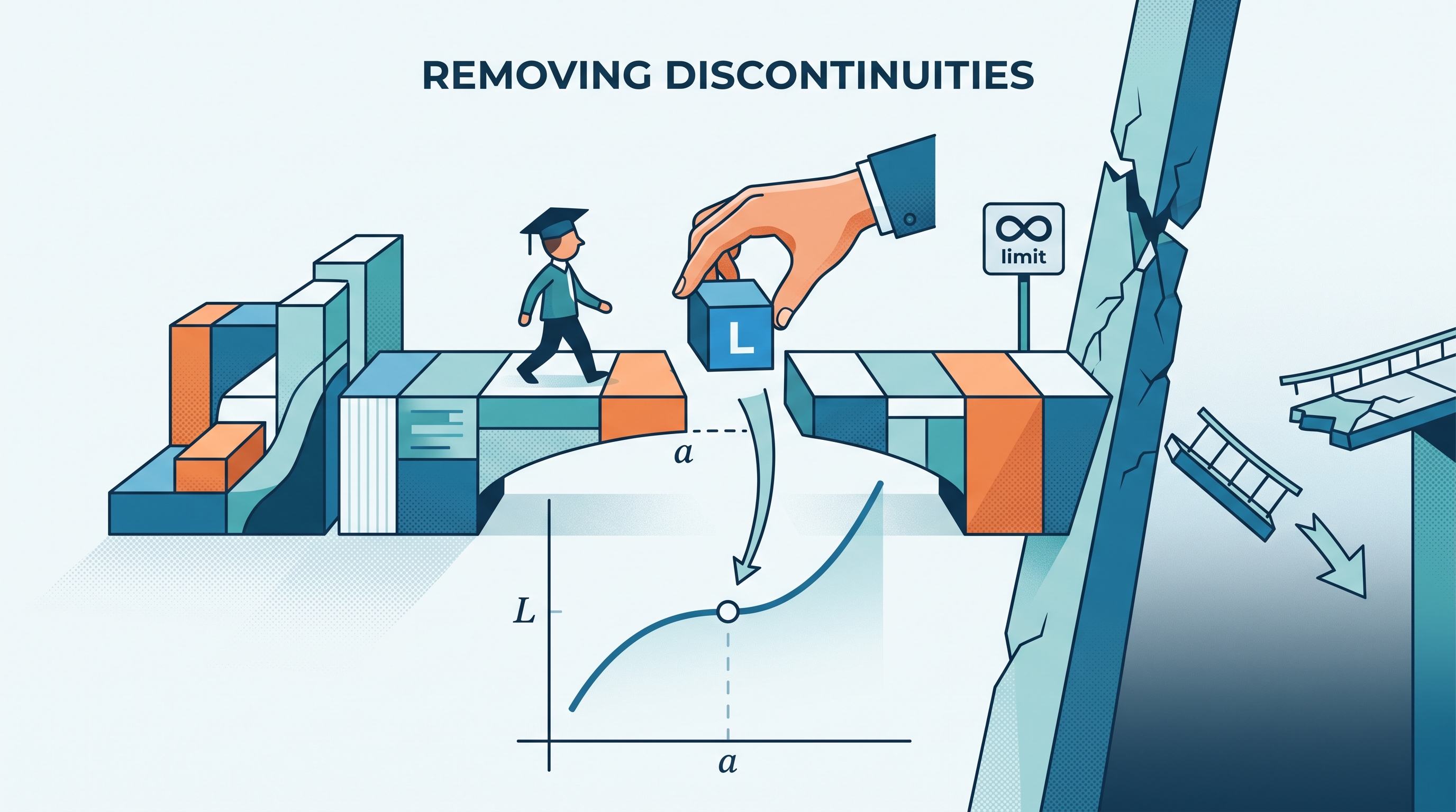
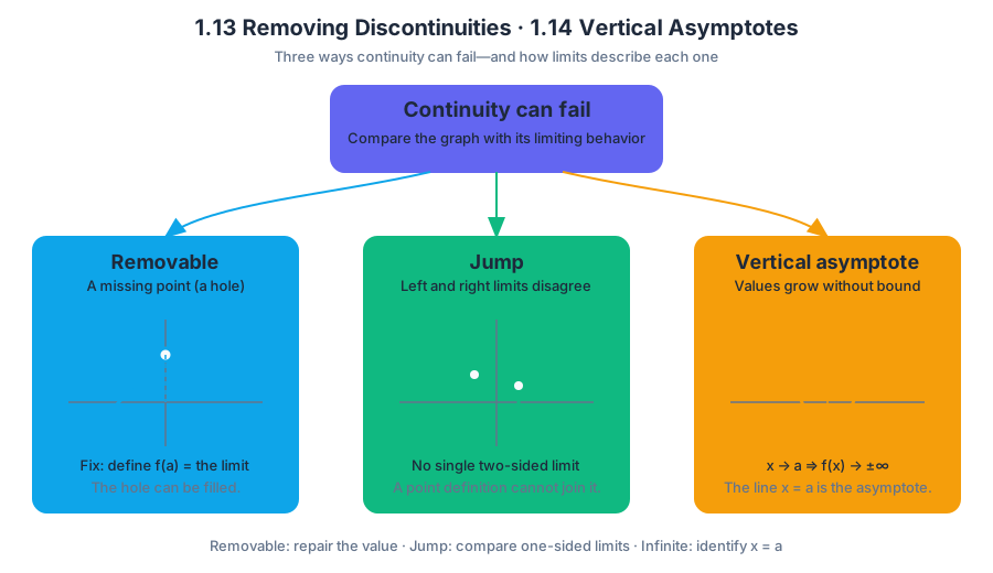
A graph can fail to be continuous in three fundamentally different ways: a missing point, a sudden jump, or an unbounded plunge toward a vertical line. These are removable discontinuities, jump discontinuities, and discontinuities due to vertical asymptotes.
Three ways continuity can fail
| Type | What the graph does near $x=a$ | Can one value of $f(a)$ repair it? |
|---|---|---|
| Removable discontinuity | Both sides approach the same finite number, but the point is missing or assigned incorrectly | Yes, by defining $f(a)$ to equal the common limit |
| Jump discontinuity | The left-hand and right-hand limits approach different finite numbers | No |
| Vertical-asymptote discontinuity | Function values increase or decrease without bound near $x=a$ | No finite value can repair it |
The previously established continuity test is the deciding tool: compare the function’s value at the point with the behavior of the function as $x$ approaches that point. For a removable discontinuity, the limiting behavior is consistent but the assigned point is not. For a jump or vertical asymptote, the surrounding behavior itself prevents continuity.
Removing a removable discontinuity
Suppose
$$ f(x)=\frac{x^2-9}{x-3}. $$
At $x=3$, direct substitution produces $\frac{0}{0}$, but factoring reveals the structure:
$$ f(x)=\frac{(x-3)(x+3)}{x-3}=x+3,\qquad x\ne 3. $$
Thus,
$$ \lim_{x\to 3}f(x)=\lim_{x\to 3}(x+3)=6. $$
The original function has a hole at $(3,6)$. It becomes continuous after defining
$$ f(3)=6. $$
This is a repair, not a change to the nearby rule: every value with $x\ne 3$ remains unchanged. Algebra removes the common factor, while the limit identifies the single value needed to fill the hole.
With and without technology
Without technology, factor, rationalize, or otherwise manipulate the expression before evaluating the limit. With technology, graph the function and use a table whose $x$-values approach $3$ from both sides. A calculator may display values close to $6$, but it cannot by itself prove that the missing point should be assigned exactly $6$; the symbolic reasoning supplies that justification.
A piecewise definition can make the repair explicit:
$$ F(x)= \begin{cases} \dfrac{x^2-9}{x-3}, & x\ne 3,\[6pt] 6, & x=3. \end{cases} $$
Then $F$ is continuous at $x=3$ because the value assigned at the point agrees with the common limiting value.
Jump discontinuities cannot be repaired
Consider
$$ g(x)= \begin{cases} x+1, & x<2,\ x+4, & x\ge 2. \end{cases} $$
The one-sided limits are
$$ \lim_{x\to 2^-}g(x)=3 \qquad\text{and}\qquad \lim_{x\to 2^+}g(x)=6. $$
Because these values differ,
$$ \lim_{x\to 2}g(x)\ \text{does not exist}. $$
Changing $g(2)$ cannot make the two sides agree. This is a jump discontinuity, often used to model an instantaneous change in a rule, price, tax bracket, or control setting.
When invoking the condition for existence of a two-sided limit, use precise notation:
$$ \lim_{x\to a}f(x)\text{ exists} \quad\Longleftrightarrow\quad \lim_{x\to a^-}f(x)=\lim_{x\to a^+}f(x), $$
provided both one-sided limits exist as the same finite value. Writing only “the limit is undefined” is weaker than identifying the unequal one-sided limits.
AP reasoning and retrieval check
This topic develops LIM-2.A and LIM-2.A.1: Justify conclusions about continuity at a point using the definition, especially by classifying the failure and deciding whether it can be repaired. It also uses 3.B: Identify an appropriate mathematical definition, theorem, or test to apply and 3.D: Apply an appropriate mathematical definition, theorem, or test. Strong responses connect a graph, equation, or table to correct one-sided-limit notation and a justified conclusion.
Retrieval check: For
$$ p(x)=\frac{x^2-16}{x-4}, $$
identify the discontinuity at $x=4$, determine whether it is removable, and state the value that repairs it. Then compare with
$$ q(x)=\frac{1}{x-4}. $$
The first function has a removable discontinuity because its simplified rule is $x+4$ and the missing value is $8$. The second has a vertical asymptote at $x=4$ because its one-sided values are unbounded; it cannot be repaired by assigning a finite value.
1.14 Connecting Infinite Limits and Vertical Asymptotes
Key concepts: Connecting infinite limits and vertical asymptotes · Discontinuities caused by vertical asymptotes · Continuity at a point · Using the definition of continuity
What an infinite limit means, how one-sided infinite limits identify a vertical asymptote, and how to tell an asymptote from a removable hole.
1.14 Connecting Infinite Limits and Vertical Asymptotes
Topic 1.13 dealt with discontinuities that one well-chosen value can repair. This page covers a failure that no value can repair: near certain inputs a function's outputs grow without bound. Limit notation is extended to describe that behavior, and on the graph it appears as a vertical asymptote.
Infinite limits and vertical asymptotes
A vertical asymptote is a vertical line $x=a$ that the graph approaches while function values grow without bound. The corresponding notation is an infinite limit:
$$ \lim_{x\to a^-}f(x)=\infty, \qquad \lim_{x\to a^+}f(x)=-\infty, $$
or another appropriate one-sided combination. The symbol $\infty$ describes unbounded behavior; it is not an ordinary number that the function reaches.
For example,
$$ h(x)=\frac{1}{(x-2)^2} $$
satisfies
$$ \lim_{x\to 2^-}h(x)=\infty \qquad\text{and}\qquad \lim_{x\to 2^+}h(x)=\infty. $$
Therefore, $x=2$ is a vertical asymptote. No definition of the single value $h(2)$ can make the function continuous there, because nearby outputs are unbounded rather than approaching one finite target.
For a rational function, a zero of the denominator produces a vertical asymptote only if it survives cancellation: $\frac{x^2-9}{x-3}$ has a hole at $x=3$, while $\frac{1}{x-3}$ has an asymptote there. The sign of a one-sided infinite limit comes from the signs of the pieces. For $r(x)=\frac{x+2}{x-5}$, the numerator is near $7$, and the denominator is small and negative just left of $5$ but small and positive just right of $5$. So $\lim_{x\to5^-}r(x)=-\infty$ and $\lim_{x\to5^+}r(x)=\infty$, and either statement justifies the asymptote $x=5$.
Misconception check — “A vertical asymptote means the limit equals infinity.” More precisely, an infinite limit means that function values exceed every bound as $x$ approaches the input value from the specified side. Since $\infty$ is not a real output, the two-sided limit is not a finite limit even when both sides tend toward $\infty$.
Hole or asymptote?
Retrieval check: For
$$ p(x)=\frac{x^2-16}{x-4}, $$
identify the discontinuity at $x=4$, determine whether it is removable, and state the value that repairs it. Then compare with
$$ q(x)=\frac{1}{x-4}. $$
The first function has a removable discontinuity because its simplified rule is $x+4$ and the missing value is $8$. The second has a vertical asymptote at $x=4$ because its one-sided values are unbounded; it cannot be repaired by assigning a finite value.
1.15 Connecting Limits at Infinity and Horizontal Asymptotes
Key concepts: Limits at infinity · Horizontal asymptotes · Limits and continuity · Graphical, numerical, analytical, and verbal representations · Geometric series · Finite sums of infinite geometric series
What limits at infinity say about end behavior, how they produce horizontal asymptotes, and how to evaluate them for rational functions and compare growth rates.
1.15 Connecting Limits at Infinity and Horizontal Asymptotes
A function can keep changing forever while its output settles toward a fixed value. That “destination” is described by a limit at infinity, and the corresponding graph feature is a horizontal asymptote.
Limits at infinity and end behavior
The statement
$$ \lim_{x\to\infty}f(x)=L $$
means that $f(x)$ approaches $L$ as $x$ increases without bound. Similarly,
$$ \lim_{x\to-\infty}f(x)=L $$
describes what happens as $x$ decreases without bound. These are statements about end behavior, not about the value of the function at any finite input.
Horizontal asymptote: The line $y=L$ is a horizontal asymptote of $f$ if $\lim_{x\to\infty}f(x)=L$ or $\lim_{x\to-\infty}f(x)=L$.
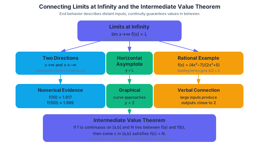
For example, consider
$$ f(x)=\frac{4x^2-7}{2x^2+5}. $$
Divide numerator and denominator by $x^2$:
$$ f(x)=\frac{4-\frac{7}{x^2}}{2+\frac{5}{x^2}}. $$
As $x\to\infty$ or $x\to-\infty$, both $\frac{7}{x^2}$ and $\frac{5}{x^2}$ approach $0$, so
$$ \lim_{x\to\pm\infty}f(x)=\frac{4}{2}=2. $$
Therefore, $y=2$ is a horizontal asymptote.
The same conclusion appears in several representations:
- Analytical: the highest-degree terms give $\frac{4x^2}{2x^2}=2$.
- Numerical: $f(10)=\frac{393}{205}\approx1.917$, while $f(100)\approx1.999$.
- Graphical: the curve approaches the line $y=2$ at both ends.
- Verbal: for very large positive or negative inputs, the output becomes close to $2$.
This is the suggested skill 2.D Connecting Representations: Identify how mathematical characteristics or properties of functions are related in different representations.
The essential knowledge for Topic 1.15 is LIM-2.D.3, which extends limits to infinity; LIM-2.D.4, which connects limits at infinity with end behavior; and LIM-2.D.5, which uses limits to compare relative magnitudes and rates of change. For instance,
$$ \lim_{x\to\infty}\frac{x^2}{e^x}=0 $$
shows analytically that exponential growth eventually dominates quadratic growth. The graph and a sufficiently far-right table should show the ratio approaching $0$ as well.
A related limit appears when adding a finite number of terms from a geometric pattern. If
$$ S_n=1+r+r^2+\cdots+r^{n-1} =\frac{1-r^n}{1-r}, $$
then for $|r|<1$, the term $r^n$ approaches $0$ as $n\to\infty$. Thus,
$$ \lim_{n\to\infty}S_n=\frac{1}{1-r}. $$
The limit describes the eventual value approached by the finite sums; it is not obtained by simply substituting infinity into the formula.
Retrieval check: Find $\lim_{x\to\infty}\frac{5x+1}{x^2+4}$ and name the horizontal asymptote. Dividing every term by $x^2$ gives $\frac{5/x+1/x^2}{1+4/x^2}$, which approaches $\frac{0}{1}=0$. The asymptote is $y=0$: the denominator's higher degree makes it grow faster than the numerator.
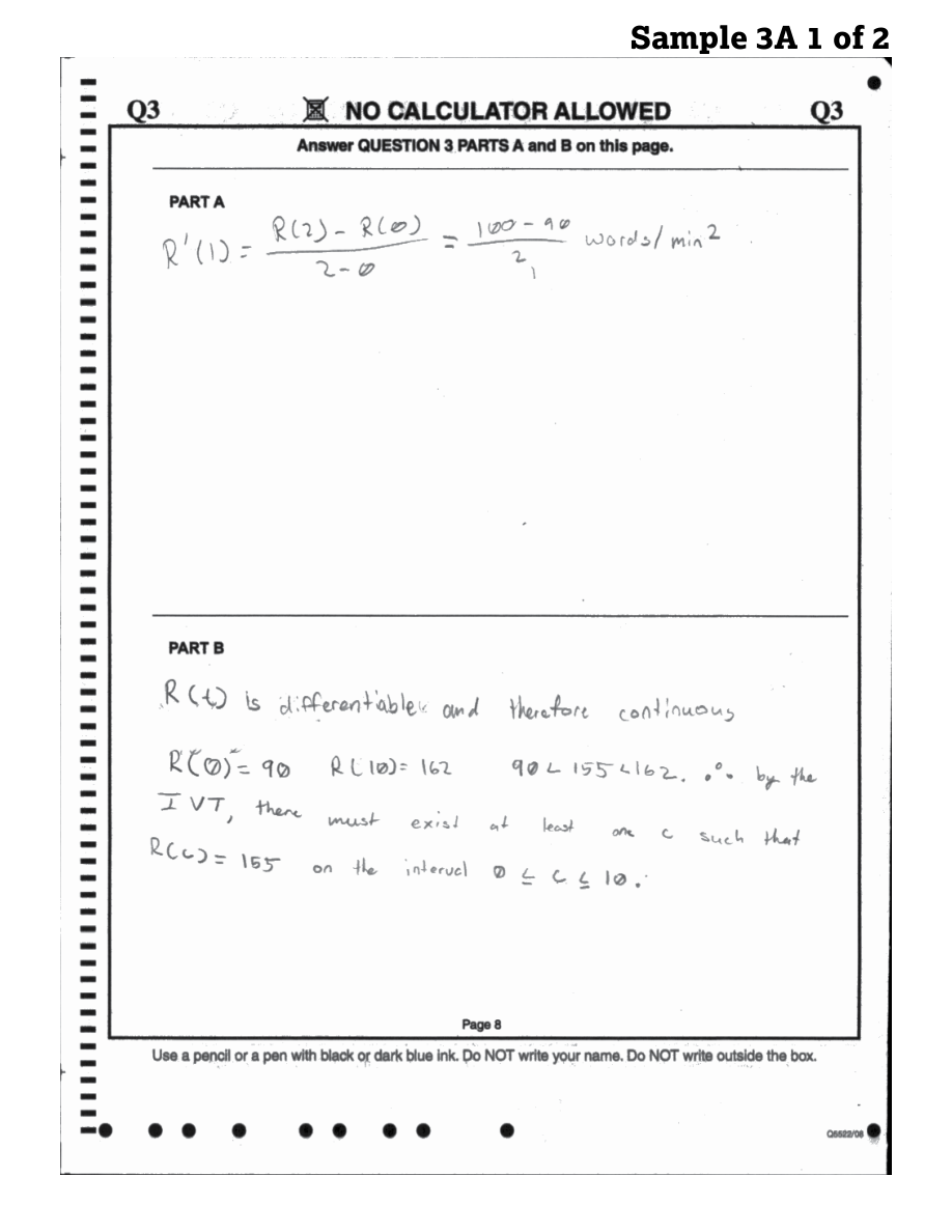
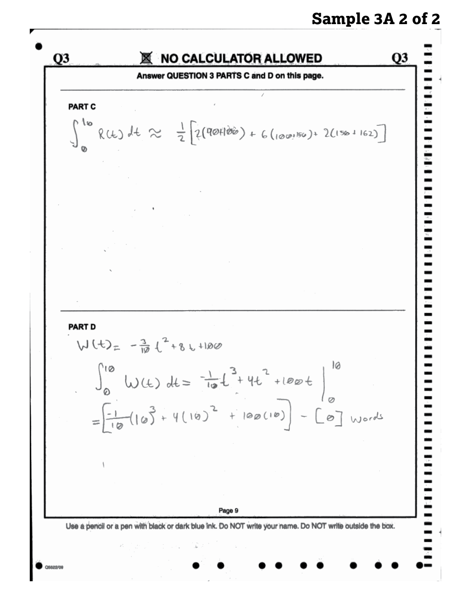
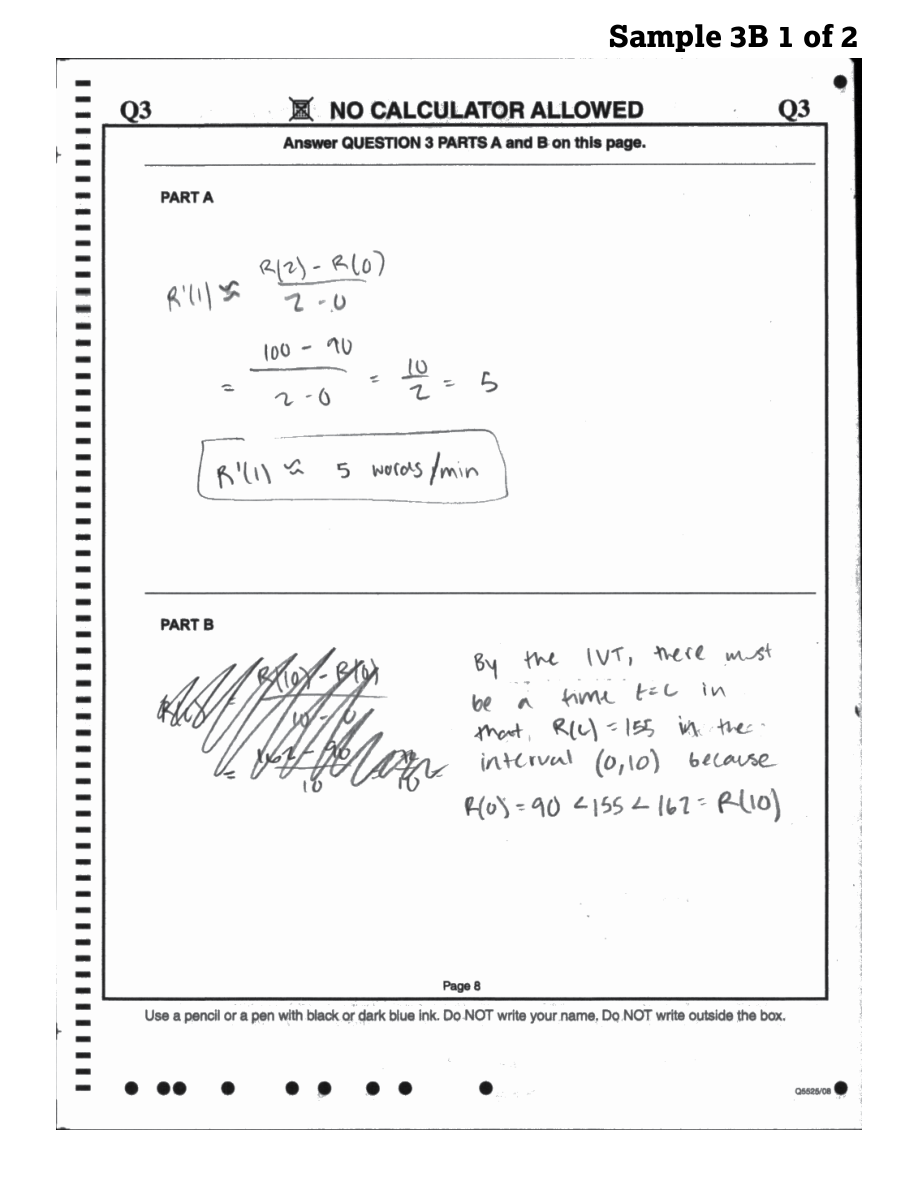
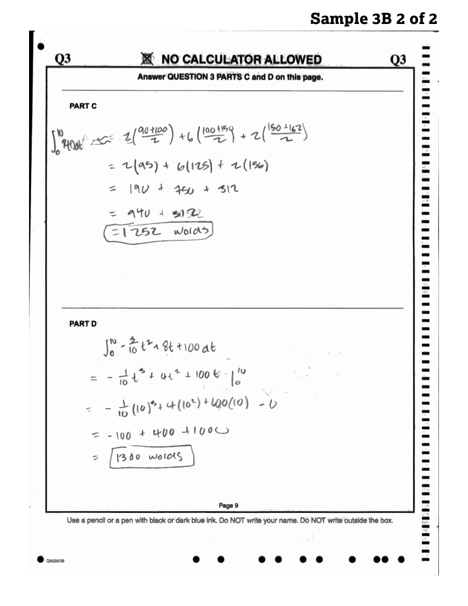
1.16 Working with the Intermediate Value Theorem
Key concepts: Intermediate Value Theorem (IVT) · Limits and continuity · Mathematical definitions, theorems, and properties · Hypotheses of theorems · Continuity of piecewise functions
The Intermediate Value Theorem: its two hypotheses, how to use it to guarantee a solution in an interval, and how to check continuity at a piecewise boundary first.
1.16 Working with the Intermediate Value Theorem
The Intermediate Value Theorem turns continuity into a guarantee: a continuous function cannot get from one output to another without taking every value in between. Because the theorem applies only when a function is continuous on an entire closed interval, this page first checks continuity where it most often fails—at the boundary of a piecewise rule—and then states and applies the theorem.
Continuity at a piecewise boundary
At a boundary point of a piecewise function, evaluating the function and finding the approaching value are separate jobs. For continuity at $x=a$, all three must agree:
$$ \lim_{x\to a^-}f(x)=\lim_{x\to a^+}f(x)=f(a). $$
A graph may approach one height while the function is assigned a different height—or no value at all.
For
$$ g(x)= \begin{cases} x+3, & x<2,\ kx-1, & x\ge 2, \end{cases} $$
continuity at $x=2$ requires the left-hand limit, right-hand limit, and defined value to match. The left side approaches
$$ \lim_{x\to2^-}(x+3)=5. $$
The right-hand value is
$$ g(2)=2k-1, $$
so continuity requires
$$ 2k-1=5, \qquad k=3. $$
This uses 2.B Connecting Representations: Identify mathematical information from graphical, numerical, analytical, and/or verbal representations.
Misconception check — “The limit is the function value.”
A limit describes what outputs approach; $f(a)$ is the output actually assigned at $a$. They are equal only when the continuity condition holds.
The Intermediate Value Theorem
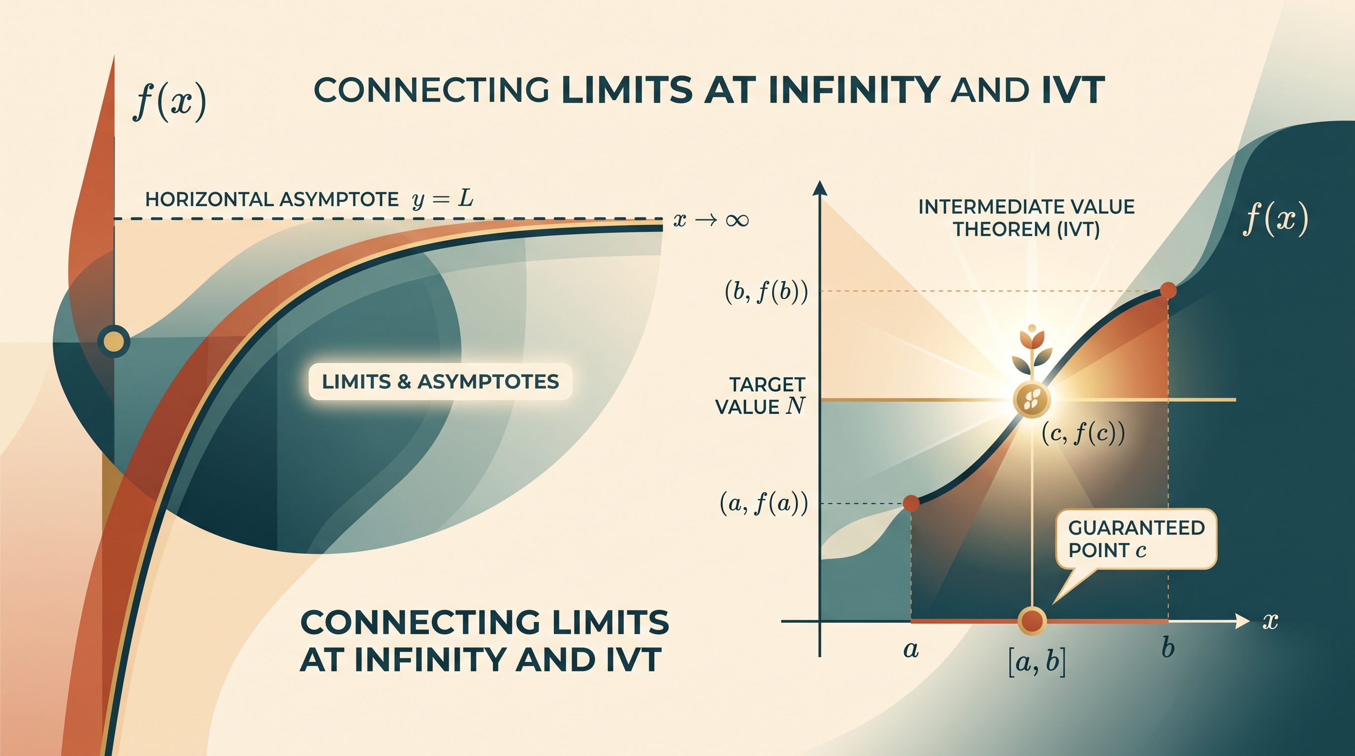
The Intermediate Value Theorem (IVT) guarantees that a continuous function cannot jump over a value. If $f$ is continuous on the closed interval $[a,b]$ and $N$ lies between $f(a)$ and $f(b)$, then there is at least one number $c$ in $(a,b)$ such that
$$ f(c)=N. $$
The hypotheses matter:
- $f$ must be continuous on every point of $[a,b]$.
- The target value $N$ must lie between the endpoint values.
Suppose
$$ h(x)=x^3-4x+1. $$
Because polynomials are continuous everywhere, $h$ is continuous on $[0,2]$. Also,
$$ h(0)=1 \quad\text{and}\quad h(2)=1. $$
These endpoints do not trap the value $0$, so the IVT cannot establish a zero on $[0,2]$. On $[-1,0]$,
$$ h(-1)=4,\qquad h(0)=1, $$
so that interval still does not trap $0$. But on $[0,1]$,
$$ h(0)=1,\qquad h(1)=-2. $$
Since $0$ lies between $1$ and $-2$, the IVT guarantees some $c\in(0,1)$ with $h(c)=0$.
If continuity fails, the conclusion can fail. A function with a jump may have endpoint values on opposite sides of $N$ but never equal $N$ inside the interval. Likewise, if $N$ is outside the endpoint range, continuity cannot force the function to reach it.
Justification pattern: State continuity on $[a,b]$, state the endpoint values, identify the trapped target value, and conclude that a point $c\in(a,b)$ exists.
Retrieval check: If $\lim_{x\to\infty}f(x)=4$, what horizontal asymptote follows? For the IVT, is “$f$ is continuous at $a$ and $b$” enough, or must continuity hold on the entire interval $[a,b]$? The answers are $y=4$ and continuity on the entire interval is required.
2.1 Defining Average and Instantaneous Rates of Change at a Point
Key concepts: Average rate of change over an interval · Instantaneous rate of change at a point · Defining the derivative using a limit · Modeling dynamic change · The relationship between average rates of change and instantaneous rates of change · Limits as foundational tools for understanding derivatives · Continuity and its connection to limits
How the average rate of change over an interval (a secant slope) becomes the instantaneous rate at a single point (a tangent slope) by taking a limit of difference quotients.
2.1 Defining Average and Instantaneous Rates of Change at a Point
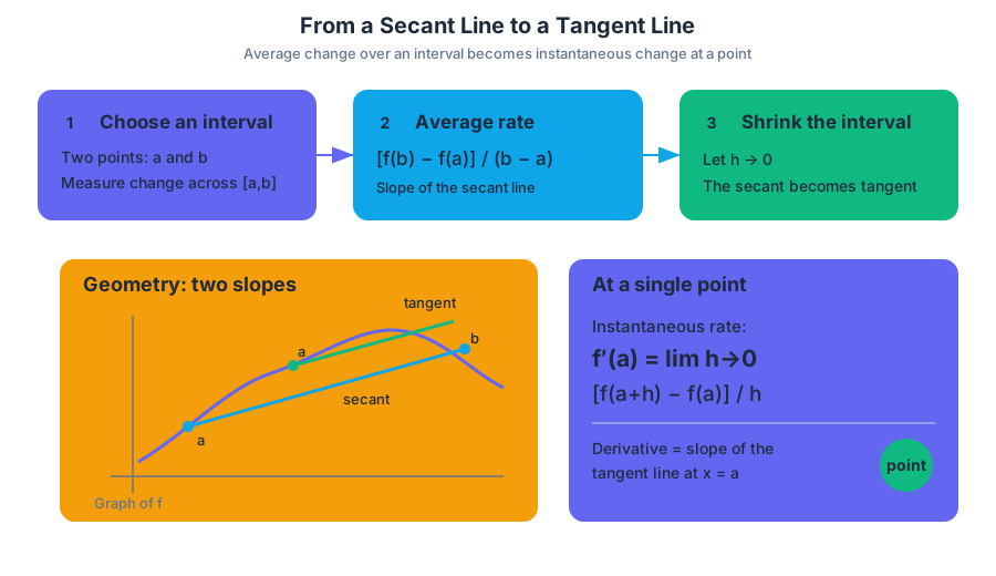
A car can travel $60$ miles in one hour, but that statement does not tell you its speed at exactly $t=23$ minutes. Average rate of change describes what happens across an interval; instantaneous rate of change describes what happens at one input value. Calculus connects them by shrinking the interval until its width approaches zero.
From a secant line to a tangent line
For a function $f$, the average rate of change over the closed interval $[a,b]$ is
$$ \frac{f(b)-f(a)}{b-a}. $$
Geometrically, this is the slope of the secant line, the line joining the two points $(a,f(a))$ and $(b,f(b))$ on the graph.
Suppose a runner’s position is modeled by $s(t)=t^2+2t$, where $s$ is measured in meters and $t$ in seconds. Over $[1,3]$,
$$ \frac{s(3)-s(1)}{3-1}
\frac{(3^2+2\cdot3)-(1^2+2\cdot1)}{2}
\frac{15-3}{2}
$$
The runner’s average velocity is therefore $6\ \text{m/s}$ during that two-second interval.
To estimate the runner’s velocity at exactly $t=1$, use an interval whose other endpoint approaches $1$. With $h$ representing the interval width, the average rate from $t=a$ to $t=a+h$ is
$$ \frac{f(a+h)-f(a)}{h}. $$
As $h\to0$, the secant line approaches the tangent line, the line that captures the graph’s direction at a single point. Its slope is the instantaneous rate of change.
The derivative at a point
The derivative at a point is the limit of average rates of change as the interval shrinks to zero. At $x=a$,
$$ f'(a)=\lim_{h\to0}\frac{f(a+h)-f(a)}{h}, $$
provided this limit exists. An equivalent form is
$$ f'(a)=\lim_{x\to a}\frac{f(x)-f(a)}{x-a}, $$
also provided the limit exists.
Key idea: A derivative is not an average over a tiny interval. It is the limiting value of those averages.
For $s(t)=t^2+2t$, find the instantaneous velocity at $t=1$:
$$ s'(1)=\lim_{h\to0}\frac{s(1+h)-s(1)}{h}. $$
Compute the numerator:
$$ s(1+h)=(1+h)^2+2(1+h)=3+4h+h^2, $$
so
$$ \frac{s(1+h)-s(1)}{h}
\frac{(3+4h+h^2)-3}{h}
4+h. $$
Therefore,
$$ s'(1)=\lim_{h\to0}(4+h)=4. $$
The runner’s instantaneous velocity at $t=1$ is $4\ \text{m/s}$. Notice that substituting $h=0$ into the original difference quotient would produce $0/0$; the algebraic simplification must occur before evaluating the limit.
AP skills and reasoning processes
Topic 2.1 develops Skill 2.B: Identify mathematical information from graphical, numerical, analytical, and/or verbal representations. A response might read a graph to identify a secant slope, use a table to form a difference quotient, or attach correct units to a rate.
Retrieval check
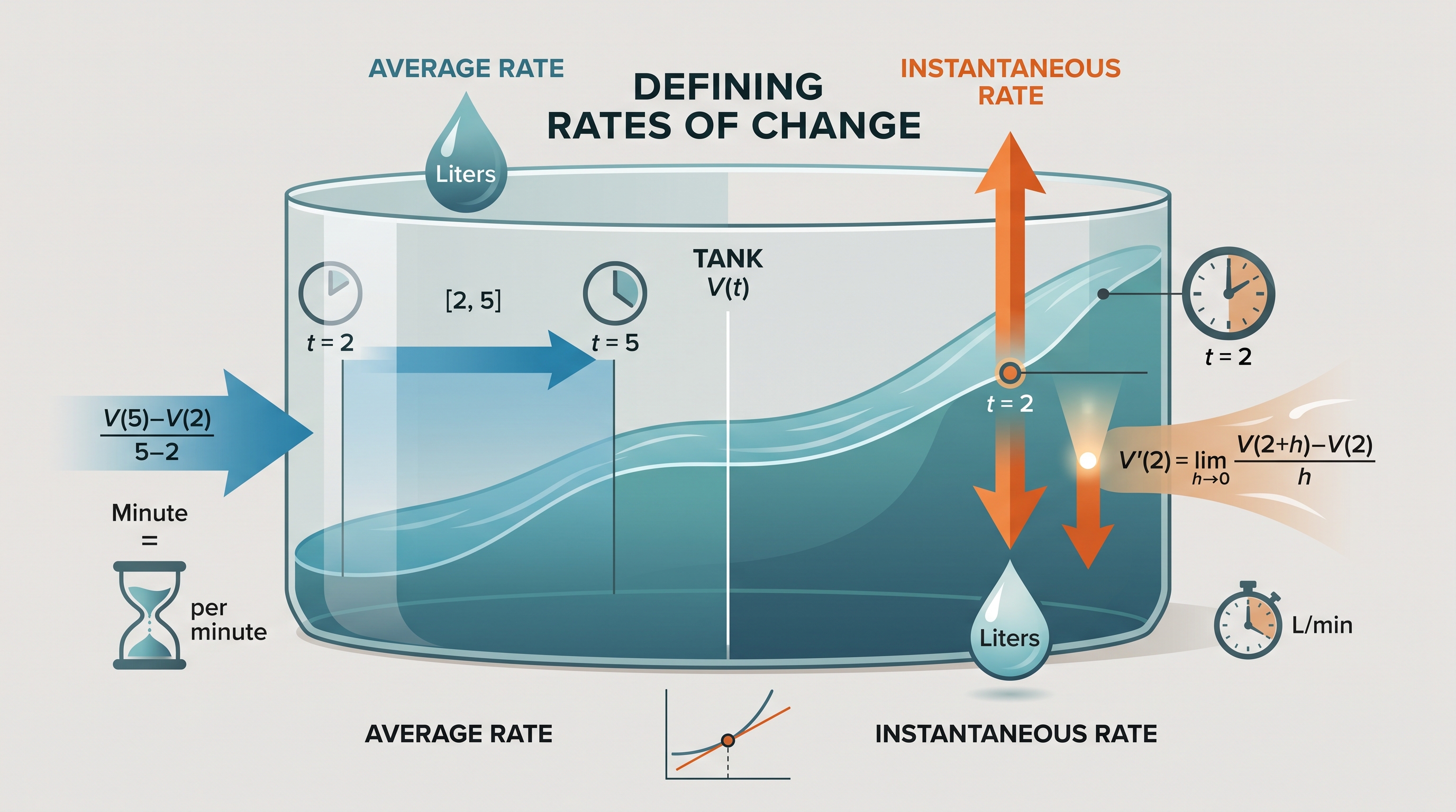
A tank contains $V(t)$ liters after $t$ minutes. Write the average rate of change on $[2,5]$, then the instantaneous rate at $t=2$ using the limit definition. What units should each rate have?
$$ \frac{V(5)-V(2)}{5-2}, \qquad V'(2)=\lim_{h\to0}\frac{V(2+h)-V(2)}{h}. $$
Both rates have units of liters per minute, but the first describes an interval and the second describes one instant.
2.2 Defining the Derivative of a Function and Using Derivative Notation
Key concepts: The derivative of a function · Defining the derivative using a limit · Derivative notation, including f'(x), y', and f' · Using analytical, numerical, graphical, and verbal representations of derivatives · Limits as foundational tools for understanding derivatives
Defines the derivative as a limit of difference quotients, treats it as a function in its own right, and explains derivative notation and the four ways a derivative is represented.
2.2 Defining the Derivative of a Function and Using Derivative Notation
Topic 2.1 found the instantaneous rate of change at a single input as a limit of average rates. This page names that limit the derivative, extends it from one input to a whole function, and sets out its notation.
The derivative at a point
The derivative at a point is the limit of average rates of change as the interval shrinks to zero. At $x=a$,
$$ f'(a)=\lim_{h\to0}\frac{f(a+h)-f(a)}{h}, $$
provided this limit exists. An equivalent form is
$$ f'(a)=\lim_{x\to a}\frac{f(x)-f(a)}{x-a}, $$
also provided the limit exists.
Key idea: A derivative is not an average over a tiny interval. It is the limiting value of those averages.
The derivative as a function
Nothing in that limit depends on the particular input $a$. Replacing $a$ with a variable $x$ defines a new function, the derivative of $f$: $f'(x)=\lim_{h\to0}\frac{f(x+h)-f(x)}{h}$, defined wherever the limit exists. For $f(x)=x^2+2x$ the difference quotient simplifies to $2x+2+h$, so $f'(x)=2x+2$ and $f'(1)=4$.
Derivative notation and representations
The derivative of $f$ with respect to $x$ may be written in several equivalent ways:
$$ f'(x), \qquad y', \qquad f'. $$
The expression $f'(x)$ emphasizes that the derivative is itself a function: each input $x$ receives the instantaneous rate of change at that location. The notation $f'(a)$ means the particular derivative value at $x=a$.
Leibniz notation $\frac{dy}{dx}$ is a fourth way to write the derivative of $y=f(x)$, read “the derivative of $y$ with respect to $x$”. It is one symbol, not a fraction to cancel; its value at $x=a$ is written $\left.\frac{dy}{dx}\right|_{x=a}$.
A derivative communicates the same idea through four representations:
| Representation | What it tells you |
|---|---|
| Analytical | A formula such as $f'(x)=2x+2$ |
| Numerical | A limit or computed value such as $f'(1)=4$ |
| Graphical | The slope of the tangent line to $y=f(x)$ |
| Verbal | “At $t=1$, position is increasing at $4\ \text{m/s}$.” |
Because $f'(a)$ is the slope of the tangent line at $(a,f(a))$, that line has equation $y=f(a)+f'(a)(x-a)$. For $f(x)=x^2+2x$ at $x=1$ this is $y=3+4(x-1)$.
AP skills and reasoning processes
Topic 2.2 develops Skill 1.D: Identify an appropriate mathematical procedure by recognizing when the limit definition of the derivative is required, and Skill 4.C: Use appropriate mathematical notation by correctly writing expressions such as $f'(a)$, $y'$, and
$$ \lim_{h\to0}\frac{f(a+h)-f(a)}{h}. $$
Misconception check
Misconception: “The derivative is just the function divided by $x$.” The derivative measures change in the output relative to change in the input; it is built from a difference quotient. Also, a derivative need not exist: if the defining limit fails to exist, then $f'(a)$ is undefined at that point.
2.3 Estimating Derivatives of a Function at a Point
Key concepts: Estimating a derivative at a point from a graph or table · Derivative as the limit of difference quotients · Interpreting a limit as the derivative of a specific function at a specific x-value
Estimating a derivative at a point from tables and graphs using nearby secant slopes, with correct units, and recognising a limit as the derivative of a particular function at a particular input.
2.3 Estimating Derivatives of a Function at a Point
Using the difference-quotient definition, estimate or identify the limiting slope at the specified point. The key question is not merely “What is the slope?” but “Do the nearby slopes approach one common finite value?”
Estimating a derivative from a table or graph
A derivative at $x=a$ can be estimated from nearby secant slopes, which measure average change over an interval. As the interval narrows around $a$, those secant slopes approximate the tangent slope:
$$ f'(a)=\lim_{h\to 0}\frac{f(a+h)-f(a)}{h}, $$
when the limit exists.
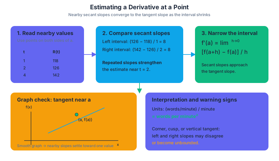
Suppose $R(t)$ gives the number of words per minute read by a student. Nearby measurements are:
| $t$ (minutes) | $R(t)$ (words per minute) |
|---|---|
| $1$ | $118$ |
| $2$ | $126$ |
| $4$ | $142$ |
To estimate $R'(2)$, use values on either side of $t=2$. From $t=1$ to $t=2$,
$$ \frac{R(2)-R(1)}{2-1} =\frac{126-118}{1}=8. $$
From $t=2$ to $t=4$,
$$ \frac{R(4)-R(2)}{4-2} =\frac{142-126}{2}=8. $$
Thus $R'(2)\approx 8$ words per minute per minute. The repeated value strengthens the estimate: the reading rate is increasing at approximately $8$ words per minute each minute at $t=2$.
The units matter. Since $R$ is measured in words per minute and $t$ in minutes, $R'(2)$ has units
$$ \frac{\text{words per minute}}{\text{minute}} =\text{words per minute}^2. $$
On a graph, estimate $f'(a)$ by inspecting the tangent line near $(a,f(a))$. If the graph has a smooth, increasingly flat shape, nearby secant slopes should settle toward one number. If the graph has a corner, cusp, or vertical tangent, the left- and right-hand slopes may fail to agree or may become unbounded.
Technology offers a third route. When a formula is available on a calculator-active question, the calculator’s numerical derivative at $x=a$ is an accepted way to obtain $f'(a)$; it works by evaluating a very narrow difference quotient.
Recognizing a derivative inside a limit
A limit with a denominator approaching $0$ often hides the difference quotient for a particular function. To identify it, match the expression to
$$ \lim_{h\to0}\frac{f(a+h)-f(a)}{h}. $$
Read the numerator as “function value near $a$ minus function value at $a$.”
For example,
$$ \lim_{h\to0}\frac{(3+h)^2-9}{h} $$
is the derivative of $f(x)=x^2$ at $x=3$, because
$$ f(3+h)=(3+h)^2 \qquad\text{and}\qquad f(3)=3^2=9. $$
Therefore,
$$ \lim_{h\to0}\frac{(3+h)^2-9}{h}=f'(3). $$
The important response is not only the numerical value; it is the mathematical identification: this limit represents the instantaneous rate of change of $f(x)=x^2$ at $x=3$.
A shifted form may require more careful reading. In
$$ \lim_{x\to 2}\frac{\sqrt{x+7}-3}{x-2}, $$
the function is $f(x)=\sqrt{x+7}$, the approached point is $a=2$, and $f(2)=\sqrt{9}=3$. Hence the limit is $f'(2)$.
Retrieval check: A table gives $f(2.9)=8.41$, $f(3)=9$ and $f(3.1)=9.61$. Compute the secant slope on each side of $x=3$ and estimate $f'(3)$. Then decide which function and point $\lim_{h\to0}\frac{(3+h)^2-9}{h}$ describes. The slopes $5.9$ and $6.1$ give $f'(3)\approx6$, consistent with the limit, which is $f'(3)$ for $f(x)=x^2$.
2.4 Connecting Differentiability and Continuity
Key concepts: Derivative as the limit of difference quotients · Differentiability at a point · Continuity at a point · The relationship between differentiability and continuity · Sharp corners or crossovers where one-sided slopes do not match · Vertical tangents where the derivative is undefined
Why differentiability at a point forces continuity there, why the converse fails at corners and vertical tangents, and how to justify a claim that a derivative does not exist.
2.4 Connecting Differentiability and Continuity
The derivative $f'(a)=\lim_{h\to0}\frac{f(a+h)-f(a)}{h}$ is a limit, and a limit does not have to exist. This page asks when $f'(a)$ exists and how that question is tied to continuity at $a$: differentiability guarantees continuity, but continuity alone does not guarantee a derivative.
Differentiability and continuity
A function is differentiable at a point if its derivative exists there as a finite, single value. A function is continuous at $x=a$ if it has no break at that point:
$$ \lim_{x\to a}f(x)=f(a). $$
The required relationship is one-way:
FUN-2.A.1: If a function is differentiable at a point, then it is continuous at that point.
The derivative definition explains why. If $f'(a)$ exists, then the nearby change can be written as
$$ f(a+h)-f(a)
h\left(\frac{f(a+h)-f(a)}{h}\right). $$
As $h\to0$, the first factor approaches $0$ and the second approaches the finite number $f'(a)$, so $f(a+h)-f(a)\to0$. Therefore $f(a+h)\to f(a)$, which is continuity.
The converse is false:
FUN-2.A.2: A continuous function may fail to be differentiable at a point in its domain.
Two standard failures are especially important:
- Sharp corner or crossover: For $f(x)=|x|$ at $x=0$, the left-hand difference quotient approaches $-1$, while the right-hand difference quotient approaches $1$. Since the one-sided slopes disagree, $f'(0)$ does not exist, even though $f$ is continuous at $0$.
- Vertical tangent: For $f(x)=\sqrt[3]{x}$ at $x=0$, the tangent is vertical. The slopes become unbounded, so there is no ordinary finite derivative at $0$.
A discontinuity also rules out differentiability immediately. In particular, if $a$ is not in the domain of $f$, then it cannot be in the domain of $f'$.
AP reasoning focus: 3.E Justification
Skill 3.E: Provide reasons or rationales for solutions and conclusions requires a reason, not just a label. “Not differentiable” is incomplete. A stronger conclusion names the mechanism: the one-sided slopes differ, the tangent is vertical, or the function is not continuous.
Misconception check: Continuity does not guarantee differentiability. Continuity means the graph has no break; differentiability additionally requires one well-defined finite tangent slope.
Retrieval check: The limit
$$ \lim_{h\to0}\frac{|4+h|-4}{h} $$
represents which derivative? Is the function differentiable at the approached point? Identify the function and point first, then compare the one-sided slopes.
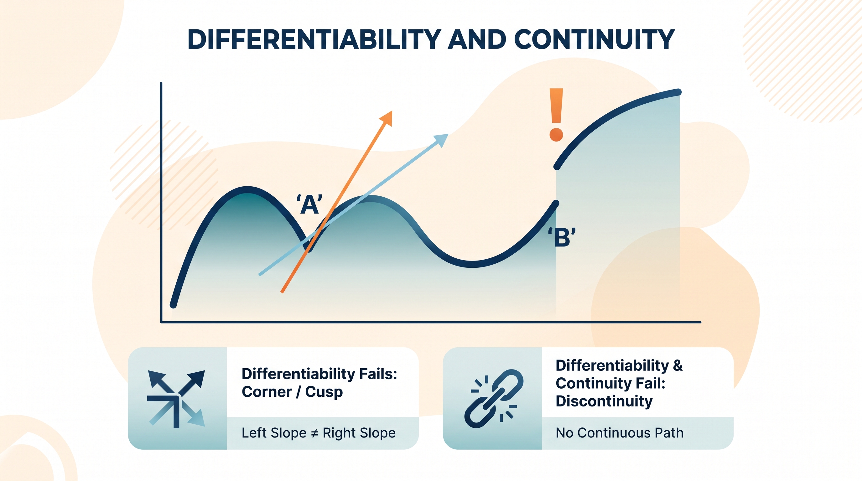
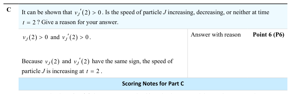
2.5 Applying the Power Rule
Key concepts: Applying the power rule · Using appropriate mathematical rules and procedures to calculate derivatives · Differentiating familiar functions · Combining the power rule with sum and difference rules
How to differentiate any power of x, including negative and fractional exponents, by bringing the exponent forward and reducing it by one, and where the rule's domain conditions matter.
2.5 Applying the Power Rule
The power rule turns the derivative of a power function into a mechanical calculation: bring the exponent forward, then reduce the exponent by $1$. Together with the constant, sum, difference, and constant multiple rules, it transforms a complicated-looking polynomial into a short list of familiar derivatives.
The power rule
For a real exponent $r$, on the domain where the expression $x^r$ is defined and differentiable,
$$ \frac{d}{dx}\left(x^r\right)=rx^{r-1}. $$
The domain qualification matters. For example, $x^{1/2}$ is real-valued only when $x\ge 0$, and its derivative formula is applied on the interior of that domain, where the function is differentiable. Likewise, negative or fractional exponents may create excluded inputs or endpoint restrictions.
A useful visual pattern is:
$$ \boxed{x^r} \quad\longrightarrow\quad \boxed{r\cdot x^{r-1}} $$
The exponent moves into the coefficient slot; the exponent itself decreases by $1$.
For a polynomial term such as $7x^5$, first apply the power rule to $x^5$, then preserve the coefficient $7$:
$$ \frac{d}{dx}(7x^5) =7\frac{d}{dx}(x^5) =7(5x^4) =35x^4. $$
For a negative exponent,
$$ \frac{d}{dx}\left(x^{-3}\right) =-3x^{-4}. $$
For a fractional exponent,
$$ \frac{d}{dx}\left(x^{1/2}\right) =\frac12x^{-1/2}. $$
The rule changes the exponent; it does not multiply the entire expression by an unrelated quantity.
Rewrite first, then differentiate
Many expressions are powers in disguise. Rewrite roots and reciprocals with exponents before differentiating: $\sqrt[3]{x}=x^{1/3}$ has derivative $\frac13x^{-2/3}$, and $\frac{1}{x^2}=x^{-2}$ has derivative $-2x^{-3}$. The simplest case follows the same pattern: $\frac{d}{dx}(x)=1\cdot x^0=1$. The rule also agrees with the limit definition: for $x^2$, the difference quotient $\frac{(x+h)^2-x^2}{h}=2x+h$ approaches $2x$.
Misconception check
Misconception: “The derivative of $7x^4$ is $4x^3$.”
The exponent rule gives the derivative of $x^4$, not of the whole term. The coefficient must remain:
$$ \frac{d}{dx}(7x^4)=7(4x^3)=28x^3. $$
Retrieval check
This check is a full polynomial. Its terms are joined by the sum, difference and constant multiple rules of Topic 2.6, but every nonconstant term is a direct use of the power rule.
Differentiate
$$ q(x)=6x^4-2x^3+5x-14. $$
Apply the power rule, sum and difference rules, constant multiple rule, and constant-function rule:
$$ \boxed{q'(x)=24x^3-6x^2+5}. $$
If a coefficient or sign changes in your answer, identify the original term that caused it before continuing.
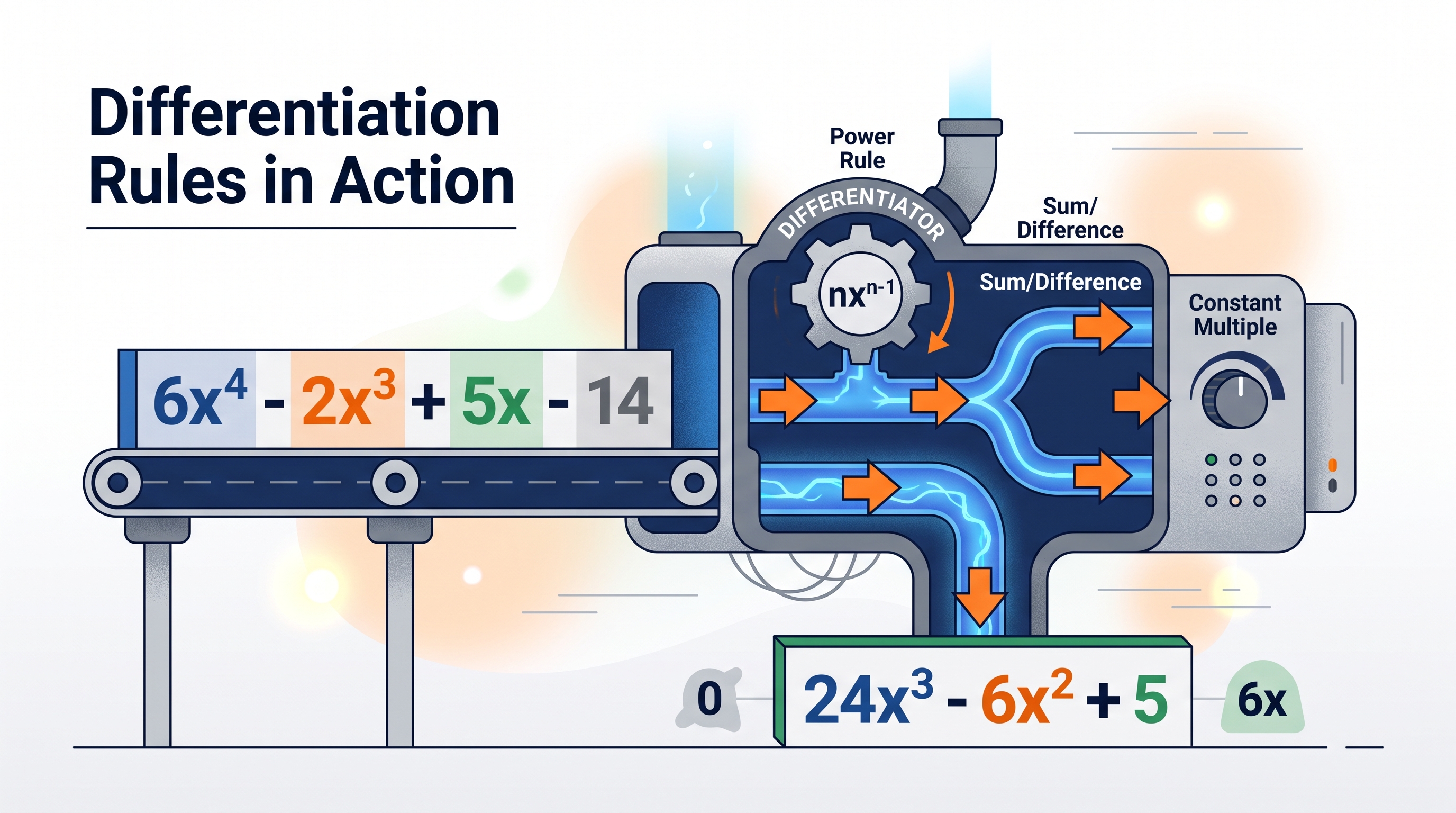
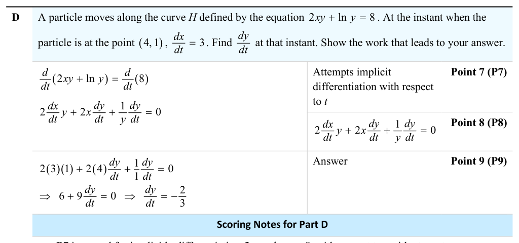
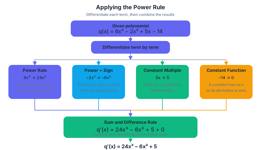
2.6 Derivative Rules: Constant, Sum, Difference, and Constant Multiple
Key concepts: Derivative rules for constant functions · Sum rule for derivatives · Difference rule for derivatives · Constant multiple rule for derivatives · Using appropriate mathematical rules and procedures to calculate derivatives · Differentiating familiar functions · Combining the power rule with sum and difference rules · Applying derivative rules with and without technology
The constant, sum, difference and constant multiple rules, why they follow from limit properties, and how they combine with the power rule to differentiate polynomials term by term.
2.6 Derivative Rules: Constant, Sum, Difference, and Constant Multiple
The power rule of Topic 2.5, $\frac{d}{dx}(x^r)=rx^{r-1}$, differentiates a single power of $x$. Most functions are built from several such pieces, scaled by coefficients, added, subtracted and shifted by constants. Four structural rules describe how a derivative passes through that algebra, so a polynomial can be differentiated one term at a time.
Learning Objective FUN-3.A: Calculate derivatives of familiar functions.
Essential Knowledge FUN-3.A.2: Sums, differences, and constant multiples of functions can be differentiated using derivative rules.
Essential Knowledge FUN-3.A.3: The power rule combined with sum, difference, and constant multiple properties can be used to find the derivatives for polynomial functions.
The four structural rules
A constant function has the same output for every input. Its graph is horizontal, so its instantaneous rate of change is zero:
$$ \frac{d}{dx}(C)=0, $$
where $C$ is any constant.
The sum rule differentiates each function separately:
$$ \frac{d}{dx}\bigl(f(x)+g(x)\bigr) =f'(x)+g'(x). $$
The difference rule works the same way:
$$ \frac{d}{dx}\bigl(f(x)-g(x)\bigr) =f'(x)-g'(x). $$
The constant multiple rule leaves a constant factor outside the derivative:
$$ \frac{d}{dx}\bigl(Cf(x)\bigr)=Cf'(x). $$
These rules are best viewed as a “preserve the structure” system:
| Function structure | Derivative action |
|---|---|
| Constant $C$ | Replace it with $0$ |
| Sum $f+g$ | Differentiate both terms and add |
| Difference $f-g$ | Differentiate both terms and subtract |
| Constant multiple $Cf$ | Keep $C$ and differentiate $f$ |
Worked example: a changing production rate
Suppose the number of components produced by a machine after $t$ hours is modeled by
$$ P(t)=4t^5-9t^3+12t-80. $$
The instantaneous production rate is $P'(t)$. Differentiate term by term:
$$ \begin{aligned} P'(t) &=\frac{d}{dt}(4t^5) -\frac{d}{dt}(9t^3) +\frac{d}{dt}(12t) -\frac{d}{dt}(80)\[4pt] &=4(5t^4)-9(3t^2)+12(1)-0\[4pt] &=20t^4-27t^2+12. \end{aligned} $$
Thus,
$$ \boxed{P'(t)=20t^4-27t^2+12}. $$
At $t=2$ hours,
$$ P'(2)=20(2^4)-27(2^2)+12 =320-108+12 =224. $$
So the model predicts an instantaneous production rate of $224$ components per hour at $t=2$.
Why term-by-term differentiation works
The derivative is built from a limit, and limits preserve sums, differences, and constant factors. That is why a polynomial does not require a new technique for every term: each term contributes its own rate of change, and those contributions combine according to the original algebraic signs and coefficients.
For instance, if
$$ f(x)=x^4-6x^2+3, $$
then
$$ f'(x)=4x^3-12x. $$
The constant $3$ contributes no change, the subtraction remains subtraction, and the coefficient $6$ remains attached to the derivative of $x^2$.
Misconception check
Misconception: “The derivative of $7x^4$ is $4x^3$.”
The exponent rule gives the derivative of $x^4$, not of the whole term. The coefficient must remain:
$$ \frac{d}{dx}(7x^4)=7(4x^3)=28x^3. $$
A second common error is differentiating a constant as though it were a variable expression:
$$ \frac{d}{dx}(11)=0, $$
not $1$ and not $11$.
A third is mishandling subtraction. The negative sign belongs to the term:
$$ \frac{d}{dx}\left(x^5-3x^2\right) =5x^4-6x, $$
not $5x^4+6x$.
Using procedures with and without technology
For a familiar polynomial, an analytical derivative is usually fastest and most informative. A graphing calculator or computer algebra system can verify the result, but technology should not replace the rule selection or the written derivative.
For
$$ h(x)=2x^3-5x+9, $$
the analytical calculation is
$$ h'(x)=6x^2-5. $$
A calculator can numerically estimate $h'(2)$, but the exact derivative immediately gives
$$ h'(2)=6(2^2)-5=19. $$
This is an instance of Suggested Skill 1.E: Apply appropriate mathematical rules or procedures, with and without technology.
Retrieval check
Differentiate
$$ q(x)=6x^4-2x^3+5x-14. $$
Apply the power rule, sum and difference rules, constant multiple rule, and constant-function rule:
$$ \boxed{q'(x)=24x^3-6x^2+5}. $$
If a coefficient or sign changes in your answer, identify the original term that caused it before continuing.
2.7 Derivatives of \(\cos x\), \(\sin x\), \(e^x\), and \(\ln x\)
Key concepts: Derivatives of cos x, sin x, e^x, and ln x · The chain rule and its applications · Maclaurin series for sin x and cos x · AP Exam assessment of derivative rules · Derivatives of tangent, cotangent, secant, and cosecant functions
The derivatives of sin x, cos x, e^x and ln x, the sign and domain conditions that go with them, and why the sine and cosine rules are consistent with their series.
2.7 Derivatives of (\cos x), (\sin x), (e^x), and (\ln x)
Polynomials are not the only functions with simple derivatives. Four more, $\sin x$, $\cos x$, $e^x$ and $\ln x$, appear in almost every later derivative because they model oscillation, growth and scaling. This page gives their derivatives and the condition attached to each.
Enduring Understanding FUN-3: Recognizing opportunities to apply derivative rules can simplify differentiation.
The essential derivative formulas
The four basic derivatives below are especially important because they recur inside products, compositions, motion models, and implicit relations.
$$ \frac{d}{dx}(\cos x)=-\sin x \qquad \frac{d}{dx}(\sin x)=\cos x $$
$$ \frac{d}{dx}(e^x)=e^x \qquad \frac{d}{dx}(\ln x)=\frac{1}{x}, \quad x>0 $$
The exponential function is remarkable because its rate of change equals its current value. The sine and cosine functions cycle into one another, with the negative sign appearing when cosine decreases. The logarithm rule requires $x>0$ because $\ln x$ is defined over the real numbers only for positive inputs.
These rules also evaluate limits that are derivatives in disguise. Because $\lim_{h\to0}\frac{\sin(\frac{\pi}{6}+h)-\frac12}{h}$ is the definition of the derivative of $\sin x$ at $x=\frac{\pi}{6}$, its value is $\cos\frac{\pi}{6}=\frac{\sqrt3}{2}$.
The chain rule inside these rules
The formulas above give derivatives of functions whose input is simply $x$. If the input is another function, use the chain rule: differentiate the outside function, keep the inside function, and multiply by the derivative of the inside.
Learning Objective FUN-3.C is to calculate derivatives of compositions of differentiable functions, supported by Essential Knowledge FUN-3.C.1: the chain rule provides a way to differentiate composite functions.
For example, with $y=\cos(3x^2)$, the outside function is cosine and the inside function is $3x^2$:
$$ \frac{dy}{dx}=-\sin(3x^2)\cdot 6x. $$
Why the trigonometric rules are trustworthy
The Maclaurin series make the sine and cosine derivatives visible term by term:
$$ \sin x=x-\frac{x^3}{3!}+\frac{x^5}{5!}-\frac{x^7}{7!}+\cdots $$
$$ \cos x=1-\frac{x^2}{2!}+\frac{x^4}{4!}-\frac{x^6}{6!}+\cdots $$
Differentiating these series produces the alternating pattern:
$$ \frac{d}{dx}(\sin x)=\cos x, \qquad \frac{d}{dx}(\cos x)=-\sin x. $$
Identities and later differentiation rules establish the remaining trigonometric derivatives without needing to memorize unrelated formulas as isolated facts.
AP assessment lens
Topic 2.7 is assessed mainly through Skill 1.E: Apply appropriate mathematical rules or procedures, with and without technology. These four derivatives rarely appear alone, so recall has to be automatic, including the negative sign in $-\sin x$ and the condition $x>0$ for $\ln x$.
On free-response work, write the derivative rule clearly, preserve factors long enough to show the structure, and include units when the quantity represents a rate. A correct final number without supporting work may not demonstrate the reasoning required by the scoring rubric.
Retrieval check: Differentiate $p(x)=4\sin x+3\cos x-2e^x+\ln x$ for $x>0$. The expected result is $p'(x)=4\cos x-3\sin x-2e^x+\frac{1}{x}$: every term keeps its coefficient, and only the cosine term changes sign.
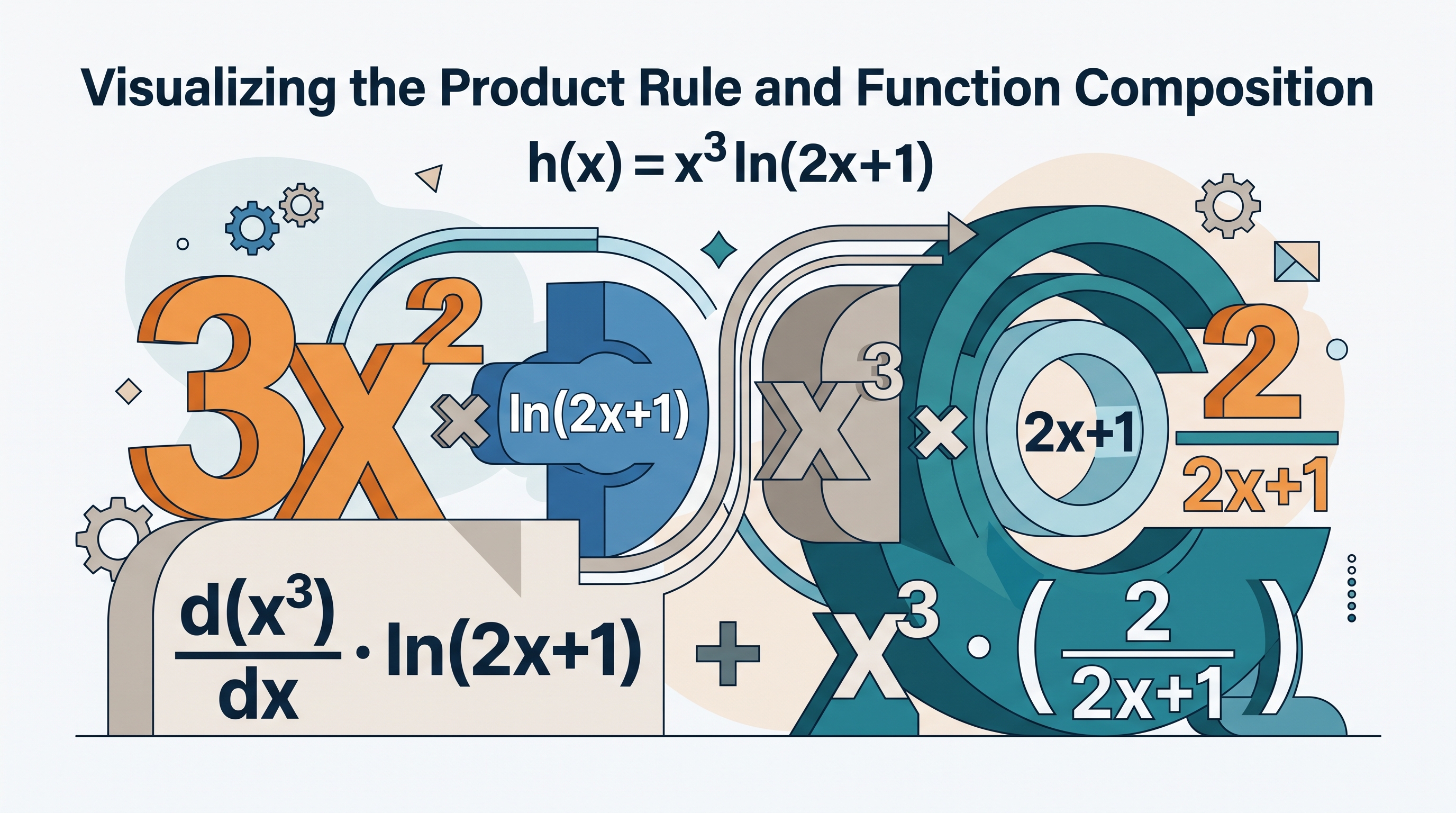
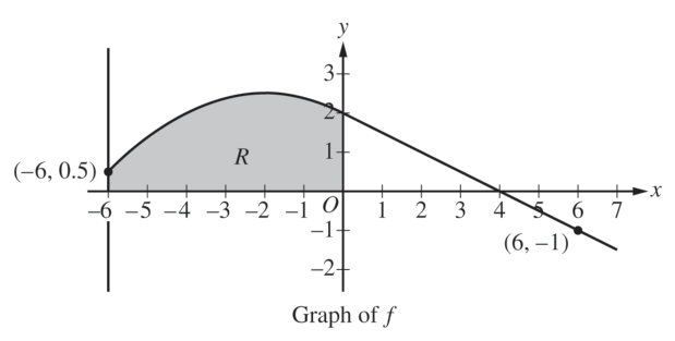
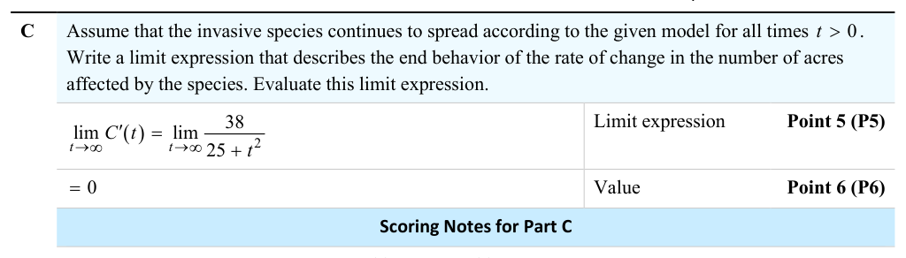
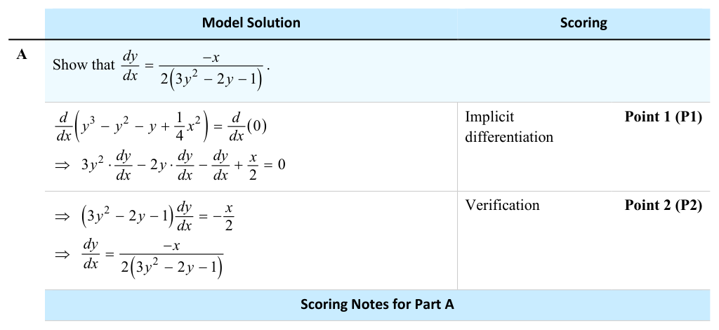
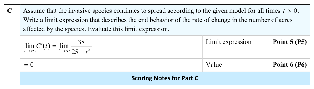
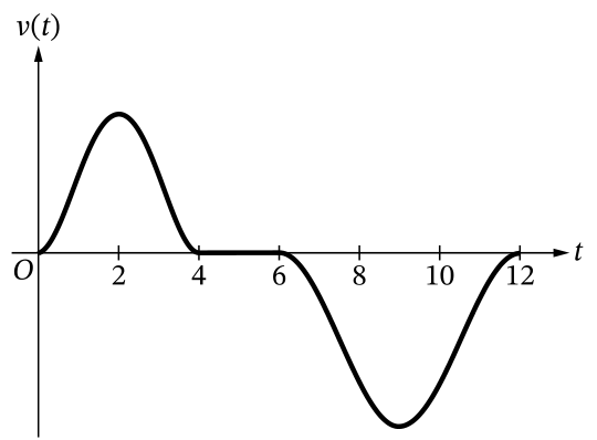
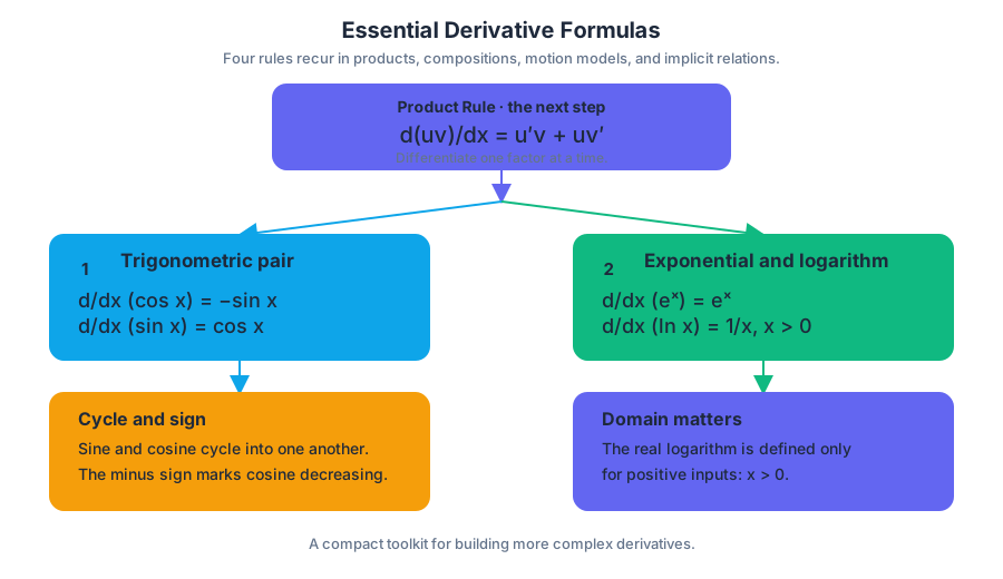
2.8 The Product Rule
Key concepts: The product rule for differentiable functions · The chain rule and its applications · Using the product rule in implicit differentiation · AP Exam assessment of derivative rules · Essential knowledge: derivatives of products can be found using the product rule · The quotient rule · Finding g′(2) and showing the work leading to the answer
The product rule (fg)' = f'g + fg', why f'g' is wrong, and how to apply the rule to repeated products, products with a chain-rule factor, and mixed x-y terms in implicit differentiation.
2.8 The Product Rule
A changing signal may combine several behaviors at once: a polynomial trend, exponential growth, and periodic oscillation. Differentiation handles such expressions by matching each function with its derivative and then using the product rule, which separates how each factor contributes to the total rate of change.
Enduring Understanding FUN-3: Recognizing opportunities to apply derivative rules can simplify differentiation.
The examples on this page use the basic derivatives from Topic 2.7: $\frac{d}{dx}(\sin x)=\cos x$, $\frac{d}{dx}(\cos x)=-\sin x$, $\frac{d}{dx}(e^x)=e^x$, and $\frac{d}{dx}(\ln x)=\frac{1}{x}$ for $x>0$.
Products: why one derivative is not enough
If $f$ and $g$ are differentiable, their product changes because both factors may change. The required rule is:
Product Rule, FUN-3.B.1
For differentiable functions $f$ and $g$, $$ (fg)'=f'g+fg'. $$
This supports Learning Objective FUN-3.B: Calculate derivatives of products and quotients of differentiable functions. Notice the two terms: first, $f$ changes while $g$ is held in the multiplying position; second, $g$ changes while $f$ remains. Writing only $f'g'$ incorrectly combines two rates that do not represent the product’s rate of change.
Worked example: evaluating $g'(2)$
Let
$$ g(x)=x^2e^x\cos x. $$
Treat this as a product of $x^2$ and $e^x\cos x$:
$$ g'(x)=2x(e^x\cos x)+x^2\frac{d}{dx}(e^x\cos x). $$
Apply the product rule again to the inner product:
$$ \frac{d}{dx}(e^x\cos x)=e^x\cos x-e^x\sin x. $$
Therefore,
$$ g'(x)=2xe^x\cos x+x^2e^x\cos x-x^2e^x\sin x, $$
so
$$ g'(x)=e^x\left[(2x+x^2)\cos x-x^2\sin x\right]. $$
At $x=2$,
$$ g'(2)=e^2\left[8\cos 2-4\sin 2\right]\approx -51.47. $$
The supporting work matters: it shows which factors were differentiated and where each product-rule term came from.
The chain rule inside these rules
The formulas above give derivatives of functions whose input is simply $x$. If the input is another function, use the chain rule: differentiate the outside function, keep the inside function, and multiply by the derivative of the inside.
Learning Objective FUN-3.C is to calculate derivatives of compositions of differentiable functions, supported by Essential Knowledge FUN-3.C.1: the chain rule provides a way to differentiate composite functions.
For a product such as
$$ y=e^{x^2}\sin(4x), $$
apply both rules:
$$ y'=e^{x^2}(2x)\sin(4x)+e^{x^2}\cos(4x)(4). $$
Misconception check — “differentiate each factor separately and multiply.” The expression $f'g'$ is not the derivative of $fg$. Use the product rule for multiplication and the chain rule for a function placed inside another function; an expression can require both.
Product rule in implicit differentiation
Implicit differentiation becomes essential when $y$ is not isolated. If a term contains both $x$ and $y$, differentiate it as a product and remember that $y$ depends on $x$.
For
$$ x^2y+\sin y=7, $$
differentiate with respect to $x$:
$$ 2xy+x^2\frac{dy}{dx}+\cos y\frac{dy}{dx}=0. $$
Collect the $\frac{dy}{dx}$ terms:
$$ \left(x^2+\cos y\right)\frac{dy}{dx}=-2xy, $$
so
$$ \frac{dy}{dx}=\frac{-2xy}{x^2+\cos y}. $$
The factor $x^2y$ requires the product rule; the term $\sin y$ requires the chain rule.
AP assessment lens
These ideas are assessed through FUN 2.7 and FUN 2.8, especially Skill 1.E: Apply appropriate mathematical rules or procedures, with and without technology. Pattern recognition also matters: identify whether the expression is a product, a composition, or both before calculating.
On free-response work, write the derivative rule clearly, preserve factors long enough to show the structure, and include units when the quantity represents a rate. A correct final number without supporting work may not demonstrate the reasoning required by the scoring rubric.
Retrieval check
Differentiate
$$ h(x)=x^3\ln(2x+1). $$
The expected structure is
$$ h'(x)=3x^2\ln(2x+1)+x^3\left(\frac{2}{2x+1}\right). $$
The first term comes from the product rule; the factor $\frac{2}{2x+1}$ comes from the chain rule.
2.9 The Quotient Rule
Key concepts: Quotient rule for differentiable functions · Calculating derivatives of quotients · Learning objective FUN-3.B · Essential knowledge FUN-3.B.2
The quotient rule for differentiating a ratio of two functions, a worked example with a rational function, and why differentiating the numerator and denominator separately fails.
2.9 The Quotient Rule
A quotient can change because both its numerator and denominator change. The quotient rule tracks those two effects without requiring the fraction to be expanded or rewritten first.
If $y=\dfrac{u(x)}{v(x)}$, where $u$ and $v$ are differentiable and $v(x)\neq 0$, then $$y'=\frac{v(x)u'(x)-u(x)v'(x)}{[v(x)]^2}.$$
The pattern is often remembered as “bottom times derivative of top, minus top times derivative of bottom, all over bottom squared.” The subtraction matters: reversing the two numerator terms changes the sign of the derivative.
The quotient rule in action
Suppose a sensor reports an efficiency ratio $$E(x)=\frac{3x^2+1}{x-2},$$ where $x$ represents an operating setting. The quotient rule is appropriate because both the numerator and denominator depend on $x$.
Let $$u(x)=3x^2+1,\qquad v(x)=x-2.$$ Then $$u'(x)=6x,\qquad v'(x)=1.$$ Substitute into the rule: $$ E'(x)=\frac{(x-2)(6x)-(3x^2+1)(1)}{(x-2)^2}. $$ Simplifying the numerator gives $$ E'(x)=\frac{6x^2-12x-3x^2-1}{(x-2)^2} =\frac{3x^2-12x-1}{(x-2)^2}. $$ The derivative is undefined at $x=2$, exactly where the original ratio is also undefined.
This example satisfies FUN-3.B: Calculate derivatives of products and quotients of differentiable functions and uses FUN-3.B.2: Derivatives of quotients of differentiable functions can be found using the quotient rule. The AP skill most directly involved is Skill 1.D: Identify an appropriate mathematical procedure, given information about a function or a function’s derivative. Here, recognizing a quotient leads directly to the quotient rule.
Products and quotients together
The examples in the rest of this page borrow two results from Topic 2.10: $\frac{d}{dx}[\tan(x)]=\sec^2(x)$ and $\frac{d}{dx}[\sec(x)]=\sec(x)\tan(x)$.
A function may require more than one rule. For $$F(x)=x^2\sec(x),$$ use the product rule: $$ F'(x)=2x\sec(x)+x^2\sec(x)\tan(x). $$ For $$G(x)=\frac{\tan(x)}{x^2+1},$$ use the quotient rule: $$ G'(x)=\frac{(x^2+1)\sec^2(x)-\tan(x)(2x)}{(x^2+1)^2}. $$
A common misconception is “differentiate the top and bottom separately”: $$ \left(\frac{u}{v}\right)'\neq\frac{u'}{v'}. $$ The quotient rule contains the cross-products $vu'$ and $uv'$, because changing either part affects the entire ratio.
Retrieval check
For $$H(x)=\frac{\sec(x)}{x+1},$$ identify the rule and write $H'(x)$ without expanding. Then state which identity would allow a derivation of $\sec'(x)$ from earlier derivative rules. The answers are
$$ H'(x)=\frac{(x+1)\sec(x)\tan(x)-\sec(x)}{(x+1)^2}, $$ and $$ \sec(x)=\frac{1}{\cos(x)}. $$
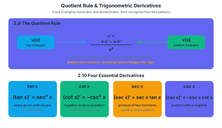
2.10 Derivatives of \(\tan x\), \(\cot x\), \(\sec x\), and \(\csc x\)
Key concepts: Derivatives of tan x · Derivatives of cot x · Derivatives of sec x · Derivatives of csc x · Using trigonometric identities to derive derivatives · Learning objective FUN-3.B
Deriving the derivatives of tan x, cot x, sec x and csc x by rewriting each as a quotient of sine and cosine, with the four resulting formulas and their sign patterns.
2.10 Derivatives of (\tan x), (\cot x), (\sec x), and (\csc x)
Tangent, cotangent, secant and cosecant are built from sine and cosine by division, so their derivatives need no new limits. Rewrite each one as a quotient, apply the quotient rule of Topic 2.9, $\left(\frac{u}{v}\right)'=\frac{vu'-uv'}{v^2}$, together with $\frac{d}{dx}[\sin(x)]=\cos(x)$ and $\frac{d}{dx}[\cos(x)]=-\sin(x)$, and simplify with $\sin^2(x)+\cos^2(x)=1$.
Trigonometric quotients
The trigonometric functions in Topic $2.10$ are connected by identities. Rewriting them exposes a product or quotient whose derivative can be calculated with rules already established:
$$ \tan(x)=\frac{\sin(x)}{\cos(x)},\qquad \cot(x)=\frac{\cos(x)}{\sin(x)}, $$
$$ \sec(x)=\frac{1}{\cos(x)},\qquad \csc(x)=\frac{1}{\sin(x)}. $$
This is FUN-3.B.3: Rearranging tangent, cotangent, secant, and cosecant functions using identities allows differentiation using derivative rules. The identity is not merely a memorization trick: it reveals which differentiation procedure applies.
Derivative of $\tan x$
Using $\tan(x)=\dfrac{\sin(x)}{\cos(x)}$, with numerator $\sin(x)$ and denominator $\cos(x)$,
$$ \frac{d}{dx}[\tan(x)] =\frac{\cos(x)\cos(x)-\sin(x)(-\sin(x))}{\cos^2(x)}. $$
The numerator becomes $$ \cos^2(x)+\sin^2(x)=1, $$ so $$ \boxed{\frac{d}{dx}[\tan(x)]=\sec^2(x)}. $$
Derivative of $\cot x$
Using $\cot(x)=\dfrac{\cos(x)}{\sin(x)}$,
$$ \frac{d}{dx}[\cot(x)] =\frac{\sin(x)(-\sin(x))-\cos(x)\cos(x)}{\sin^2(x)} =-\frac{\sin^2(x)+\cos^2(x)}{\sin^2(x)}. $$
Therefore, $$ \boxed{\frac{d}{dx}[\cot(x)]=-\csc^2(x)}. $$
Derivatives of $\sec x$ and $\csc x$
Write $\sec(x)=\dfrac{1}{\cos(x)}$. Applying the quotient rule gives
$$ \frac{d}{dx}[\sec(x)] =\frac{\cos(x)(0)-1(-\sin(x))}{\cos^2(x)} =\frac{\sin(x)}{\cos^2(x)} =\sec(x)\tan(x). $$
Likewise, $\csc(x)=\dfrac{1}{\sin(x)}$, so
$$ \frac{d}{dx}[\csc(x)] =\frac{\sin(x)(0)-1\cos(x)}{\sin^2(x)} =-\frac{\cos(x)}{\sin^2(x)} =-\csc(x)\cot(x). $$
The four essential formulas are therefore
$$ \boxed{\frac{d}{dx}[\tan(x)]=\sec^2(x)},\qquad \boxed{\frac{d}{dx}[\cot(x)]=-\csc^2(x)}, $$
$$ \boxed{\frac{d}{dx}[\sec(x)]=\sec(x)\tan(x)},\qquad \boxed{\frac{d}{dx}[\csc(x)]=-\csc(x)\cot(x)}. $$
Products and quotients together
A function may require more than one rule. For $$F(x)=x^2\sec(x),$$ use the product rule: $$ F'(x)=2x\sec(x)+x^2\sec(x)\tan(x). $$ For $$G(x)=\frac{\tan(x)}{x^2+1},$$ use the quotient rule: $$ G'(x)=\frac{(x^2+1)\sec^2(x)-\tan(x)(2x)}{(x^2+1)^2}. $$
A common misconception is “differentiate the top and bottom separately”: $$ \left(\frac{u}{v}\right)'\neq\frac{u'}{v'}. $$ The quotient rule contains the cross-products $vu'$ and $uv'$, because changing either part affects the entire ratio.
A second misconception concerns signs. The derivative of $\tan x$ is always positive where defined, and the derivative of $\cot x$ is always negative. The signs of $\sec x\tan x$ and $-\csc x\cot x$ depend on the interval, so their formulas must be used to determine the sign.
Retrieval check
For $$H(x)=\frac{\sec(x)}{x+1},$$ identify the rule and write $H'(x)$ without expanding. Then state which identity would allow a derivation of $\sec'(x)$ from earlier derivative rules. The answers are
$$ H'(x)=\frac{(x+1)\sec(x)\tan(x)-\sec(x)}{(x+1)^2}, $$ and $$ \sec(x)=\frac{1}{\cos(x)}. $$
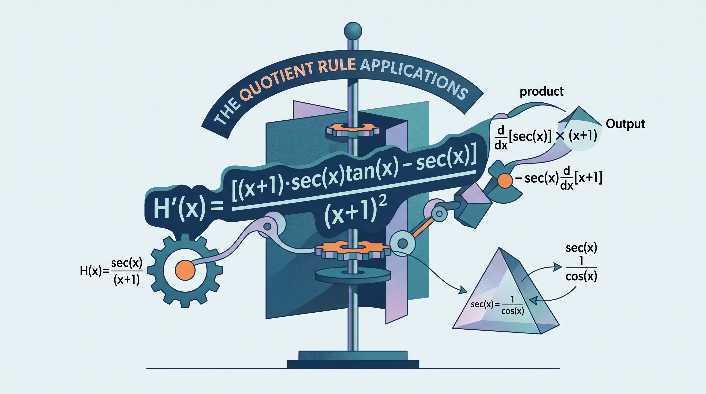
3.1 The Chain Rule
Key concepts: Composite functions · Identifying functions embedded within other functions · Decomposing composite functions · Chain rule · Differentiation of composite functions · Product rule · Quotient rule · Applying derivative rules strategically
How to recognize a composite function, name its inner and outer parts, and differentiate it with the chain rule, alone, in context, and alongside the product and quotient rules.
3.1 The Chain Rule
A temperature can change because time changes an inner quantity, which changes the temperature through an outer rule. The chain rule measures this linked change: differentiate the outside function, keep the inside function temporarily intact, then multiply by the derivative of the inside.
Composite functions: functions inside functions
A composite function is a function built by feeding one function into another. In $f(g(x))$, the function $g$ is the inner function and $f$ is the outer function. Recognizing this structure is the key decision before differentiating.
For example,
$$ y=\sin(3x^2+1) $$
has inner function $u=3x^2+1$ and outer function $y=\sin u$. The expression is not merely “a sine function”; its input is itself changing with $x$.
The chain rule is
$$ \frac{d}{dx}\left[f(g(x))\right] =f'(g(x))\cdot g'(x). $$
In words: differentiate the outer function at the inner input, then multiply by the derivative of the inner function.
Applying it gives
$$ \frac{dy}{dx} =\cos(3x^2+1)\cdot 6x =6x\cos(3x^2+1). $$
The inner expression remains visible until its derivative has been multiplied in.
A contextual example
Suppose a temperature model, in temperature units, is
$$ T(t)=10+\cos(2.4t), $$
where $t$ is measured in minutes. The outer function is cosine, and the inner function is $2.4t$:
$$ T'(t)=-\sin(2.4t)\cdot 2.4. $$
At $t=1$,
$$ T'(1)=-2.4\sin(2.4)\approx -1.621. $$
Thus, at one minute, the temperature is decreasing at approximately $1.621$ temperature units per minute. The negative sign describes direction; the units describe meaning.
The same chain-rule idea appears in equations, tables, and graphs. An equation may display the nested structure directly, a table may provide an inner rate and an outer derivative separately, and a graph may show how a change in one quantity produces a change in another. Practice 2—Connecting Representations is developed when these forms are interpreted as equivalent descriptions rather than separate procedures.
Choosing the correct derivative rule
Before differentiating, classify the expression. A sum uses the sum rule, a product uses the product rule, a quotient uses the quotient rule, and a composition uses the chain rule. Some expressions require several rules in sequence.
For a product,
$$ y=x^2\cos x, $$
the product rule gives
$$ y'=2x\cos x-x^2\sin x. $$
For a quotient,
$$ y=\frac{\sin x}{x^2+1}, $$
the quotient rule gives
$$ y'=\frac{(x^2+1)\cos x-\sin x(2x)}{(x^2+1)^2}. $$
A useful simplification is to rewrite expressions when that exposes a familiar rule. For instance,
$$ y=(x^2+1)^5 $$
is a power of a composite expression, so
$$ y'=5(x^2+1)^4(2x)=10x(x^2+1)^4. $$
Misconception check — “Differentiate only the visible outside.” Writing
$$ \frac{d}{dx}\sin(3x^2+1)=\cos(3x^2+1) $$
misses the fact that the input $3x^2+1$ also changes. The missing factor is $(3x^2+1)'=6x$.
Skills and retrieval check
This topic targets FUN-3.C—Calculate derivatives of compositions of differentiable functions—with FUN-3.C.1—The chain rule provides a way to differentiate composite functions. Suggested Skill 1.C is Identify an appropriate mathematical rule or procedure based on the classification of a given expression: decide whether an expression is a sum, a product, a quotient or a composition, and name its inner and outer functions, before differentiating. Topic 3.2 applies the same rule when the inner function is an unknown $y(x)$ inside an equation.
Retrieval check: Identify the inner and outer functions in $y=\ln(5x^3-2)$, then find $dy/dx$. Which factor in your answer is the derivative of the inner function, and what is lost if it is left out?
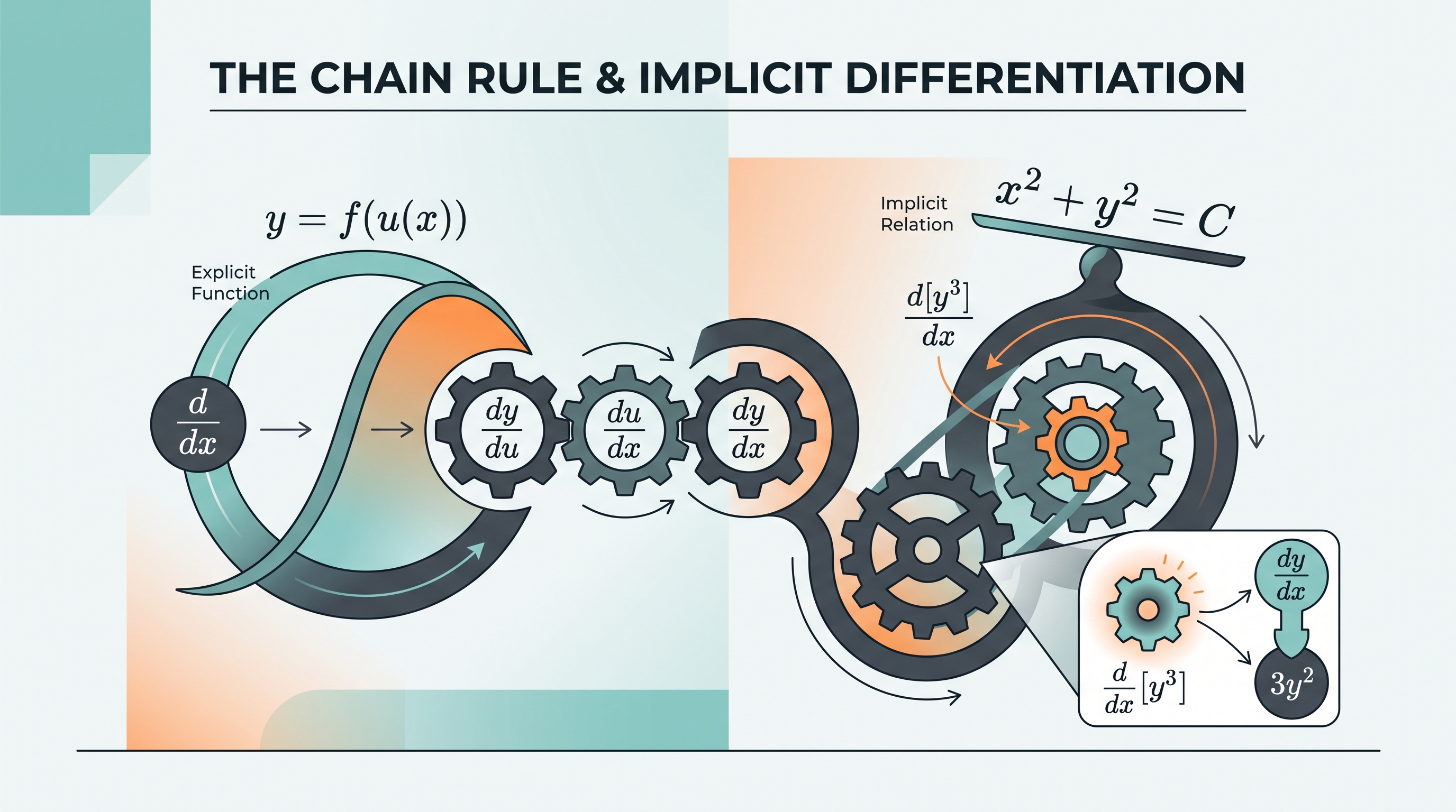
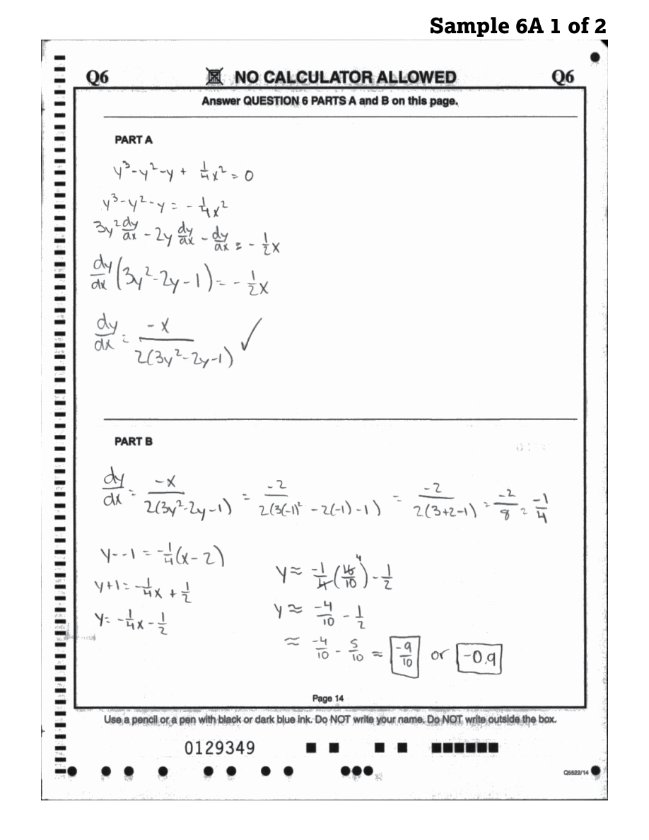
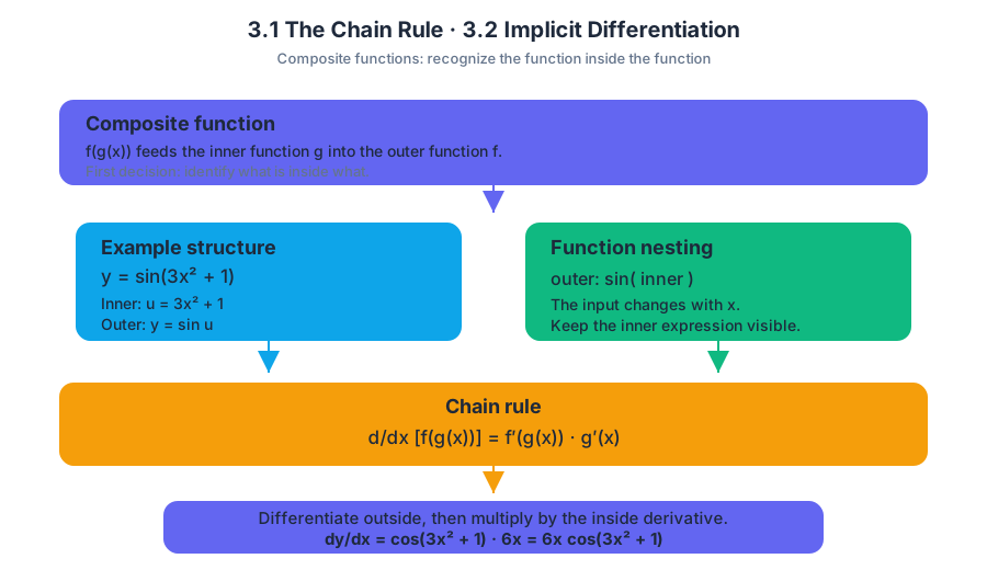
3.2 Implicit Differentiation
Key concepts: Implicit functions · Chain rule · Product rule · Differentiation of inverse functions · Applying derivative rules strategically
How to find $dy/dx$ for a curve defined by an equation in $x$ and $y$: differentiate both sides, attach $dy/dx$ to every $y$-term through the chain rule, then solve for the slope.
3.2 Implicit Differentiation
Many curves, such as circles and ellipses, are described by an equation that mixes $x$ and $y$ and cannot be solved neatly for a single $y=f(x)$. Implicit differentiation finds the slope $\frac{dy}{dx}$ of such a curve directly from its equation, by applying the chain rule from Topic 3.1 to every term that contains $y$.
Implicit differentiation: when $y$ is not isolated
An implicit function is defined by an equation relating $x$ and $y$, rather than by an equation already solved as $y=f(x)$. The circle
$$ x^2+y^2=25 $$
is an implicit relation. Solving first for $y$ would produce two branches, so implicit differentiation is usually cleaner.
Differentiate both sides with respect to $x$, remembering that $y$ depends on $x$:
$$ \frac{d}{dx}(x^2)+\frac{d}{dx}(y^2)=\frac{d}{dx}(25), $$
$$ 2x+2y\frac{dy}{dx}=0. $$
The factor $\frac{dy}{dx}$ appears because differentiating $y^2$ uses the chain rule: the outer function is $u^2$, while the inner function is $u=y(x)$.
Solving,
$$ \frac{dy}{dx}=-\frac{x}{y}. $$
At the point $(3,4)$, the tangent slope is
$$ \left.\frac{dy}{dx}\right|_{(3,4)}=-\frac34. $$
For a relation containing products, apply the product rule before collecting derivative terms. If
$$ x^2+xy+y^2=7, $$
then
$$ 2x+\left(x\frac{dy}{dx}+y\right)+2y\frac{dy}{dx}=0. $$
Collecting,
$$ (x+2y)\frac{dy}{dx}=-(2x+y), $$
so
$$ \frac{dy}{dx}=-\frac{2x+y}{x+2y}. $$
Implicit differentiation can also be used when the equation contains quotients; the quotient rule applies exactly as it does for explicit functions.
Skills and retrieval check
This topic targets FUN-3—Recognizing opportunities to apply derivative rules can simplify differentiation—especially FUN-3.C—Calculate derivatives of compositions of differentiable functions—with FUN-3.C.1—The chain rule provides a way to differentiate composite functions. It also targets FUN-3.D—Calculate derivatives of implicitly defined functions—with FUN-3.D.1—The chain rule is the basis for implicit differentiation. Suggested Skill 1.C is Identify an appropriate mathematical rule or procedure based on the classification of a given expression; Suggested Skill 1.E is Apply appropriate mathematical rules or procedures, with and without technology.
Retrieval check: Identify the inner function in $y=\ln(5x^3-2)$, then find $dy/dx$. For the implicit relation $x^3+y^3=16$, explain why differentiating $y^3$ produces $3y^2,dy/dx$ rather than merely $3y^2$.
3.3 Differentiating Inverse Functions
Key concepts: Differentiating inverse functions · Unit 3: Differentiation—composite, implicit, and inverse functions · Using differentiation and its inverse process · Checking the accuracy and appropriateness of solutions · Applying procedures with and without technology
How to find the derivative of an inverse function at a point from the original function's derivative, using reciprocal slopes at corresponding points, without solving for the inverse.
3.3 Differentiating Inverse Functions
If a function converts an input into an output, its inverse reverses that conversion: the inverse function answers, “Which input produced this output?” Differentiation reverses in the same spirit—but not by simply copying the original derivative.
The inverse-function derivative rule
Suppose $f$ is one-to-one, so that its inverse $f^{-1}$ exists. If $y=f(x)$ and $x=f^{-1}(y)$, then the slopes of the two graphs are reciprocal at corresponding points:
If $f$ is differentiable and $f'(f^{-1}(x))\ne0$, then
$$\left(f^{-1}\right)'(x)=\frac{1}{f'\left(f^{-1}(x)\right)}.$$
The notation matters: $f^{-1}(x)$ means the inverse function, not the reciprocal $\frac{1}{f(x)}$. The graphs of $f$ and $f^{-1}$ reflect across the line $y=x$; reflection exchanges horizontal and vertical change, which explains why the slopes become reciprocals.
Where the rule comes from. Because $f(f^{-1}(x))=x$, differentiating both sides with the chain rule gives $f'(f^{-1}(x))\cdot\left(f^{-1}\right)'(x)=1$. Dividing by $f'(f^{-1}(x))$, which must be nonzero, produces the rule above.
Worked example: reversing a calibration curve
A sensor converts an input temperature $x$ into a reading $f(x)=x^3+2x$. To recover temperature from a reading, define $g=f^{-1}$. Find $g'(3)$ without solving explicitly for $g$.
First locate the original input that produces the output $3$:
$$f(1)=1^3+2(1)=3,$$
so $g(3)=1$. Differentiate the original function:
$$f'(x)=3x^2+2.$$
Now apply the inverse-function rule at the corresponding point:
$$g'(3)=\frac{1}{f'(g(3))} =\frac{1}{f'(1)} =\frac{1}{3(1)^2+2} =\frac15.$$
The recovered-temperature function changes at $\frac15$ temperature units per sensor-reading unit when the reading is $3$. Notice that no explicit formula for $f^{-1}$ was required.
Checking an inverse-function derivative
Topic 3.3 explicitly assesses 3.G Confirm that solutions are accurate and appropriate. For an inverse-function derivative, check three things: $f'$ was evaluated at the matching input $f^{-1}(a)$, not at $a$ itself; $f'$ is nonzero there; and the sign is sensible, because an increasing $f$ has an increasing inverse. In the calibration example, $f'(1)=5$ and $g'(3)=\frac15$ multiply to $1$, as reciprocal slopes at corresponding points must.
The procedure represented by 1.E Apply appropriate mathematical rules or procedures, with and without technology requires both symbolic work and technology-supported verification. A graphing calculator can compare a numerical derivative or graph slope, but it does not replace identifying the correct inverse, domain, sign, or missing factor.
Retrieval check: Let $f(x)=x^3+x$ and $g=f^{-1}$. Given that $f(2)=10$, find $g(10)$ and $g'(10)$. Why does the answer use $f'(2)$ rather than $f'(10)$?
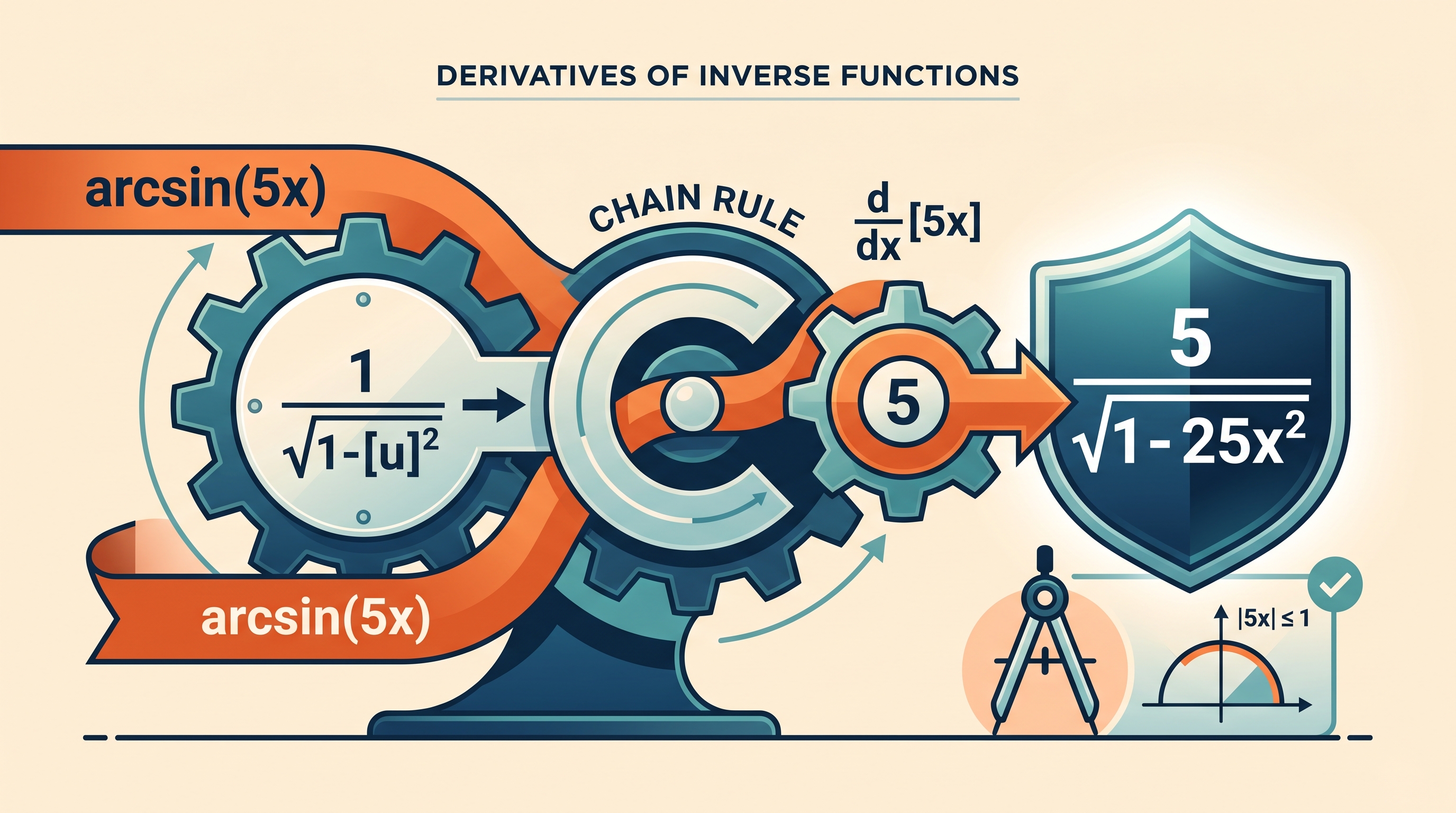
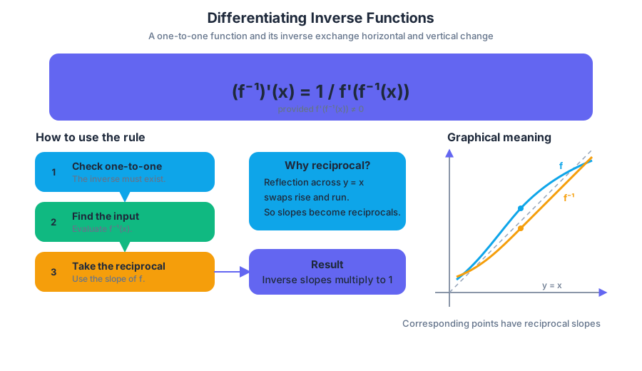
3.4 Differentiating Inverse Trigonometric Functions
Key concepts: Differentiating inverse trigonometric functions · Unit 3: Differentiation—composite, implicit, and inverse functions · Checking the accuracy and appropriateness of solutions · Applying procedures with and without technology · Differentiating compositions correctly · Identifying omitted or incorrectly differentiated composition components · Verifying that factors in an answer come from the original problem
The derivatives of $\arcsin x$, $\arccos x$ and $\arctan x$, where they come from, how to combine them with the chain rule, and how to check an answer's sign, inner factor and domain.
3.4 Differentiating Inverse Trigonometric Functions
Topic 3.3 showed that the slope of an inverse function is the reciprocal of the original function's slope at the corresponding point. Applying that idea to sine, cosine and tangent gives derivative formulas for $\arcsin x$, $\arccos x$ and $\arctan x$ that, surprisingly, contain no trigonometric functions at all.
Differentiating inverse trigonometric functions
The inverse trigonometric functions are restricted inverses of trigonometric functions. Restriction is essential because $\sin x$, $\cos x$, and $\tan x$ repeat values and therefore are not one-to-one on all real numbers.
On their standard domains and ranges, the derivative rules are:
| Function | Derivative |
|---|---|
| $y=\arcsin x$ | $\displaystyle \frac{dy}{dx}=\frac{1}{\sqrt{1-x^2}}$ |
| $y=\arccos x$ | $\displaystyle \frac{dy}{dx}=-\frac{1}{\sqrt{1-x^2}}$ |
| $y=\arctan x$ | $\displaystyle \frac{dy}{dx}=\frac{1}{1+x^2}$ |
For a composition, the derivative includes the derivative of the inside expression. For example, with $y=\arctan(3x^2)$,
$$\frac{dy}{dx} =\frac{1}{1+(3x^2)^2}\cdot 6x =\frac{6x}{1+9x^4}.$$
The factor $6x$ is not optional: it records how quickly the input $3x^2$ changes.
A geometric check for $\arcsin x$
Let $y=\arcsin x$. Then $\sin y=x$, with $-\frac{\pi}{2}\le y\le\frac{\pi}{2}$. Differentiating gives
$$\cos y\frac{dy}{dx}=1,$$
so
$$\frac{dy}{dx}=\frac{1}{\cos y}.$$
Because $\cos y\ge0$ on this restricted range and $\sin y=x$,
$$\cos y=\sqrt{1-\sin^2y}=\sqrt{1-x^2},$$
therefore
$$\frac{d}{dx}(\arcsin x)=\frac{1}{\sqrt{1-x^2}}.$$
The square root is required. Replacing it with $\cos^{-1}x$ would confuse an inverse function with a reciprocal and would produce the wrong expression.
Accuracy and appropriateness checks
Topic 3.3 and Topic 3.4 explicitly assess 3.G Confirm that solutions are accurate and appropriate. A reliable check asks three questions:
- Does the answer contain only factors from the original function and its differentiation rules?
- Was every composition differentiated, including the inside expression?
- Does the result fit the domain and sign of the function?
For instance, a proposed derivative of $\arccos(2x)$ equal to $\frac{1}{\sqrt{1-4x^2}}$ is incorrect because the inner derivative $2$ was skipped and the sign is wrong. The correct result is
$$-\frac{2}{\sqrt{1-4x^2}}.$$
A proposed answer with an unexplained factor such as $7$ should also be rejected: that factor did not arise from the original expression.
Misconception check: $\arctan x$ is not $\frac{1}{\tan x}$, and $\arcsin x$ is not $\frac{1}{\sin x}$. The prefix “arc” identifies an inverse function.
The procedure represented by 1.E Apply appropriate mathematical rules or procedures, with and without technology requires both symbolic work and technology-supported verification. A graphing calculator can compare a numerical derivative or graph slope, but it does not replace identifying the correct inverse, domain, sign, or missing factor.
Retrieval check
Find $\dfrac{d}{dx}\left[\arcsin(5x)\right]$ and explain one check that supports your answer.
The result is
$$\frac{5}{\sqrt{1-25x^2}}.$$
The factor $5$ comes from differentiating the inside expression $5x$, and the denominator requires $|5x|\le1$, confirming that the formula is appropriate on the real domain.
3.5 Selecting Procedures for Calculating Derivatives
Key concepts: Selecting an appropriate differentiation procedure · Differentiation rules for composite functions · The chain rule · Applying derivative rules with and without technology · Checking derivative answers and notation · Explaining and justifying the choice of a derivative procedure · Recognizing and correcting differentiation errors
How to classify an expression as a power, sum, product, quotient or composition so the right derivative rule is chosen, with the chain rule worked layer by layer and checked with technology.
3.5 Selecting Procedures for Calculating Derivatives
A derivative problem is often decided before any algebra begins: the expression’s structure tells you which rule belongs. A function such as $y=(x^2+1)^3$ is not merely a power; it is a composite function, an outer power applied to an inner quadratic.
Choosing the procedure
Selecting an appropriate differentiation procedure means classifying the expression before differentiating it. Ask what operation connects the visible pieces:
| Expression structure | Appropriate procedure |
|---|---|
| $y=x^n$ | Power Rule |
| $y=u(x)+v(x)$ | Sum Rule |
| $y=c,u(x)$ | Constant Multiple Rule |
| $y=u(x)v(x)$ | Product Rule |
| $y=\dfrac{u(x)}{v(x)}$ | Quotient Rule |
| $y=f(g(x))$ | Chain Rule |
The relevant AP skill is 1.C Identify an appropriate mathematical rule or procedure based on the classification of a given expression. Topic 3.5 is specifically intended to develop this selection skill, while also requiring accurate application of derivative procedures with and without technology.
The chain rule: differentiate each layer
The chain rule differentiates a composite function by multiplying the derivative of the outer function by the derivative of the inner function. In symbols, if $y=f(g(x))$, then
$$ \frac{dy}{dx}=f'(g(x))\cdot g'(x). $$
A useful visual is a two-stage machine:
$$ x \longrightarrow g(x) \longrightarrow f(g(x)). $$
Differentiate by moving backward through the machine:
$$ \text{outer derivative}\times\text{inner derivative}. $$
Worked example. Let
$$ y=(x^2+1)^3. $$
The inner function is $u=x^2+1$, and the outer function is $u^3$. Differentiate the outer layer while keeping the inner expression intact, then multiply by the derivative of the inner layer:
$$ \frac{dy}{dx}=3(x^2+1)^2(2x) =6x(x^2+1)^2. $$
The same structure applies to trigonometric, exponential, and logarithmic compositions. For example,
$$ y=\sin(4x^2) $$
has outer function $\sin u$ and inner function $u=4x^2$, so
$$ \frac{dy}{dx}=\cos(4x^2)\cdot 8x =8x\cos(4x^2). $$
A technology check
A graphing calculator or computer algebra system can check a derivative, but it does not replace the mathematical procedure or notation. Enter the function $y=(x^2+1)^3$ and request its symbolic derivative. A CAS may return
$$ 3(x^2+1)^2(2x), $$
while handwritten work may give
$$ 6x(x^2+1)^2. $$
These expressions are equivalent because $3(2x)=6x$. To verify numerically, evaluate both at $x=1$:
$$ 3(1^2+1)^2(2)=24, \qquad 6(1)(1^2+1)^2=24. $$
A graphing calculator can also approximate the slope of $y=(x^2+1)^3$ near $x=1$; the result should be close to $24$. Check three things: the function was entered correctly, the derivative uses the correct variable, and the output is algebraically equivalent—not merely visually similar.
Misconception check — “Differentiate only the outside.” Writing
$$ \frac{d}{dx}(x^2+1)^3=3(x^2+1)^2 $$
stops after the outer derivative. The missing factor, $2x$, is the derivative of the inside. Without it, the chain is broken.
Classifying first matters just as much in Topic 3.6, where a derivative such as $y'$ is differentiated again to give the second derivative, written $y''$.
Retrieval check
For $y=\ln(5x^2+1)$, identify the procedure and calculate $\dfrac{dy}{dx}$. Then state why a factor of $10x$ must appear. Finally, if $y'=10x/(5x^2+1)$, write $y''$ using $y''$ notation. The essential habit is: classify first, differentiate layer by layer, and check both the mathematics and the notation.
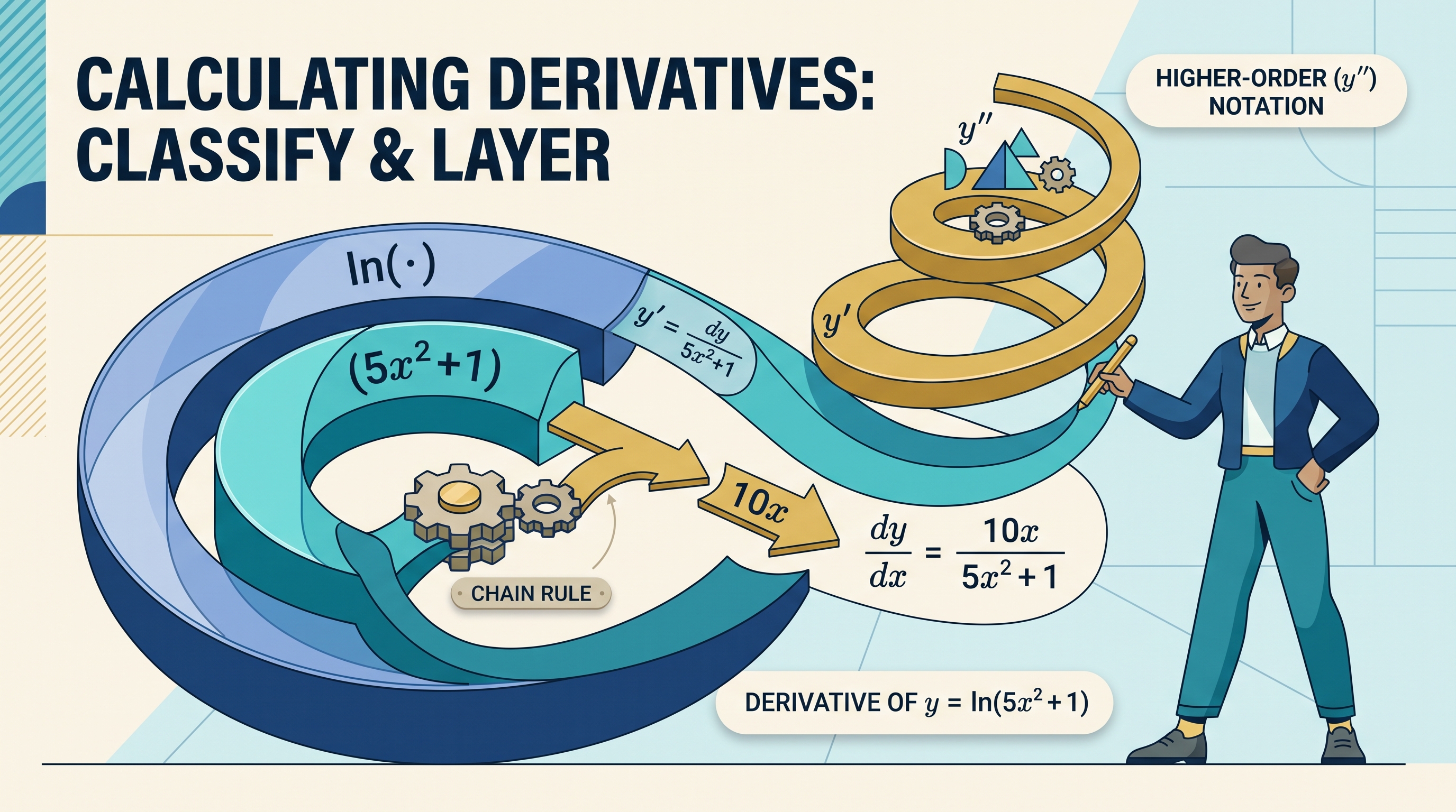
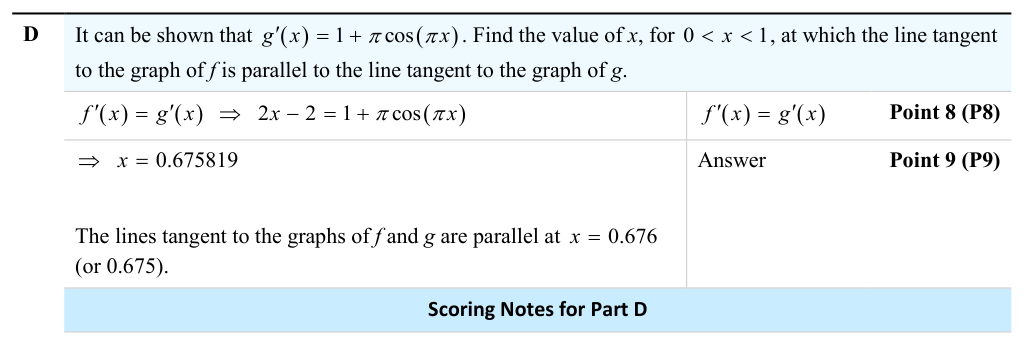
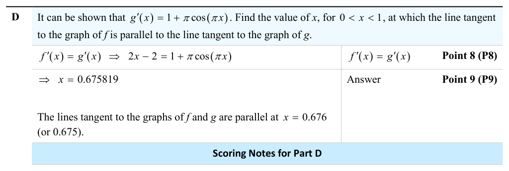
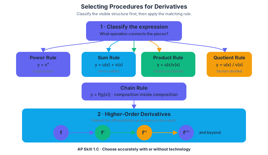
3.6 Calculating Higher-Order Derivatives
Key concepts: Checking derivative answers and notation · Higher-order derivatives · Second-derivative notation · General nth-derivative notation
How to find second, third and $n$th derivatives by differentiating repeatedly, and how to read and write the notation $y''$, $f^{(n)}(x)$ and $\frac{d^2y}{dx^2}$ correctly.
3.6 Calculating Higher-Order Derivatives
A derivative is itself a function, so it can be differentiated again. The result, the second derivative, measures how a rate of change is itself changing: if position has velocity as its first derivative, then acceleration is its second. This page shows how to calculate these repeated derivatives with the rules selected in Topic 3.5, and how to write them correctly.
Higher-order derivatives
A higher-order derivative is found by differentiating a derivative again. If $y=f(x)$, then the first derivative is $y'$ or $\dfrac{dy}{dx}$, and the second derivative is
$$ y''=\frac{d^2y}{dx^2}. $$
More generally, the $n$th derivative is written as
$$ f^{(n)}(x) \qquad\text{or}\qquad \frac{d^ny}{dx^n}. $$
For
$$ y=x^4-3x^2+2x, $$
the first derivative is
$$ y'=4x^3-6x+2, $$
and differentiating again gives
$$ y''=12x^2-6. $$
A third derivative is
$$ y'''=24x, $$
and the fourth derivative is
$$ y^{(4)}=24. $$
The notation communicates what has happened: $\dfrac{d^2y}{dx^2}$ means “differentiate twice with respect to $x$,” not $\left(\dfrac{dy}{dx}\right)^2$. In applications, $y'$ can represent a rate of change, while $y''$ describes how that rate itself changes. Repeated differentiation uses the same rules as the first derivative.
A second derivative that needs more than the power rule. Topic 3.5 found that $y=(x^2+1)^3$ has $y'=6x(x^2+1)^2$. That derivative is a product whose second factor is a composition, so differentiating again takes the product rule and the chain rule together: $y''=6(x^2+1)^2+6x\cdot 2(x^2+1)(2x)=6(x^2+1)(5x^2+1)$.
Retrieval check
For $y=\ln(5x^2+1)$, identify the procedure and calculate $\dfrac{dy}{dx}$. Then state why a factor of $10x$ must appear. Finally, if $y'=10x/(5x^2+1)$, write $y''$ using $y''$ notation. The essential habit is: classify first, differentiate layer by layer, and check both the mathematics and the notation.
4.1 Interpreting the Meaning of the Derivative in Context
Key concepts: Interpreting the derivative in context · Derivative as a rate of change · Careful reading of contextual language such as “find the rate of change” · Real-world applications of derivatives · Using representations to describe changing quantities
How to read a derivative in a real-world setting as an instantaneous rate, stating the quantity, the instant, the direction of change and the units.
4.1 Interpreting the Meaning of the Derivative in Context
A derivative measures how quickly one quantity changes with respect to another at a particular instant. If $C(t)$ represents acres affected by an invasive species, then $C'(t)$ tells how rapidly the affected area is changing at time $t$—not merely how much area exists.
The derivative is a rate with meaning and units
This topic belongs to CHA-3: Derivatives allow us to solve real-world problems involving rates of change. Its essential knowledge says a derivative is the instantaneous rate of change of a function with respect to its independent variable, that it expresses information about rates of change in applied contexts, and that the unit for $f'(x)$ is the unit for $f$ divided by the unit for $x$.
A phrase such as “find the rate of change of…” is a strong cue to use a derivative. The units of the derivative come from dividing the units of the output by the units of the input:
$$ \text{units of } f'(t)=\frac{\text{units of }f}{\text{units of }t}. $$
For example, suppose $C(t)=7.6\arctan(0.2t)$ measures acres affected $t$ weeks after an invasive species appears. If
$$ C'(t)=\frac{38}{25+t^2}, $$
then at $t=3$,
$$ C'(3)=\frac{38}{25+3^2}=\frac{38}{34}\approx 1.118. $$
The correct interpretation is: three weeks after appearing, the affected area is increasing at approximately $1.118$ acres per week. The answer is not $1.118$ acres, because $C'(3)$ measures a rate, not an amount.
A reliable interpretation pattern
When interpreting a derivative in context, identify four parts:
- Quantity: What does the function measure?
- Instant: At what input value is the derivative evaluated?
- Change: Is the quantity increasing or decreasing?
- Units: What units result from output units divided by input units?
The sign matters. If $f'(a)>0$, the quantity is increasing at the instant $a$. If $f'(a)<0$, it is decreasing. If $f'(a)=0$, the quantity has zero instantaneous rate of change—but this alone does not prove that the quantity is at a maximum or minimum.
Misconception check — “decreasing” versus “decreasing faster.” If $f'(t)<0$, then $f$ is decreasing. If $f''(t)<0$, then the rate $f'(t)$ is decreasing. These are different claims: a quantity can still be increasing while its rate of increase becomes smaller.
Choosing the procedure from the wording
The suggested skill for Topic 4.1 is 1.D: Identify an appropriate mathematical rule or procedure based on the relationship between concepts. In this setting, the relationship is “rate of change means derivative,” so a contextual phrase determines the procedure.
Retrieval check: $W(t)$ is the volume of water in a tank, in gallons, $t$ minutes after a valve opens. What are the units of $W'(t)$? If $W'(10)=-3$, state its meaning in context.
Answer: $W'(t)$ is measured in gallons per minute. The value $W'(10)=-3$ means that $10$ minutes after the valve opens, the volume of water in the tank is decreasing at $3$ gallons per minute.
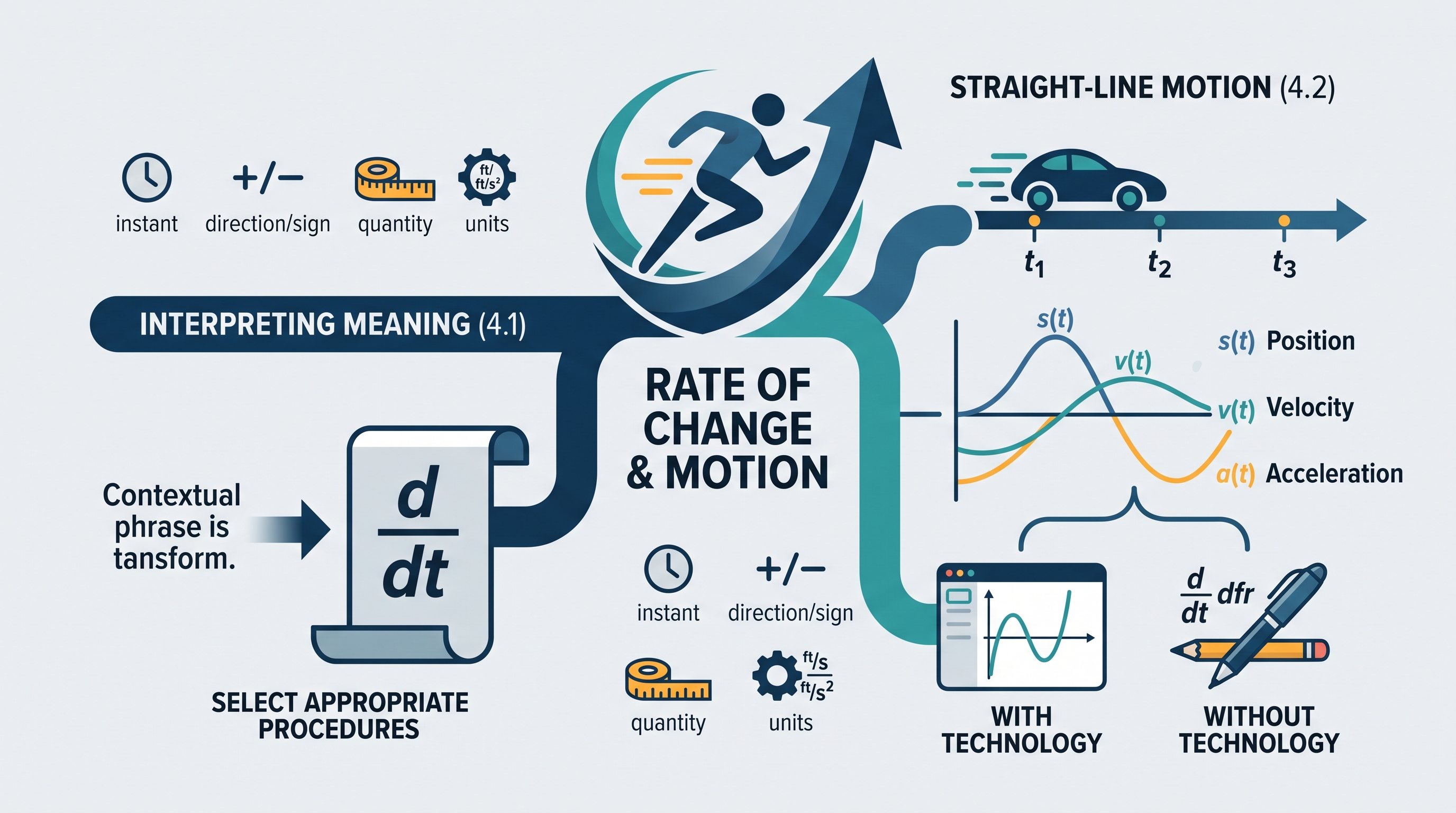
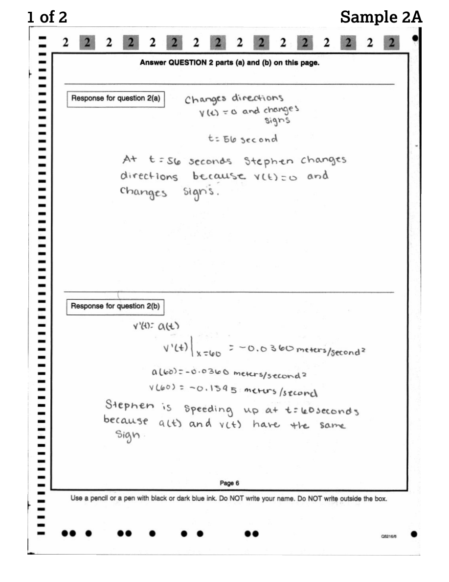
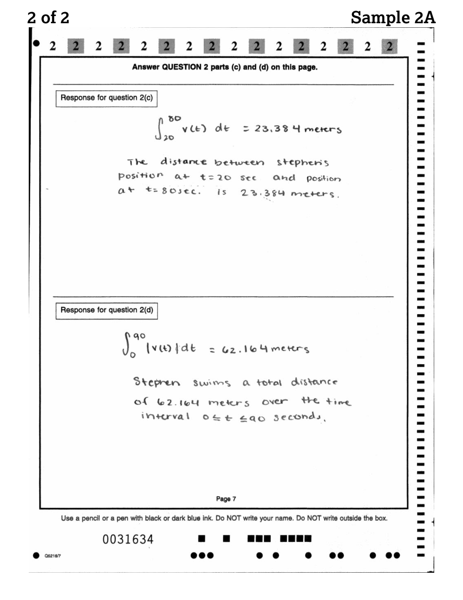
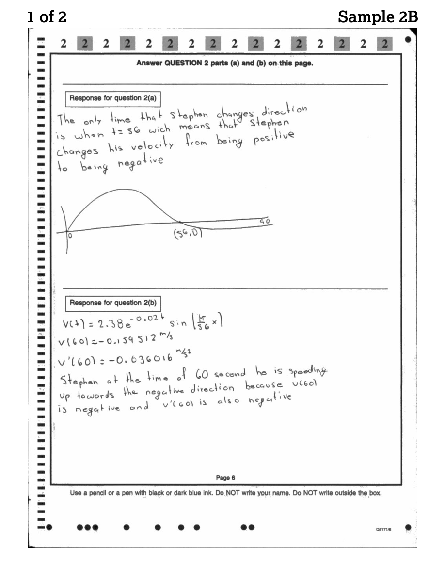
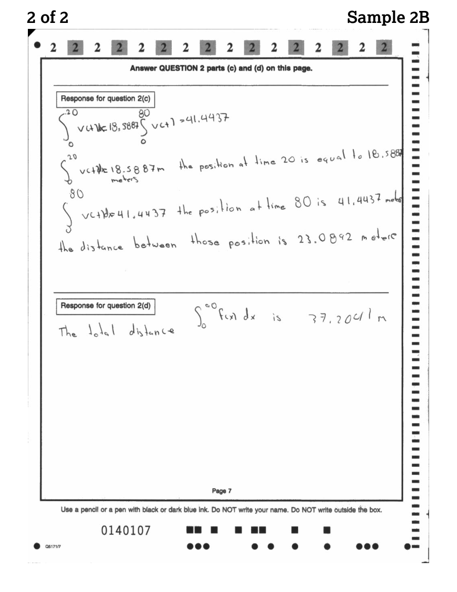
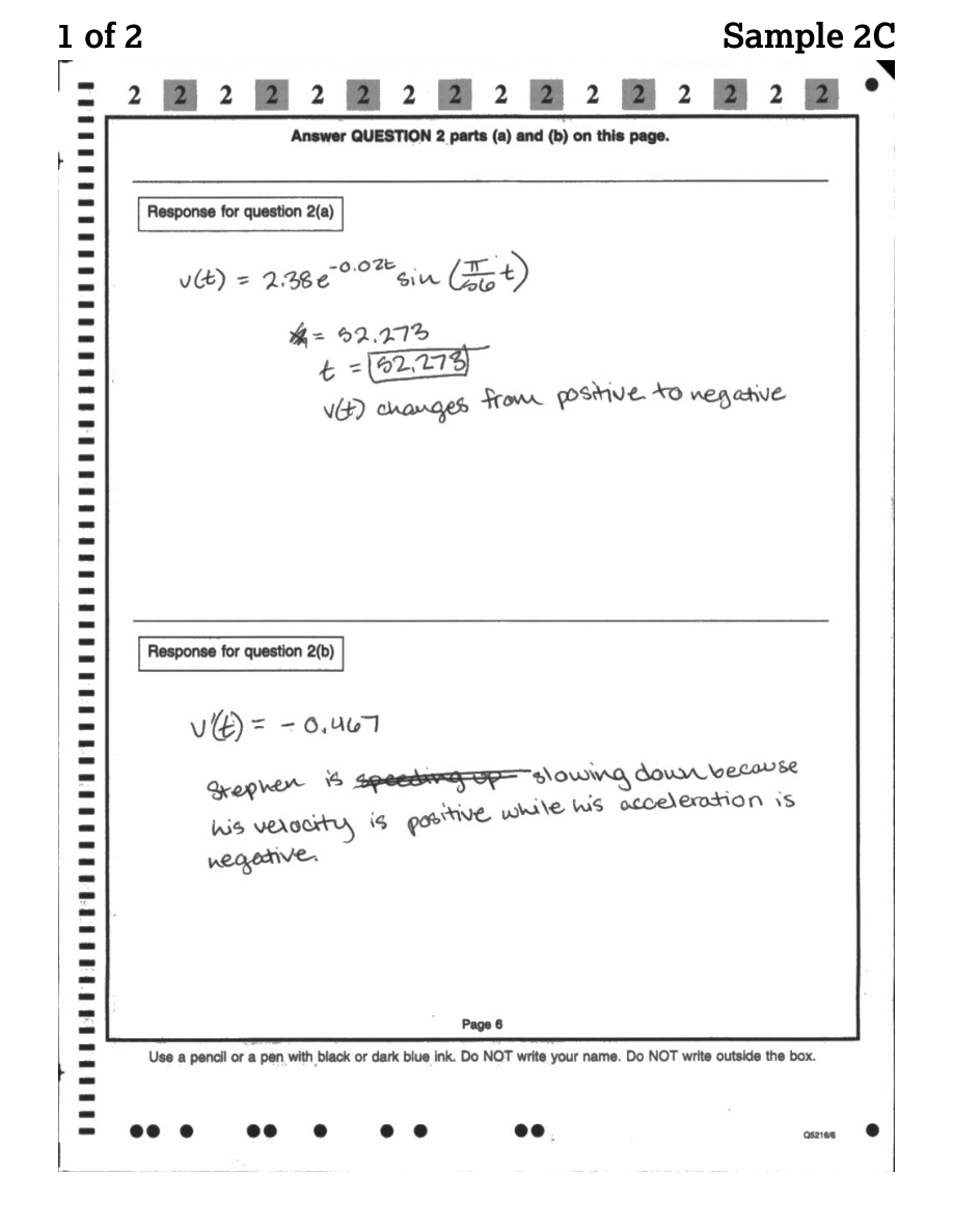
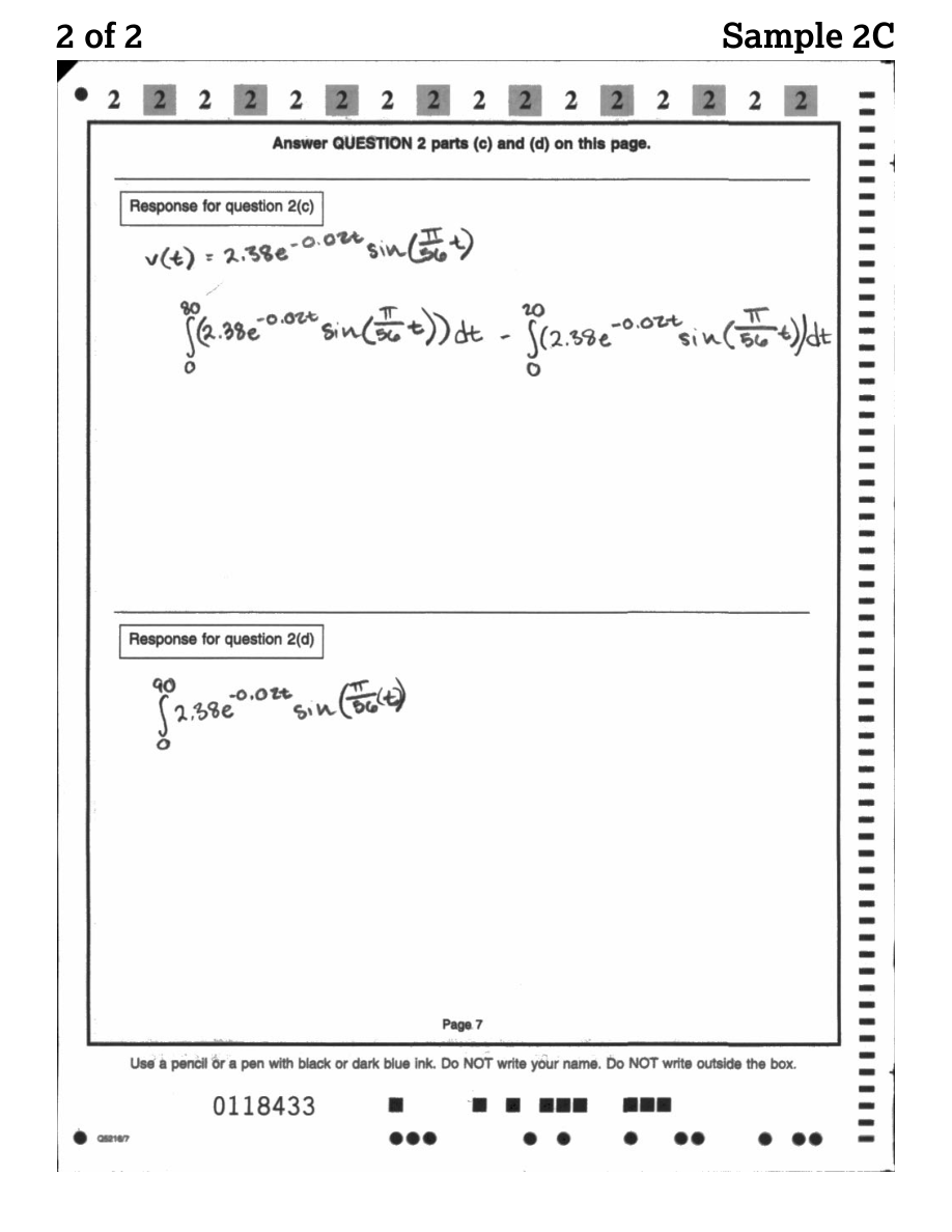
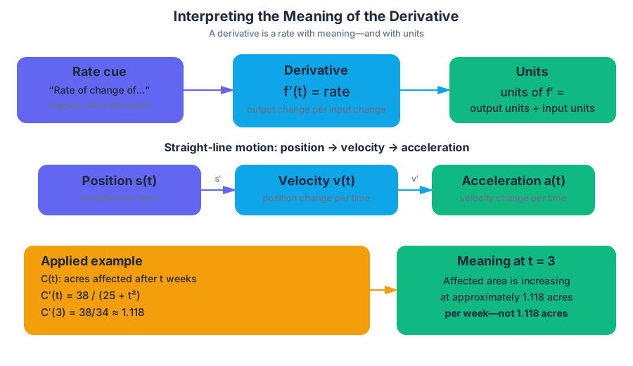
4.2 Straight-Line Motion: Connecting Position, Velocity, and Acceleration
Key concepts: Real-world applications of derivatives · Straight-line motion · Connections among position, velocity, and acceleration · Applying appropriate mathematical rules and procedures · Using representations to describe changing quantities
How the position, velocity and acceleration of a particle on a line are linked by derivatives, and how the sign of velocity gives the direction of motion.
4.2 Straight-Line Motion: Connecting Position, Velocity, and Acceleration
When the changing quantity is the position of an object moving along a line, its derivatives have names of their own. Velocity is the rate of change of position and acceleration is the rate of change of velocity, so everything Topic 4.1 says about reading a derivative, with its sign, instant and units, applies directly to motion.
The enduring understanding for these topics is CHA-3: Derivatives allow us to solve real-world problems involving rates of change. The learning objective is CHA-3.B: Calculate rates of change in applied contexts. Its essential knowledge, CHA-3.B.1, states that the derivative can solve rectilinear-motion problems involving position, speed, velocity, and acceleration.
Straight-line motion: position, velocity, and acceleration
For a particle moving along a line, let $s(t)$ denote its position at time $t$. Position gives location relative to a chosen origin. Its first derivative is velocity:
$$ v(t)=s'(t), $$
and the derivative of velocity is acceleration:
$$ a(t)=v'(t)=s''(t). $$
| Quantity | Meaning | Mathematical relationship | Typical units |
|---|---|---|---|
| Position $s(t)$ | Location on the line | Given function | meters |
| Velocity $v(t)$ | Signed rate of position change | $s'(t)$ | meters per second |
| Speed | Magnitude of velocity | $\lvert v(t)\rvert$ | meters per second |
| Acceleration $a(t)$ | Rate of velocity change | $v'(t)=s''(t)$ | meters per second squared |
Velocity is signed, so it describes both how fast and which direction. A particle moves right when $v(t)>0$ and left when $v(t)<0$. Speed is never negative because it is $\lvert v(t)\rvert$.
Worked motion example
A particle moves along the $x$-axis with position
$$ x(t)=t^3-6t^2+9t, $$
where $x$ is measured in meters and $t$ in seconds. Differentiate:
$$ v(t)=x'(t)=3t^2-12t+9, $$
$$ a(t)=v'(t)=6t-12. $$
At $t=1$,
$$ v(1)=3-12+9=0, $$
so the particle is momentarily at rest. Its acceleration is
$$ a(1)=6(1)-12=-6\ \text{m/s}^2. $$
At $t=3$,
$$ v(3)=27-36+9=0, $$
so the particle is again at rest. To determine direction, factor velocity:
$$ v(t)=3(t-1)(t-3). $$
Thus $v(t)>0$ on $0<t<1$, $v(t)<0$ on $1<t<3$, and $v(t)>0$ for $t>3$. The particle moves right, then left, then right again.
Applying procedures with and without technology
The suggested skill for Topic 4.2 is 1.E: Apply appropriate mathematical rules or procedures, with and without technology. A graphing calculator may help graph $s(t)$, $v(t)$, and $a(t)$ or estimate a derivative numerically, but the interpretation must still include a sign, an instant, a quantity, and units.
Retrieval check: If $s(t)$ is measured in feet and $t$ in seconds, what do $s'(4)$ and $s''(4)$ measure? If $s'(4)=-12$, state its meaning in context.
Answer: $s'(4)$ is velocity in feet per second; $s''(4)$ is acceleration in feet per second squared. The value $s'(4)=-12$ means that at $t=4$ seconds, the particle is moving in the negative direction at $12$ feet per second.
4.3 Rates of Change in Applied Contexts Other Than Motion
Key concepts: Rates of change in applied contexts other than motion · Applying derivatives to quantities other than time · Identifying common underlying structures across contextual problems · Connecting algebraic derivatives to real-world rates of change
How a derivative describes change in settings other than motion, such as population, cost or concentration, including inputs other than time, with correct units.
4.3 Rates of Change in Applied Contexts Other Than Motion
A derivative measures how one quantity changes as another quantity changes, whether the quantities describe motion, population, chemical concentration, revenue, or the size of a biological habitat. The input does not have to be time: if population $P$ depends on food supply $F$, then $\dfrac{dP}{dF}$ measures population change per unit of food supply.
From motion to every changing quantity
The essential structure is always a changing output compared with a changing input:
$$ \text{rate of change}=\frac{\text{change in dependent quantity}}{\text{change in independent quantity}}. $$
For example, suppose the population $P$ of a fish species depends on the available food supply $F$. If
$$ P=120+4F^2, $$
then differentiating with respect to $F$ gives
$$ \frac{dP}{dF}=8F. $$
At a food supply of $F=5$ units,
$$ \frac{dP}{dF}=8(5)=40. $$
The population is increasing at approximately $40$ fish per additional unit of food supply when $F=5$. The units are fish per food-supply unit, not fish per unit of time.
The same steps work in economics. If $C(q)=500+12q+0.02q^2$ is the cost in dollars of producing $q$ units, then $C'(q)=12+0.04q$ and $C'(100)=16$. When $100$ units are being produced, cost is increasing at about $16$ dollars per additional unit, a rate economists call the marginal cost.
This is Topic 4.3 Rates of Change in Applied Contexts Other Than Motion, aligned with Enduring Understanding CHA-3: Derivatives allow us to solve real-world problems involving rates of change, Learning Objective CHA-3.C: Interpret rates of change in applied contexts, and Essential Knowledge CHA-3.C.1: The derivative can be used to solve problems involving rates of change in applied contexts.
The associated Connecting Representations skill 2.A: Identify common underlying structures in problems involving different contextual situations asks you to recognize that a chemistry problem about concentration, an economics problem about cost, and a biology problem about population can share the same mathematical pattern. First identify the input and output; then differentiate the relationship and attach meaningful units.
Retrieval check: The concentration of a drug in the bloodstream is $D(t)$ milligrams per liter, $t$ hours after a dose. What are the units of $D'(t)$, and what does $D'(2)=-0.8$ mean? The units are milligrams per liter per hour; two hours after the dose, the concentration is decreasing at $0.8$ milligrams per liter per hour.
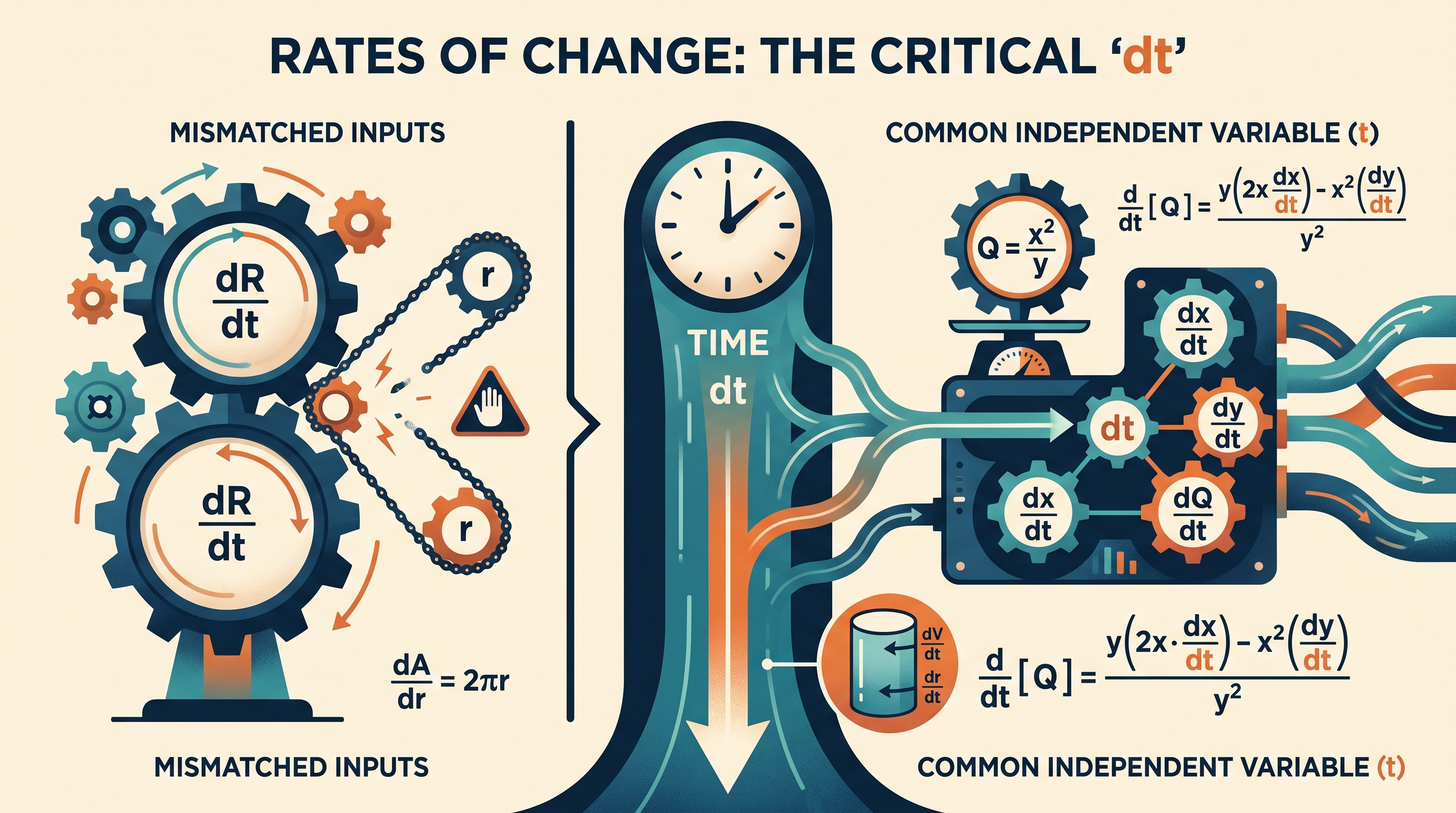
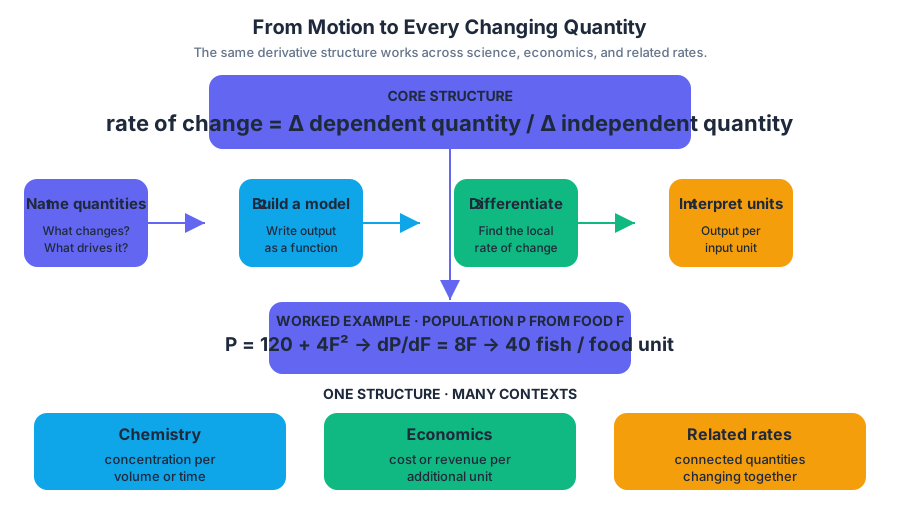
4.4 Introduction to Related Rates
Key concepts: Introduction to related rates · Using a common independent variable for multiple changing quantities · Interpreting related rates in applied contexts · Applying appropriate differentiation rules · Implicit differentiation in applied contexts · Geometric interpretation of derivatives as slopes
How to set up a related-rates problem: link the quantities with an equation, differentiate everything with respect to time using the chain rule, then substitute.
4.4 Introduction to Related Rates
Topic 4.3 used a derivative to describe how one quantity responds to another. In many applied problems several quantities change at once, all as time passes, and a known rate for one of them determines the rate for another. These are related-rates problems, and the chain rule is what links the rates.
Related rates: several quantities, one independent variable
A related-rates problem involves two or more quantities that change together because an equation connects them. Although time is the most common independent variable, every changing quantity must be differentiated with respect to the same independent variable. In applications, that variable is usually $t$.
Imagine a circular chemical spill whose radius $r$ changes as the spill spreads. Its area is
$$ A=\pi r^2. $$
If the radius grows at $\dfrac{dr}{dt}=0.6$ meters per minute when $r=10$ meters, differentiate both sides with respect to $t$:
$$ \frac{dA}{dt}=2\pi r\frac{dr}{dt}. $$
Substitute the known values:
$$ \frac{dA}{dt}=2\pi(10)(0.6)=12\pi\ \text{m}^2/\text{min}. $$
Thus, at that instant, the contaminated area is increasing at $12\pi$ square meters per minute. The factor $\dfrac{dr}{dt}$ appears because $r$ itself depends on $t$; this is the chain rule in action.
Topic 4.4 Introduction to Related Rates is aligned with Learning Objective CHA-3.D: Calculate related rates in applied contexts and Essential Knowledge CHA-3.D.1: The chain rule is the basis for differentiating variables in a related rates problem with respect to the same independent variable. The related-rates workflow is:
- Name the variables and their units.
- Write an equation relating the quantities.
- Differentiate the entire equation with respect to the common independent variable, usually $t$.
- Substitute values only after differentiating.
- Interpret the resulting rate, including its sign and units.
Implicit differentiation in an applied relationship
Sometimes the relationship between quantities is not solved explicitly for one variable. Consider a chemical process in which concentration variables $x$ and $y$ satisfy
$$ 6xy=2+y^3. $$
Suppose both concentrations change as time $t$ passes. Differentiate implicitly with respect to $t$:
$$ 6\left(x\frac{dy}{dt}+y\frac{dx}{dt}\right) =3y^2\frac{dy}{dt}. $$
Collect the terms containing $\dfrac{dy}{dt}$:
$$ 6x\frac{dy}{dt}-3y^2\frac{dy}{dt} =-6y\frac{dx}{dt}, $$
so
$$ \frac{dy}{dt}
\frac{-6y,\dfrac{dx}{dt}}{6x-3y^2}. $$
If $x=1$, $y=2$, and $\dfrac{dx}{dt}=0.05$ concentration units per minute, then
$$ \frac{dy}{dt}
\frac{-6(2)(0.05)}{6(1)-3(2)^2}
\frac{-0.6}{-6}
0.1. $$
Therefore, $y$ is increasing at $0.1$ concentration units per minute at that instant. The sign matters: the equation forces $y$ to rise while $x$ rises at the stated point.
If the same equation is viewed geometrically rather than chemically, differentiating with respect to $x$ gives
$$ 6\left(x\frac{dy}{dx}+y\right)=3y^2\frac{dy}{dx}, $$
and therefore
$$ \frac{dy}{dx}=\frac{-6y}{6x-3y^2}. $$
This derivative is the slope of the curve at the point $(x,y)$. Replacing $\dfrac{dy}{dx}$ with $\dfrac{dy/dt}{dx/dt}$ produces the same relationship when both variables change with time.
Rules and reasoning that prevent errors
The chain rule is not the only rule that may be required. Essential Knowledge CHA-3.D.2: Other differentiation rules, such as the product rule and the quotient rule, may also be necessary to differentiate all variables with respect to the same independent variable. For instance, if
$$ Q=\frac{x^2}{y}, $$
then differentiating with respect to $t$ requires the quotient rule:
$$ \frac{dQ}{dt}
\frac{y\left(2x\frac{dx}{dt}\right)-x^2\frac{dy}{dt}}{y^2}. $$
This expression relates the rates of all three quantities through the same variable $t$.
The associated Implementing Mathematical Processes skill 1.E: Apply appropriate mathematical rules or procedures, with and without technology is assessed when you select and execute the correct differentiation rule, preserve factors such as $\dfrac{dx}{dt}$, and substitute data accurately.
Common misconception — differentiating with mismatched inputs: Writing $\dfrac{dA}{dr}=2\pi r$ when the problem asks for $\dfrac{dA}{dt}$ gives a valid derivative but answers a different question. Convert all rates to the same independent variable before interpreting them.
Retrieval check: A tank’s volume $V$ depends on its radius $r$, and both change with time. If $V=\pi r^2h$ with constant height $h$, which derivative represents the requested rate of volume change: $\dfrac{dV}{dr}$ or $\dfrac{dV}{dt}$? The answer is $\dfrac{dV}{dt}$, found by differentiating with respect to $t$ and using $\dfrac{dr}{dt}$.
4.5 Solving Related Rates Problems
Key concepts: Related rates · Rates of change · Identifying changing quantities as variables · Using known rates of change to find unknown rates · Distinguishing information that applies always from information that applies only at an instant · Drawing and labeling diagrams for related-rates problems
A six-step method for related-rates problems, worked on a moving point whose distance from the origin changes, with emphasis on differentiating before substituting.
4.5 Solving Related Rates Problems
A changing quantity rarely moves alone: when a balloon expands, its radius, area, and volume all change together. Related rates use a relationship among variables to determine one rate of change from another, while linearization uses a tangent line to estimate a nearby function value.
Related rates: turn a changing picture into an equation
The essential idea is captured by CHA-3.E.1: The derivative can be used to solve related quantities whose rates of change are known. A reliable solution begins with a diagram, labels every changing quantity as a variable, identifies the desired rate, and distinguishes information that is true always from information supplied only at one instant.
Use this pipeline:
- Draw and label the situation.
- Assign variables to changing quantities.
- Write a relationship that is true for the entire situation.
- Differentiate that relationship with respect to time $t$.
- Substitute the values and rates given at the specified instant.
- Solve for the unknown rate and interpret its meaning and direction.
The order matters. A geometric relationship such as $x^2+y^2=25$ may hold always, but values such as $x=3$ or $\frac{dy}{dt}=4$ may apply only at one instant. Substituting instant-specific values before differentiating can destroy the relationship needed to connect the rates.
Worked example: a moving point and a changing distance
A point moves along a coordinate path so that its horizontal position is $x(t)$ and its vertical position is $y(t)$. Its distance from the origin is $r(t)$. Suppose the point is currently at $(3,4)$, with $\frac{dx}{dt}=2$ units per second and $\frac{dy}{dt}=1$ unit per second. How fast is its distance from the origin changing?
The diagram gives a right triangle, so the always-true relationship is
$$ x^2+y^2=r^2. $$
Differentiate with respect to time. Every variable depends on $t$, so the chain rule appears:
$$ 2x\frac{dx}{dt}+2y\frac{dy}{dt}=2r\frac{dr}{dt}. $$
At the instant described, $x=3$, $y=4$, and $r=\sqrt{3^2+4^2}=5$. Substitute only now:
$$ 2(3)(2)+2(4)(1)=2(5)\frac{dr}{dt}. $$
Therefore,
$$ \frac{dr}{dt}=\frac{12+8}{10}=2. $$
The distance from the origin is increasing at $2$ units per second at that instant. This interpretation supplies the units and direction required by Suggested Skill 3.F: Explain the meaning of mathematical solutions in context.
Misconception check — “Differentiate the numbers.”
The values $3$, $4$, and $5$ describe one instant; they are not functions to differentiate. Differentiate the variable relationship first, then evaluate at the instant.
Retrieval check
A sphere has radius $r(t)$ and volume $V=\frac43\pi r^3$. The radius is growing at $0.5$ centimeters per second. How fast is the volume changing when $r=4$ centimeters? Differentiate before inserting the radius: $\frac{dV}{dt}=4\pi r^2\frac{dr}{dt}$. Then substitute: $\frac{dV}{dt}=4\pi(4)^2(0.5)=32\pi$, so the volume is increasing at $32\pi$ cubic centimeters per second at that instant.
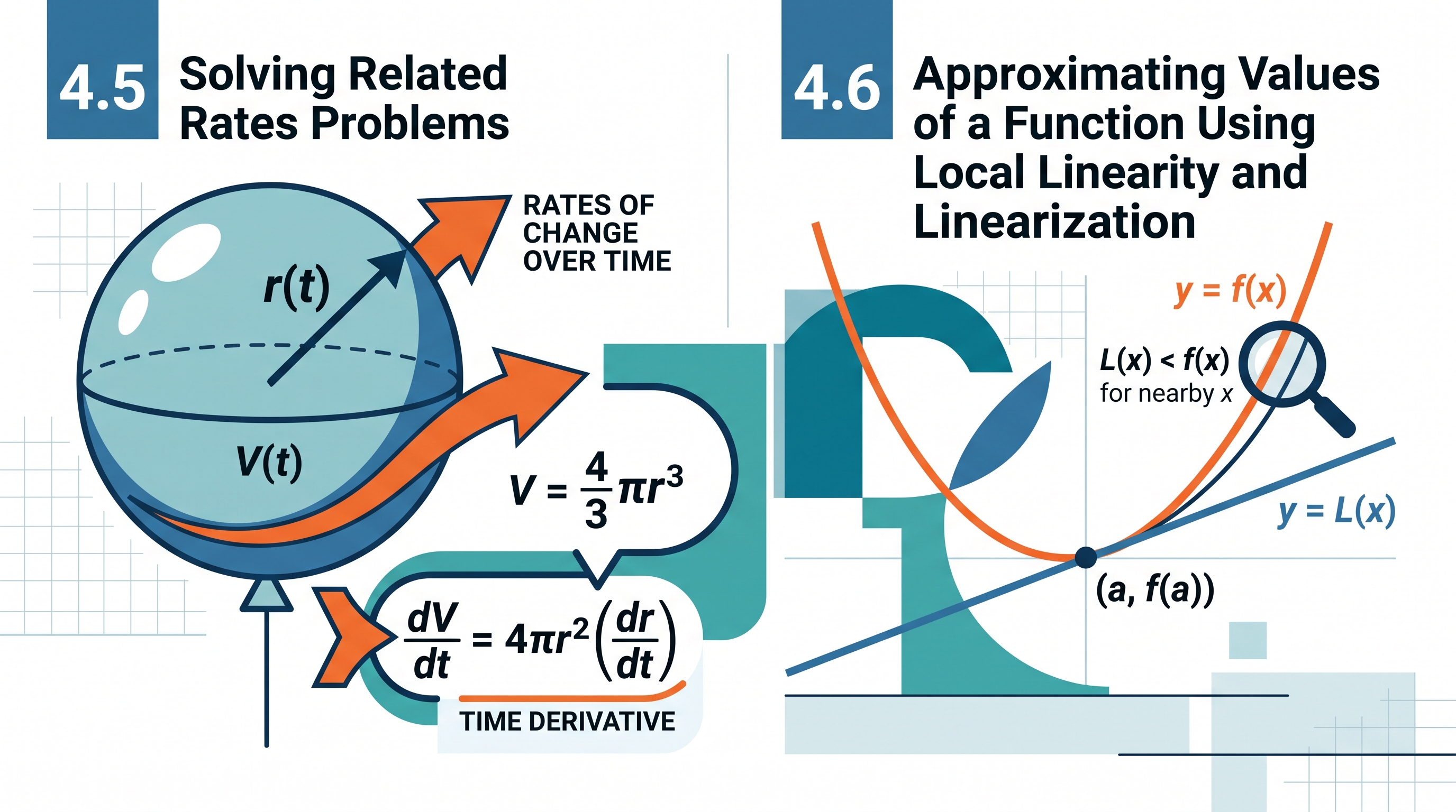
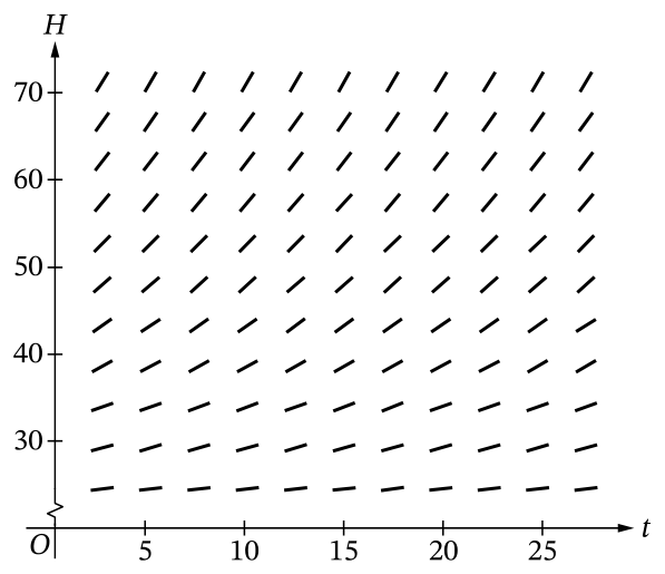
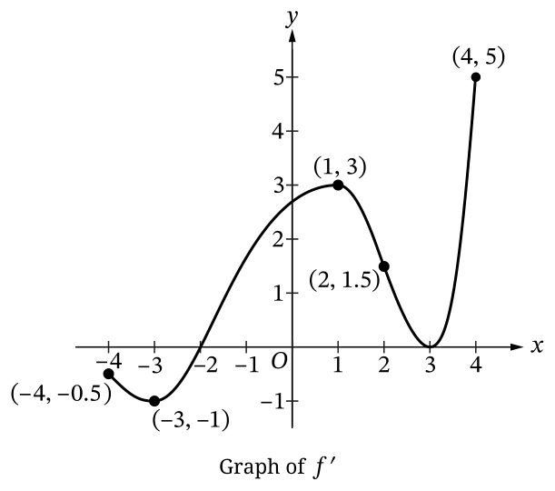
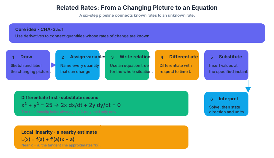
4.6 Approximating Values of a Function Using Local Linearity and Linearization
Key concepts: Tangent-line approximation · Local linearity · Linearization · Taylor-polynomial representation for approximating values near x = a (BC only)
How to build the tangent-line approximation L(x) = f(a) + f'(a)(x - a), use it to estimate values such as the square root of 6, and use concavity to tell over- from underestimates.
4.6 Approximating Values of a Function Using Local Linearity and Linearization
Close to a point where you know a function's value and its slope, the function behaves almost like its tangent line. That makes the tangent line a practical tool: it turns a hard value such as $\sqrt{6}$ into simple arithmetic, and the shape of the graph tells you whether the estimate is too high or too low.
Local linearity: a curve becomes almost straight nearby
Near a point $x=a$, a smooth curve resembles its tangent line. The tangent line is therefore a locally linear approximation: a line that models the function accurately for inputs close to $a$. This is CHA-3.F.1 and supports Suggested Skill 1.F: Approximate values of a function using the equation of a tangent line.
If $f(a)$ and $f'(a)$ are known, the tangent line at $x=a$ is
$$ L(x)=f(a)+f'(a)(x-a). $$
The approximation is
$$ f(x)\approx L(x) $$
when $x$ is near $a$. The expression $L(x)$ is called the linearization of $f$ at $x=a$.
Worked example: estimating $\sqrt{6}$
Choose the nearby function $f(x)=\sqrt{x}$ and the convenient known point $a=4$, because $f(4)=2$. Since
$$ f'(x)=\frac{1}{2\sqrt{x}}, $$
we have
$$ f'(4)=\frac14. $$
Thus the linearization is
$$ L(x)=2+\frac14(x-4). $$
At $x=6$,
$$ \sqrt{6}\approx L(6) =2+\frac14(2) =2.5. $$
The actual value is approximately $2.449$, so this tangent-line estimate is an overestimate. That comparison is not an accident: $f(x)=\sqrt{x}$ is concave down near $x=4$, and a tangent line lies above a concave-down curve. In general, CHA-3.F.2 connects nearby concavity to approximation error: concave-up behavior produces a tangent-line underestimate, while concave-down behavior produces a tangent-line overestimate.
Misconception check — “A tangent line gives the exact value.”
The tangent line agrees exactly with the function at the point of tangency, $x=a$. Away from $a$, it gives an approximation whose accuracy depends on how close $x$ is to $a$ and how much the graph bends.
Retrieval check
A sphere has radius $r(t)$ and volume $V(t)=\frac43\pi r^3$. If $\frac{dr}{dt}$ is known, differentiate with respect to $t$ before inserting the current radius. For linearization, explain why a concave-up function produces a tangent-line underestimate: the graph bends upward and lies above its tangent line near the point of tangency.
4.7 Using L’Hospital’s Rule for Determining Limits of Indeterminate Forms
Key concepts: L’Hospital’s Rule · Limits of indeterminate forms · The indeterminate form 0/0 · The indeterminate form ∞/∞ · Verifying an indeterminate form before applying L’Hospital’s Rule · Determining limits of functions that produce indeterminate forms · Indeterminate-form labels represent a limiting state, not a value · AP Calculus AB and BC scope for L’Hospital’s Rule
A quotient such as $\dfrac{0}{0}$ does not equal zero, and $\dfrac{\infty}{\infty}$ is not a numerical fraction. These symbols label an indeterminate form: direct substitution has not revealed the limit, because different functions with the same apparent form can approach different values.
4.7 Using L’Hospital’s Rule for Determining Limits of Indeterminate Forms
A quotient such as $\dfrac{0}{0}$ does not equal zero, and $\dfrac{\infty}{\infty}$ is not a numerical fraction. These symbols label an indeterminate form: direct substitution has not revealed the limit, because different functions with the same apparent form can approach different values.
Enduring Understanding — LIM-4: L’Hospital’s Rule allows us to determine the limits of some indeterminate forms.
The learning objective is LIM-4.A: Determine limits of functions that result in indeterminate forms. Essential knowledge LIM-4.A.1 identifies $\dfrac{0}{0}$ and $\dfrac{\infty}{\infty}$ as indeterminate forms. Essential knowledge LIM-4.A.2 connects these forms with L’Hospital’s Rule as a possible method.
First diagnose the form
When ordinary limit laws apply and the denominator approaches a nonzero number, a quotient can be evaluated by dividing the separate limits. But if the denominator approaches zero, that quotient rule cannot be used:
$$ \lim_{x\to a}\frac{f(x)}{g(x)} \neq \frac{\lim_{x\to a}f(x)}{\lim_{x\to a}g(x)} \qquad\text{when}\qquad \lim_{x\to a}g(x)=0. $$
The correct first move is direct substitution, not immediate differentiation.
- Compute the limiting behavior of the numerator.
- Compute the limiting behavior of the denominator.
- Apply L’Hospital’s Rule only if the result is $\dfrac{0}{0}$ or $\dfrac{\infty}{\infty}$.
- Differentiate the numerator and denominator separately.
- Reevaluate the new limit.
For example,
$$ \lim_{x\to 1}\frac{x^2-1}{x-1} $$
produces
$$ \frac{1^2-1}{1-1}=\frac{0}{0}. $$
This does not mean the limit equals $\dfrac{0}{0}$. It means direct substitution is inconclusive. In this particular case, factoring is enough:
$$ \frac{x^2-1}{x-1}
\frac{(x-1)(x+1)}{x-1}
x+1 \qquad (x\ne1), $$
so
$$ \lim_{x\to1}\frac{x^2-1}{x-1}
\lim_{x\to1}(x+1)=2. $$
L’Hospital’s Rule
L’Hospital’s Rule says that, under the appropriate differentiability and existence conditions, if
$$ \lim_{x\to a}f(x)=\lim_{x\to a}g(x)=0 $$
or both functions approach infinity, then
$$ \lim_{x\to a}\frac{f(x)}{g(x)}
\lim_{x\to a}\frac{f'(x)}{g'(x)}, $$
provided the limit on the right exists or approaches infinity in a suitable way.
The rule compares rates of approach. It does not say that a quotient of limits may be replaced mechanically by a quotient of derivatives in every problem. The indeterminate form must be verified first.
The $\dfrac{0}{0}$ form
Consider
$$ \lim_{x\to0}\frac{\sin x}{x}. $$
Direct substitution gives
$$ \frac{\sin 0}{0}=\frac{0}{0}, $$
so L’Hospital’s Rule is eligible:
$$ \lim_{x\to0}\frac{\sin x}{x}
\lim_{x\to0}\frac{\cos x}{1}
\frac{\cos0}{1}
$$
The same limit can be established by other calculus methods; L’Hospital’s Rule is useful because differentiation removes the indeterminate quotient.
The $\dfrac{\infty}{\infty}$ form
Now examine
$$ \lim_{x\to\infty}\frac{3x^2+1}{2x^2-5}. $$
As $x\to\infty$, both the numerator and denominator approach infinity, so the expression has the form $\dfrac{\infty}{\infty}$. Applying the rule gives
$$ \lim_{x\to\infty}\frac{6x}{4x}
\lim_{x\to\infty}\frac{3}{2}
\frac{3}{2}. $$
Here the rule exposes the dominant growth rates of the two functions.
A scope and notation warning
Misconception — “The limit equals $\dfrac{0}{0}$.” Writing
$$ \lim_{x\to a}\frac{f(x)}{g(x)}=\frac{0}{0} $$
is incorrect. Instead write: “Direct substitution gives the indeterminate form $\dfrac{0}{0}$,” and then continue with an appropriate method.
For AP Calculus AB and BC, $\dfrac{0}{0}$ and $\dfrac{\infty}{\infty}$ are recognized as indeterminate forms, but L’Hospital’s Rule is not required as an AP-exam method. Treat it as an enrichment technique unless a particular course or teacher explicitly assesses it. Other forms, including $\infty-\infty$, are outside the assessed AP Calculus AB and BC scope described here.
When L’Hospital’s Rule is used in a setting that permits it, the reasoning must include the diagnosis:
“Because the numerator and denominator both approach $0$, the expression has the indeterminate form $\dfrac{0}{0}$; therefore L’Hospital’s Rule may be applied.”
This explicitly demonstrates Skill 3.D: Use mathematical reasoning to solve problems by checking the condition before executing the procedure.
Retrieval check
For
$$ \lim_{x\to2}\frac{x^2-4}{x^2-3x+2}, $$
direct substitution gives $\dfrac{0}{0}$. Is that the answer? No: it is only a diagnosis. Factoring produces
$$ \frac{(x-2)(x+2)}{(x-2)(x-1)}
\frac{x+2}{x-1}, $$
so the limit is
$$ \boxed{4}. $$
The essential habit is: verify the indeterminate form first, then choose a valid method.
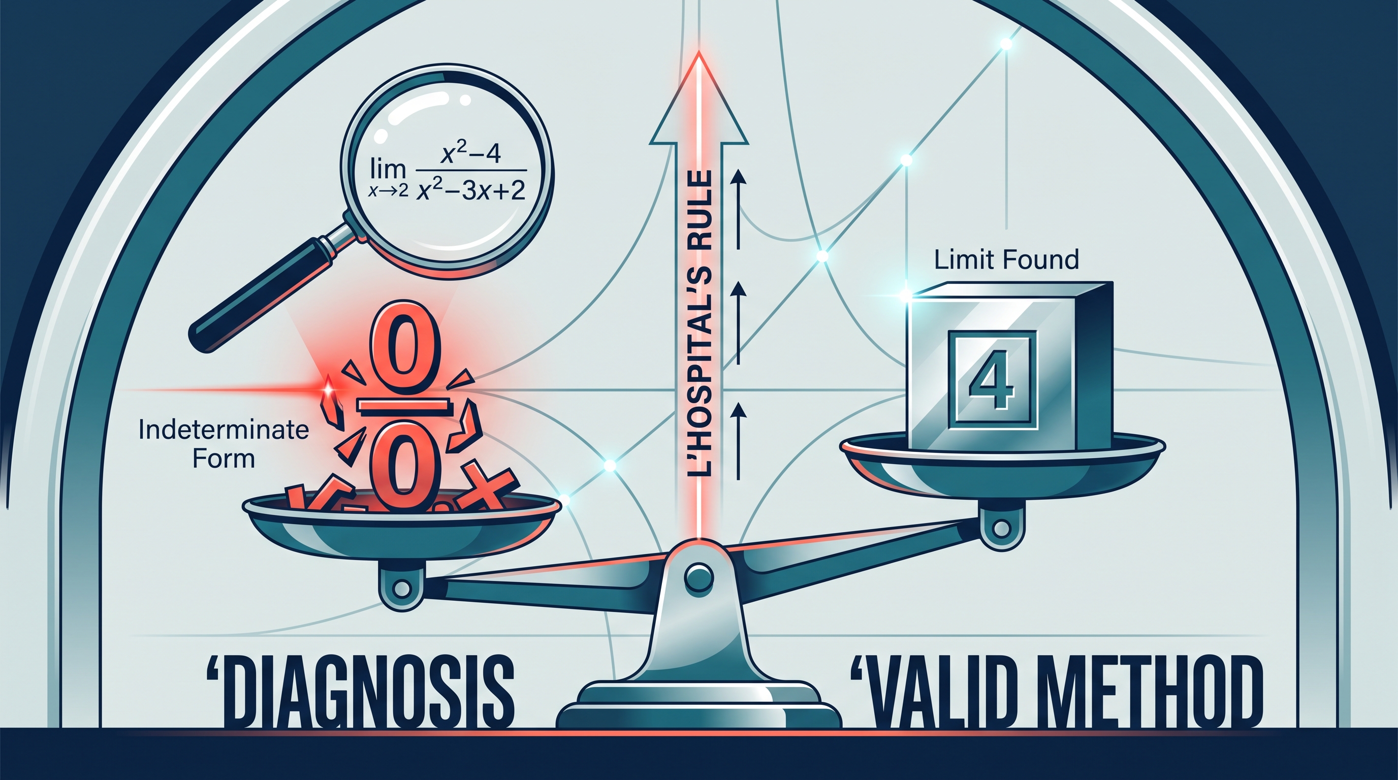
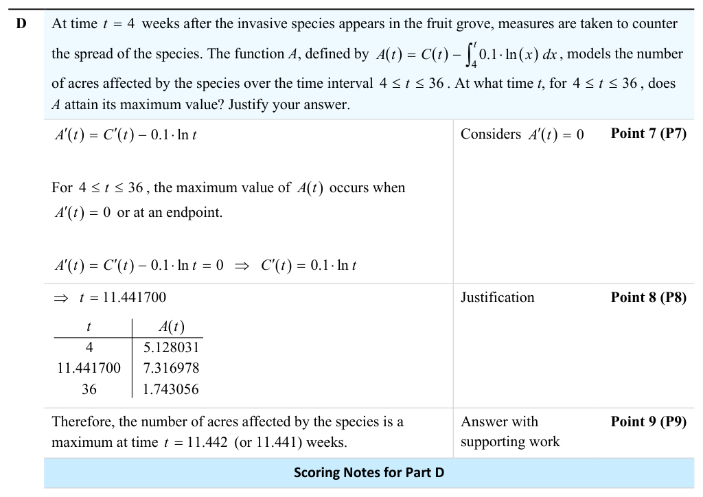
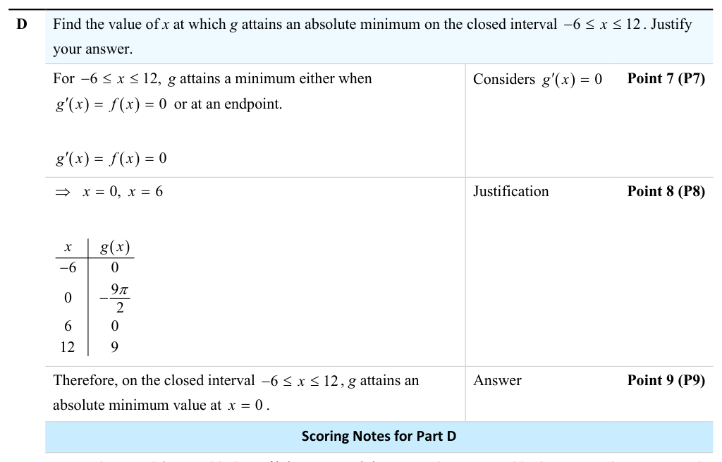
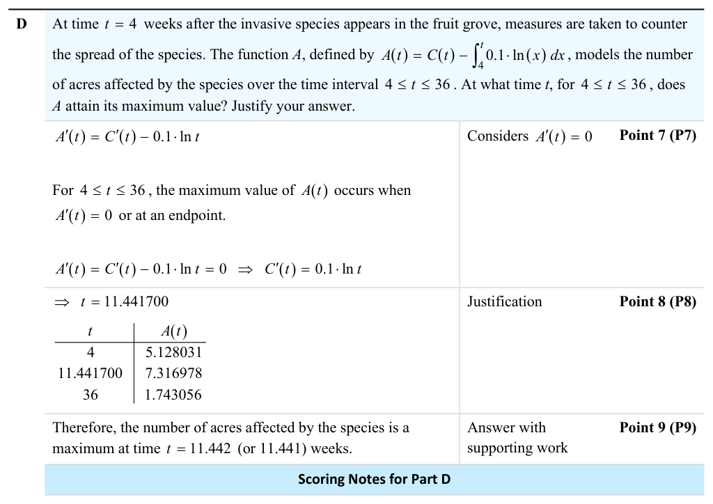
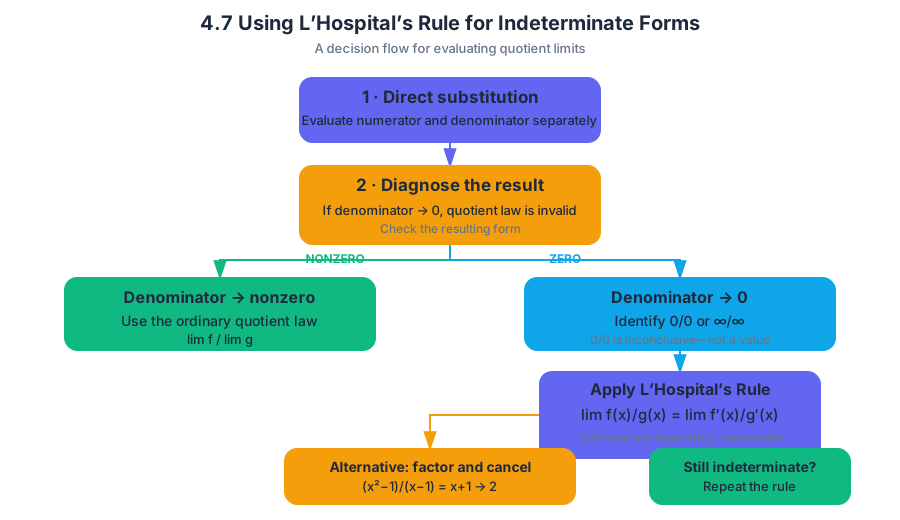
5.1 Using the Mean Value Theorem
Key concepts: Mean Value Theorem and its use in drawing conclusions about function behavior · Continuity on a closed interval · Justifying conclusions with mathematical reasoning · Existence theorems and conclusions about behavior without precisely locating values
How the Mean Value Theorem guarantees a point where the instantaneous rate of change equals the average rate over an interval, and how to justify using it.
5.1 Using the Mean Value Theorem
A function can reveal that something must have happened without telling you exactly where it happened. The Mean Value Theorem proves this for rates of change; the Extreme Value Theorem proves that highest and lowest values exist under the right conditions.
Two existence theorems, two different guarantees
| Theorem | Required conditions | Guaranteed conclusion |
|---|---|---|
| Mean Value Theorem | $f$ is continuous on $[a,b]$ and differentiable on $(a,b)$ | At some $c$ in $(a,b)$, $f'(c)=\dfrac{f(b)-f(a)}{b-a}$ |
| Extreme Value Theorem | $f$ is continuous on the closed interval $[a,b]$ | $f$ has at least one absolute minimum and at least one absolute maximum on $[a,b]$ |
Both are existence theorems: they establish that a value or behavior occurs, but they may not identify its exact location. This distinction matters in applications. A theorem may prove that a driver exceeded a speed limit somewhere on a highway without specifying the precise mile marker.
5.1 The Mean Value Theorem: matching an average rate
The average rate of change of $f$ from $x=a$ to $x=b$ is the slope of the secant line:
$$ \frac{f(b)-f(a)}{b-a}. $$
The Mean Value Theorem says that if $f$ is continuous on $[a,b]$ and differentiable on $(a,b)$, then at least one interior point $c$ satisfies
$$ f'(c)=\frac{f(b)-f(a)}{b-a}. $$
In plain language, the function’s instantaneous rate equals its overall average rate at least once.
Worked contextual example. A driver travels $120$ miles in $2$ hours. Let $s(t)$ denote position, in miles, $t$ hours after departure. The average velocity is
$$ \frac{s(2)-s(0)}{2-0}=\frac{120}{2}=60\text{ miles per hour}. $$
If $s$ is continuous on $[0,2]$ and differentiable on $(0,2)$, the Mean Value Theorem guarantees some time $c$ with
$$ s'(c)=60. $$
If the posted speed limit is $55$ miles per hour, an average of $60$ does not by itself say when the driver went fast, but the Mean Value Theorem guarantees an instant at which the driver’s velocity was exactly $60$ miles per hour, which is enough to conclude that the driver was speeding at that moment.
The assessed reasoning process is 3.E Provide reasons or rationales for solutions and conclusions. A complete justification names the hypotheses—continuity on $[a,b]$ and differentiability on $(a,b)$—then states the theorem’s conclusion and connects it to the context.
Misconception check — “The average rate is the rate at the midpoint.”
The Mean Value Theorem guarantees a point $c$, but not usually $c=\dfrac{a+b}{2}$. The matching point may occur anywhere inside the interval.
Retrieval check. A function $f$ is continuous on $[1,5]$ and differentiable on $(1,5)$, with $f(1)=3$ and $f(5)=11$. What does the Mean Value Theorem guarantee? Answer: at least one $c$ in $(1,5)$ with $f'(c)=\dfrac{11-3}{5-1}=2$. The theorem does not say where $c$ is, and there may be more than one.
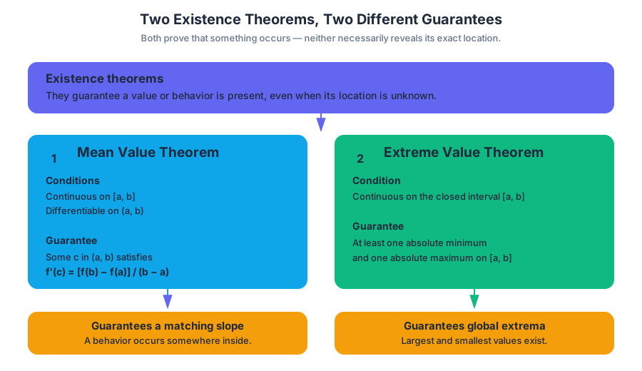
5.2 Extreme Value Theorem, Global Versus Local Extrema, and Critical Points
Key concepts: Extreme Value Theorem · Continuity on a closed interval · Global (absolute) extrema · Local extrema · Critical points · Using the first derivative to identify extrema · Justifying conclusions with mathematical reasoning · Existence theorems and conclusions about behavior without precisely locating values
What the Extreme Value Theorem guarantees, how global and local extrema differ, and how critical points and endpoints locate absolute extrema on a closed interval.
5.2 Extreme Value Theorem, Global Versus Local Extrema, and Critical Points
Topic 5.1's Mean Value Theorem guarantees that a certain rate occurs somewhere, without saying where. The Extreme Value Theorem is the same kind of existence theorem for values: under the right conditions, a function must reach a highest and a lowest value. This page states those conditions, separates global from local extrema, and introduces critical points, the only interior locations where an extremum can occur.
5.2 The Extreme Value Theorem: proving extrema exist
The Extreme Value Theorem (EVT) states:
If a function $f$ is continuous over the closed interval $[a,b]$, then the Extreme Value Theorem guarantees that $f$ has at least one minimum value and at least one maximum value on $[a,b]$.
This is the exact hypothesis in FUN-1.C.1 and the core of learning objective FUN-1.C: Justify conclusions about functions by applying the Extreme Value Theorem. The phrase closed interval is essential: both endpoints must be included.
A function may fail to attain an extreme value if continuity or closedness is missing. For example, $f(x)=\dfrac{1}{x}$ is not continuous on an interval containing $x=0$, and $f(x)=x$ on the open interval $(0,1)$ has neither an attained absolute minimum nor an attained absolute maximum.
Global, local, and critical points
A global (absolute) maximum on a domain is a function value at least as large as every other value in that domain. A global (absolute) minimum is at most every other value. A local (relative) maximum is highest only within a nearby interval, while a local (relative) minimum is lowest nearby.
A critical point occurs at a point in the domain where
$$ f'(x)=0 $$
or where $f'(x)$ does not exist. This definition is FUN-1.C.2. The corresponding $x$-value is often called a critical number.
FUN-1.C.3 states that all local (relative) extrema occur at critical points, although not all critical points are local extrema. For instance, $f(x)=x^3$ has $f'(0)=0$, but the function continues increasing through $x=0$; therefore, $x=0$ is critical but is not a local maximum or minimum.
Sign-change insight: If $f'$ changes from negative to positive at $x=2$, the function changes from decreasing to increasing, so $f$ has a local minimum at $x=2$.
Absolute extrema on a closed interval
To locate an absolute minimum or maximum on $[a,b]$, evaluate $f$ at every relevant interior critical point and at both endpoints. The endpoint check is indispensable: a global extreme can occur where the derivative is not zero because endpoints are not interior points.
Worked example. Find the absolute minimum of
$$ f(x)=x^2-4x+5 $$
on $[0,5]$. First,
$$ f'(x)=2x-4, $$
so the critical point is $x=2$. Compare:
$$ f(0)=5,\qquad f(2)=1,\qquad f(5)=10. $$
Thus the absolute minimum value is
$$ \boxed{1} $$
at $x=2$. The conclusion is justified because the polynomial is continuous on $[0,5]$, so the EVT guarantees that an absolute minimum exists, and the critical-point/endpoints comparison identifies it.
Retrieval check. A function is continuous on $[-3,4]$, and $f'(x)$ is undefined at $x=1$ but defined elsewhere. What points must be checked when searching for an absolute minimum? Answer: $x=-3$, $x=1$, and $x=4$, provided $x=1$ lies in the function’s domain.
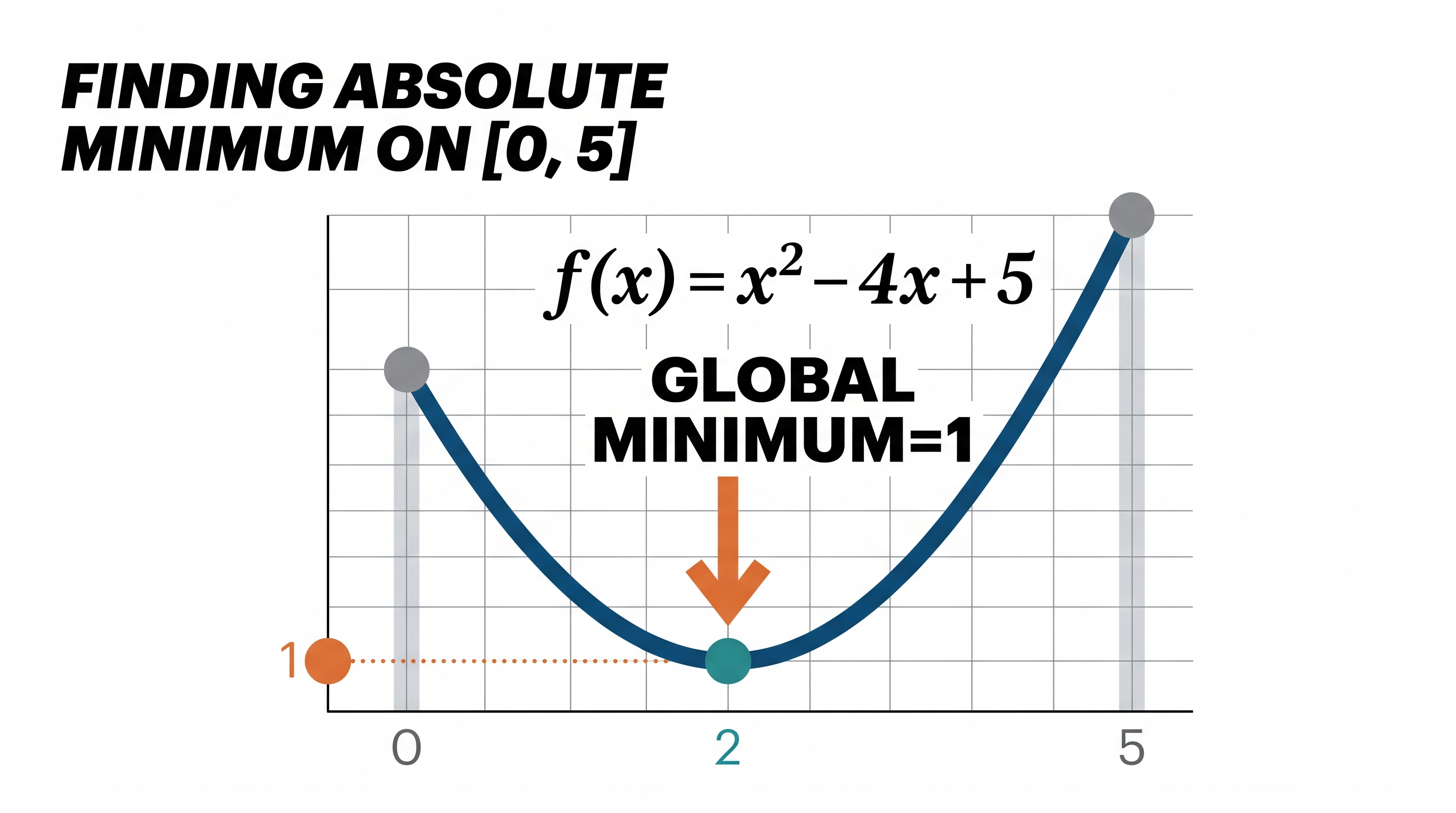
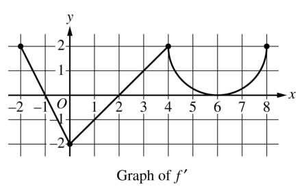
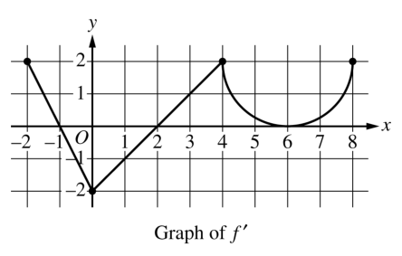
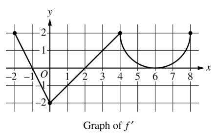
5.3 Determining Intervals on Which a Function Is Increasing or Decreasing
Key concepts: Using the first derivative to determine where a function is increasing or decreasing · Using the sign of f′ on open intervals to analyze function behavior · Justifying conclusions about increasing/decreasing behavior and extrema · Interpreting the graph of f′ to determine the behavior of f · Applying derivative-based reasoning to a specific value, such as x = −3 · Using appropriate mathematical representations and explanations
How to use the sign of the first derivative, and a sign chart built from critical numbers, to find the intervals on which a function is increasing or decreasing.
5.3 Determining Intervals on Which a Function Is Increasing or Decreasing
A derivative can reveal whether a graph is climbing or falling without requiring us to see the graph itself. The essential question is simple: what does the sign of $f'(x)$ say about the behavior of $f(x)$?
The sign of the derivative controls direction
If $f'(x)>0$ throughout an open interval, then $f$ is increasing on that interval. If $f'(x)<0$ throughout an open interval, then $f$ is decreasing there. The derivative acts like a slope meter: positive slopes push the graph upward as $x$ increases, while negative slopes pull it downward.
Derivative sign rule
$$f'(x)>0 \Longrightarrow f \text{ is increasing}$$
$$f'(x)<0 \Longrightarrow f \text{ is decreasing}$$
The word throughout matters. To justify that $f$ is increasing on $(a,b)$, you must establish that $f'(x)>0$ for every $x$ in $(a,b)$, not merely calculate one positive derivative value.
From a derivative formula to intervals
Use the critical numbers identified earlier—where $f'(c)=0$ or does not exist—to divide the domain into intervals for a sign chart. Then determine the sign of $f'$ on each interval. One convenient test value is enough when the sign cannot change inside that interval, but the conclusion must refer to the entire interval.
Consider
$$f'(x)=5+3x.$$
Set the derivative equal to zero:
$$5+3x=0 \quad\Longrightarrow\quad x=-\frac{5}{3}.$$
This divides the real line into
$$\left(-\infty,-\frac{5}{3}\right) \quad\text{and}\quad \left(-\frac{5}{3},\infty\right).$$
Choose one test value from each interval:
| Interval | Test value | Sign of $f'(x)=5+3x$ | Behavior of $f$ |
|---|---|---|---|
| $\left(-\infty,-\frac{5}{3}\right)$ | $x=-3$ | $5+3(-3)=-4<0$ | Decreasing |
| $\left(-\frac{5}{3},\infty\right)$ | $x=0$ | $5+3(0)=5>0$ | Increasing |
Therefore, $f$ is decreasing on $\left(-\infty,-\frac{5}{3}\right)$ because $f'(x)<0$ there, and increasing on $\left(-\frac{5}{3},\infty\right)$ because $f'(x)>0$ there. Notice how evaluating at $x=-3$ is not the final conclusion; it supplies evidence for the sign on the whole interval containing $-3$.
Worked contextual example
Suppose $P(t)$ represents the population of a microorganism colony, and its derivative satisfies
$$P'(t)=(t-2)(t-5), \qquad 0\le t\le 7.$$
The critical numbers in the domain are $t=2$ and $t=5$. Test one value in each resulting interval:
| Time interval | Test value | Sign of $P'(t)$ | Population behavior |
|---|---|---|---|
| $(0,2)$ | $t=1$ | $(1-2)(1-5)>0$ | Increasing |
| $(2,5)$ | $t=3$ | $(3-2)(3-5)<0$ | Decreasing |
| $(5,7)$ | $t=6$ | $(6-2)(6-5)>0$ | Increasing |
Therefore, $P$ increases on $(0,2)$, decreases on $(2,5)$, and increases on $(5,7)$. At $t=2$, the sign changes from positive to negative, so the colony has a relative maximum. At $t=5$, the sign changes from negative to positive, so the colony has a relative minimum.
The interval conclusions are this topic's work. The sign changes at $t=2$ and $t=5$ are what Topic 5.4's First Derivative Test reads to classify those points as relative extrema.
These conclusions demonstrate FUN-4.A: Justify conclusions about the behavior of a function based on the behavior of its derivatives: the first derivative shows the intervals on which a function is increasing or decreasing. A complete justification gives the sign of $f'$ on the whole interval as the reason, not merely the answer.
Retrieval check: Suppose $f'(x)=(x-1)(x+4)$. Which critical numbers divide the real line, and on which intervals is $f$ increasing? Explain using the sign of $f'$. (Here $f'>0$ on $(-\infty,-4)$ and on $(1,\infty)$, so $f$ is increasing there; $f'<0$ on $(-4,1)$, so $f$ is decreasing there.)
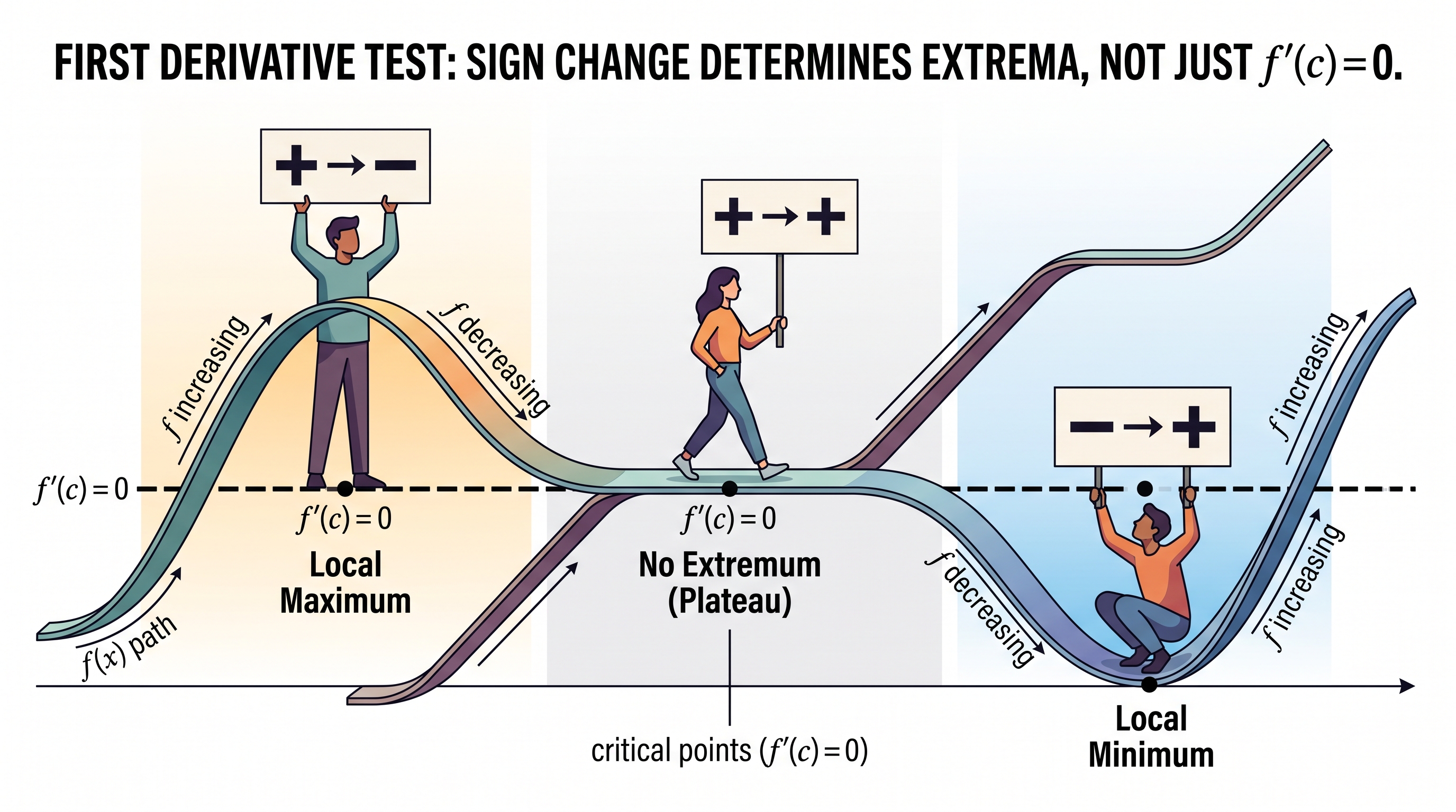
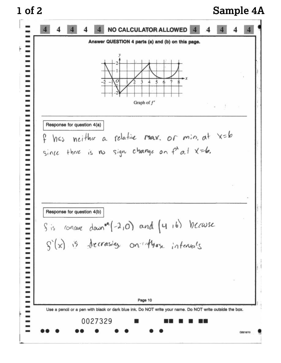
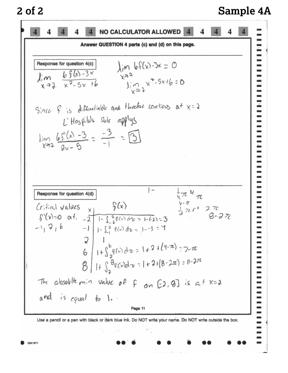
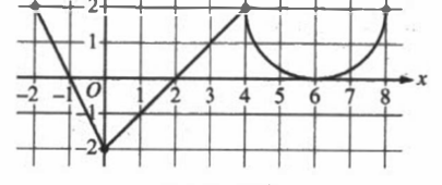
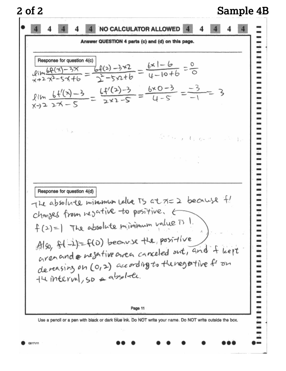
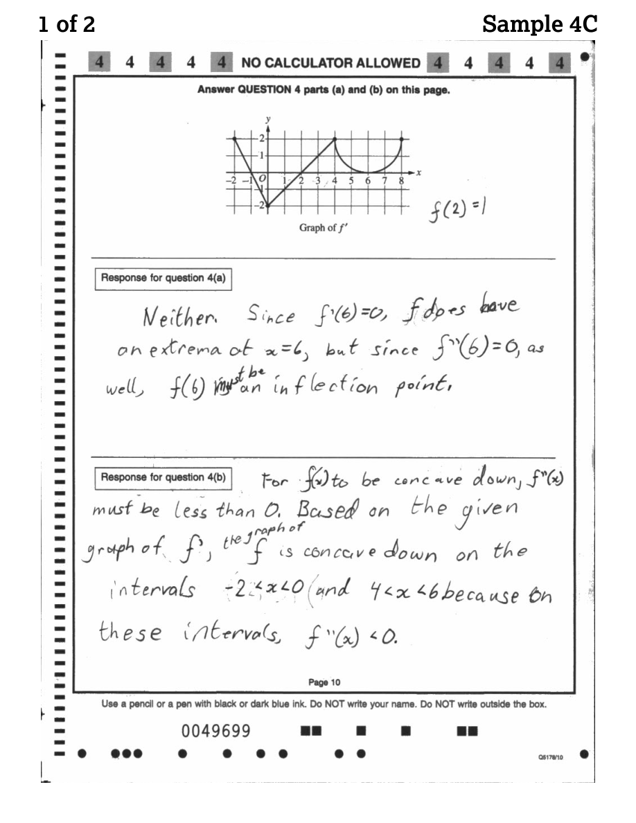
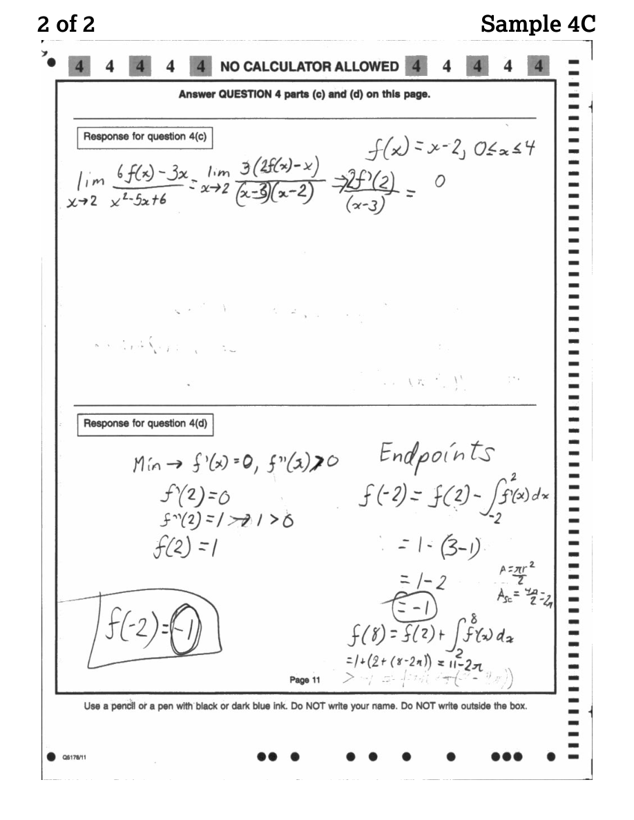
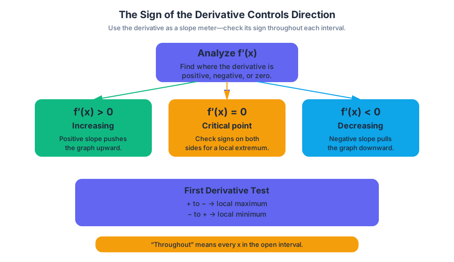
5.4 Using the First Derivative Test to Determine Relative (Local) Extrema
Key concepts: Critical points and their role in locating relative (local) extrema · The First Derivative Test for relative (local) maxima and minima · Determining extrema from a graph or sign chart of the derivative · Justifying conclusions about increasing/decreasing behavior and extrema · Interpreting the graph of f′ to determine the behavior of f · The relationship between continuity, critical points, and relative extrema · Using appropriate mathematical representations and explanations
How the First Derivative Test uses a sign change in the first derivative at a critical number to identify relative maxima and minima.
5.4 Using the First Derivative Test to Determine Relative (Local) Extrema
Topic 5.3 used the sign of $f'$ to find where a function rises and where it falls. A relative extremum is a place where that direction reverses, so the same sign chart can also locate local maxima and minima. This page turns that observation into the First Derivative Test.
The First Derivative Test
A relative, or local, extremum occurs when the function changes direction near a point. The First Derivative Test detects that direction change by comparing the signs of $f'$ on the two sides of a critical number.
First Derivative Test
- If $f'$ changes from positive to negative at $x=c$, then $f$ changes from increasing to decreasing and has a relative maximum at $x=c$.
- If $f'$ changes from negative to positive at $x=c$, then $f$ changes from decreasing to increasing and has a relative minimum at $x=c$.
- If $f'$ does not change sign at $x=c$, the test does not identify a relative extremum there.
For example, suppose a derivative sign chart is
$$ \begin{array}{c|ccc} x & (-\infty,2) & 2 & (2,\infty)\ \hline f'(x) & + & 0 & - \end{array} $$
The function increases before $x=2$ and decreases afterward. Thus $f$ has a relative maximum at $x=2$.
By contrast,
$$ \begin{array}{c|ccc} x & (-\infty,6) & 6 & (6,\infty)\ \hline f'(x) & + & 0 & + \end{array} $$
shows that $f$ increases on both sides of $x=6$. The derivative is zero at $x=6$, but there is no relative extremum because the function never changes direction.
Worked contextual example
Suppose $P(t)$ represents the population of a microorganism colony, and its derivative satisfies
$$P'(t)=(t-2)(t-5), \qquad 0\le t\le 7.$$
The critical numbers in the domain are $t=2$ and $t=5$. Test one value in each resulting interval:
| Time interval | Test value | Sign of $P'(t)$ | Population behavior |
|---|---|---|---|
| $(0,2)$ | $t=1$ | $(1-2)(1-5)>0$ | Increasing |
| $(2,5)$ | $t=3$ | $(3-2)(3-5)<0$ | Decreasing |
| $(5,7)$ | $t=6$ | $(6-2)(6-5)>0$ | Increasing |
Therefore, $P$ increases on $(0,2)$, decreases on $(2,5)$, and increases on $(5,7)$. At $t=2$, the sign changes from positive to negative, so the colony has a relative maximum. At $t=5$, the sign changes from negative to positive, so the colony has a relative minimum.
Misconception check: $f'(c)=0$ is not enough
A common error is to state, “$f'(c)=0$, so $f$ has a maximum or minimum at $c$.” Zero derivative only identifies a point that requires investigation. The decisive evidence is the sign change: positive-to-negative gives a local maximum, negative-to-positive gives a local minimum, and no sign change gives neither by the First Derivative Test.
These conclusions demonstrate FUN-4.A: Justify conclusions about the behavior of a function based on the behavior of its derivatives, using FUN-4.A.2: The first derivative of a function can determine the location of relative (local) extrema of the function. They also rely on FUN 2: Connecting Representations, when a formula, graph, or sign chart for $f'$ is translated into behavior of $f$, and FUN 3: Justification, when the sign information is stated as a reason rather than merely an answer.
Retrieval check: If $f'(x)<0$ on $(1,4)$ and $f'(x)>0$ on $(4,7)$, what occurs at $x=4$? Explain using both the behavior of $f$ and the sign change in $f'$.
5.5 Using the Candidates Test to Determine Absolute (Global) Extrema
Key concepts: Candidates Test for determining absolute (global) extrema · Critical points · Endpoints of a closed interval · Absolute extrema on a closed interval · Using derivatives to determine function behavior · Applying mathematical definitions, theorems, and tests · Justifying conclusions about extrema and concavity
How the Candidates Test finds absolute extrema on a closed interval by comparing function values at interior critical points and at both endpoints.
5.5 Using the Candidates Test to Determine Absolute (Global) Extrema
An absolute maximum is the greatest value a function reaches on a specified domain, while an absolute minimum is the least value it reaches. On a closed interval, these global extrema can occur only at two kinds of locations: critical points inside the interval and the endpoints.
FUN-4.A.3: Absolute (global) extrema of a function on a closed interval can only occur at critical points or at endpoints.
The word candidate matters: a critical point or endpoint is not automatically a maximum or minimum. It is simply a location that must be tested. The Candidates Test turns that idea into a finite comparison.
The Candidates Test on a closed interval
For a function $f$ that is continuous on the closed interval $[a,b]$, use this procedure:
- Find all critical points in $(a,b)$: values of $x$ where $f'(x)=0$ or where $f'(x)$ does not exist.
- Keep only the critical points that lie in the interval.
- Evaluate $f$ at every critical point and at both endpoints, $x=a$ and $x=b$.
- Compare the resulting function values.
The largest value is the absolute maximum, and the smallest value is the absolute minimum. The theorem behind the procedure is the Extreme Value Theorem: continuity on a closed interval guarantees that absolute extrema exist, and the Candidates Test identifies where they can occur.
Worked example: comparing every candidate
Let
$$ f(x)=x^3-3x^2+1 $$
on $[-1,3]$. First differentiate:
$$ f'(x)=3x^2-6x=3x(x-2). $$
Thus the critical points are $x=0$ and $x=2$, both inside $[-1,3]$. Now evaluate all candidates:
$$ \begin{aligned} f(-1)&=-3,\ f(0)&=1,\ f(2)&=-3,\ f(3)&=1. \end{aligned} $$
The absolute maximum value is $1$, occurring at $x=0$ and $x=3$. The absolute minimum value is $-3$, occurring at $x=-1$ and $x=2$. A complete written justification is: “Because $f$ is continuous on $[-1,3]$, its absolute extrema occur at critical points or endpoints. Comparing $f(-1)$, $f(0)$, $f(2)$, and $f(3)$ gives an absolute maximum of $1$ and an absolute minimum of $-3$.”
Misconception check — “The critical point is the answer.” A critical point is only a candidate. In the example, $x=0$ is a critical point and gives the absolute maximum, but $x=2$ is also critical and gives the absolute minimum. The endpoints are equally important: $x=-1$ ties for the minimum, and $x=3$ ties for the maximum.
What changes on an open interval?
The Candidates Test above is specifically a closed-interval method. If the domain is $(a,b)$, the endpoints are not included and cannot be locations where the function attains an absolute extremum. Likewise, if the function is not continuous on $[a,b]$, the Extreme Value Theorem does not apply automatically, so the required justification must address the actual domain and behavior.
Suggested skill 1.E — Apply appropriate mathematical rules or procedures, with and without technology is explicit for Topic 5.5. A calculator may help locate zeros of $f'(x)$ or evaluate complicated expressions, but the mathematical procedure still requires identifying the interval, checking domain membership, evaluating every candidate, and comparing values. A calculator list of values without that structure is not a justification.
Retrieval check. A function $f$ is continuous on $[0,6]$, and its only critical points are $x=2$ and $x=5$. Which values must be compared to find its absolute extrema, and why is $f'(2)=0$ not enough to call $f(2)$ the absolute maximum? Answer: compare $f(0)$, $f(2)$, $f(5)$, and $f(6)$; a critical point is only a candidate until every candidate value has been compared.
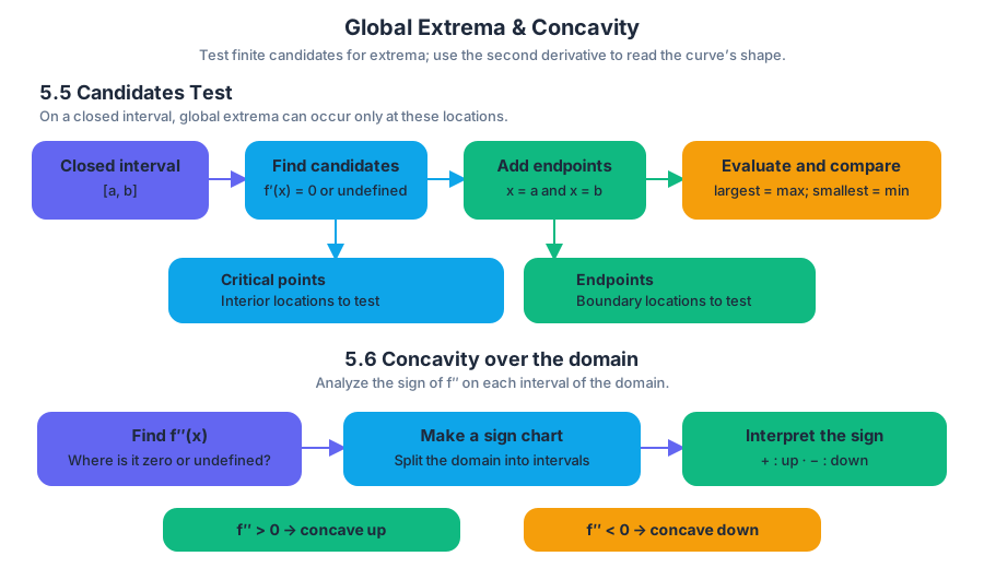
5.6 Determining Concavity of Functions over Their Domains
Key concepts: Concavity of functions · Intervals of upward concavity · Intervals of downward concavity · Using derivatives to determine function behavior · Applying mathematical definitions, theorems, and tests · Justifying conclusions about extrema and concavity
How the sign of the second derivative determines the intervals on which a function is concave upward or concave downward.
5.6 Determining Concavity of Functions over Their Domains
Two graphs can both be rising and still look nothing alike: one bends upward and climbs ever faster, while the other bends downward and levels off. Concavity names that bend. This page shows how the sign of $f''$ identifies it on each interval of a function's domain.
A graph’s first derivative tells whether the function is rising or falling; its second derivative tells how that rise or fall is changing. This is the difference between a road climbing at a steady grade and a road whose grade is becoming steeper.
FUN-4: A function’s derivative can be used to understand some behaviors of the function.
FUN-4.A: Justify conclusions about the behavior of a function based on the behavior of its derivatives.
FUN-4.B: Determine intervals on which a function is concave upward or downward.
FUN-4.B.1: The second derivative of a function provides information about the behavior of the first derivative.
A function is concave upward on an interval when its slopes are increasing from left to right. A function is concave downward when its slopes are decreasing from left to right. When the second derivative exists, the standard test is:
$$ f''(x)>0 \quad \Longrightarrow \quad f\text{ is concave upward}, $$
$$ f''(x)<0 \quad \Longrightarrow \quad f\text{ is concave downward}. $$
Finding intervals of concavity
To determine concavity over the domain, find $f''(x)$, locate values where $f''(x)=0$ or $f''(x)$ does not exist, and use those values to divide the domain into intervals. Then determine the sign of $f''$ on each interval and state the conclusion in words.
Worked example: a concavity sign chart
For
$$ g(x)=x^3-6x^2+4, $$
we have
$$ g'(x)=3x^2-12x \qquad\text{and}\qquad g''(x)=6x-12=6(x-2). $$
The possible concavity boundary is $x=2$. Testing the intervals:
$$ \begin{array}{c|c|c} \text{Interval} & \text{Sign of }g''(x) & \text{Concavity}\ \hline (-\infty,2) & g''(x)<0 & \text{concave downward}\ (2,\infty) & g''(x)>0 & \text{concave upward} \end{array} $$
A precise justification is: “Since $g''(x)=6(x-2)$ is negative for $x<2$, $g$ is concave downward on $(-\infty,2)$. Since $g''(x)$ is positive for $x>2$, $g$ is concave upward on $(2,\infty)$.” The value $x=2$ separates intervals; it is not itself an interval of concavity.
Misconception check — “$f''(x)=0$ means there is an inflection point.” It does not. The sign of $f''$ must change across the value. Here, $g''$ changes from negative to positive at $x=2$, so the graph changes from downward to upward concavity. Merely solving $f''(x)=0$ is not enough.
Retrieval check
For absolute extrema of a continuous function on $[a,b]$, which values must be compared? For concavity, what must happen to the sign of $f''$ before claiming a change in concavity? Answer: compare the function at every critical point in $(a,b)$ and at both endpoints; a concavity change requires the sign of $f''$ to change across the boundary value.
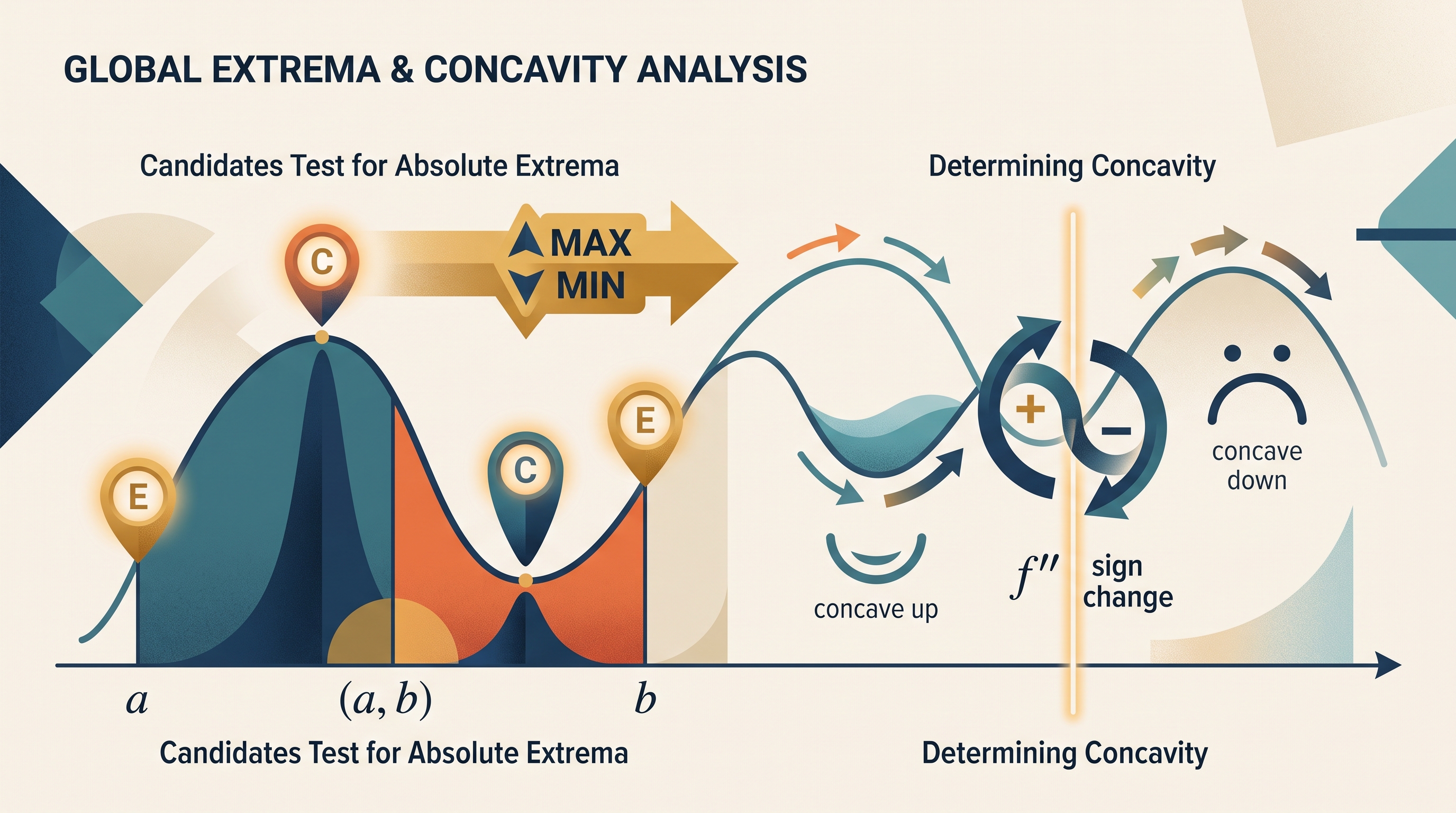
5.7 Using the Second Derivative Test to Determine Extrema
Key concepts: Relative (local) extrema · Second and higher-order derivatives · Parametric, polar, and vector-valued functions
How the Second Derivative Test uses the sign of the second derivative at a critical point to classify it as a relative maximum or minimum, and when the test is inconclusive.
5.7 Using the Second Derivative Test to Determine Extrema
A graph can reveal a local maximum or minimum before any calculation does: near a hilltop, slopes change from positive to negative; near a valley, they change from negative to positive. The Second Derivative Test detects that change in shape by examining $f''$, the derivative of $f'$.
The Second Derivative Test
Let $c$ be a critical point where $f'(c)=0$. If $f''$ exists near $c$, then:
If $f''(c)>0$, $f$ has a relative (local) minimum at $x=c$.
If $f''(c)<0$, $f$ has a relative (local) maximum at $x=c$.
If $f''(c)=0$, the test is inconclusive.
The test works because $f''$ describes how the slope $f'$ is changing. A positive value means the slopes are increasing, as they do while the graph bends upward into a valley. A negative value means the slopes are decreasing, as they do while the graph bends downward over a hill.
Worked example. Consider $f(x)=x^3-3x$. Differentiate:
$$ f'(x)=3x^2-3=3(x-1)(x+1). $$
The critical points are $x=-1$ and $x=1$. Differentiating again gives
$$ f''(x)=6x. $$
Now classify each point:
$$ f''(-1)=-6<0, $$
so $f$ has a relative maximum at $x=-1$. Also,
$$ f''(1)=6>0, $$
so $f$ has a relative minimum at $x=1$. Their coordinates are
$$ f(-1)=2 \qquad\text{and}\qquad f(1)=-2. $$
The test identifies relative extrema: behavior compared with nearby points. It does not by itself prove that the maximum value $2$ or minimum value $-2$ is global over the entire domain. That broader conclusion requires comparing all relevant candidates, including endpoints when an interval is specified.
Second and higher-order derivatives
Differentiating $f'$ produces the second derivative:
$$ f''(x)=\frac{d}{dx}\bigl(f'(x)\bigr) =\frac{d^2f}{dx^2}. $$
Further differentiation produces higher-order derivatives:
$$ f'''(x)=\frac{d}{dx}\bigl(f''(x)\bigr), \qquad f^{(4)}(x)=\frac{d}{dx}\bigl(f'''(x)\bigr), $$
and, in general,
$$ f^{(n)}(x)=\frac{d^n f}{dx^n}. $$
For example, if $f(x)=x^4$, then
$$ f'(x)=4x^3,\qquad f''(x)=12x^2,\qquad f'''(x)=24x,\qquad f^{(4)}(x)=24. $$
The Second Derivative Test specifically uses $f''$. Higher derivatives can describe additional behavior, but they are not automatically part of this test.
Misconception check — “$f''(c)=0$ means there is no extremum.”
False. It means only that the Second Derivative Test cannot decide. For $f(x)=x^4$, $f'(0)=0$ and $f''(0)=0$, yet $x=0$ is a relative minimum.
In the course framework, Topic 5.7 is tagged FUN-4.A.7 for the Second Derivative Test and FUN-4.A.8 for relating relative extrema to absolute extrema. The reasoning is Mathematical Practice 3: Justification, especially 3.D, applying an appropriate test: a complete response states that $f'(c)=0$, gives the sign of $f''(c)$, and only then names the extremum, rather than merely labeling the point.
Retrieval check. Suppose $f'(2)=0$ and $f''(2)<0$. What kind of extremum occurs at $x=2$, and which graph feature of $f'$ supports your answer? A relative maximum occurs because $f'$ is decreasing through zero, changing from positive to negative. AP Calculus BC extends these same ideas to parametrically defined curves, polar curves, and vector-valued functions.
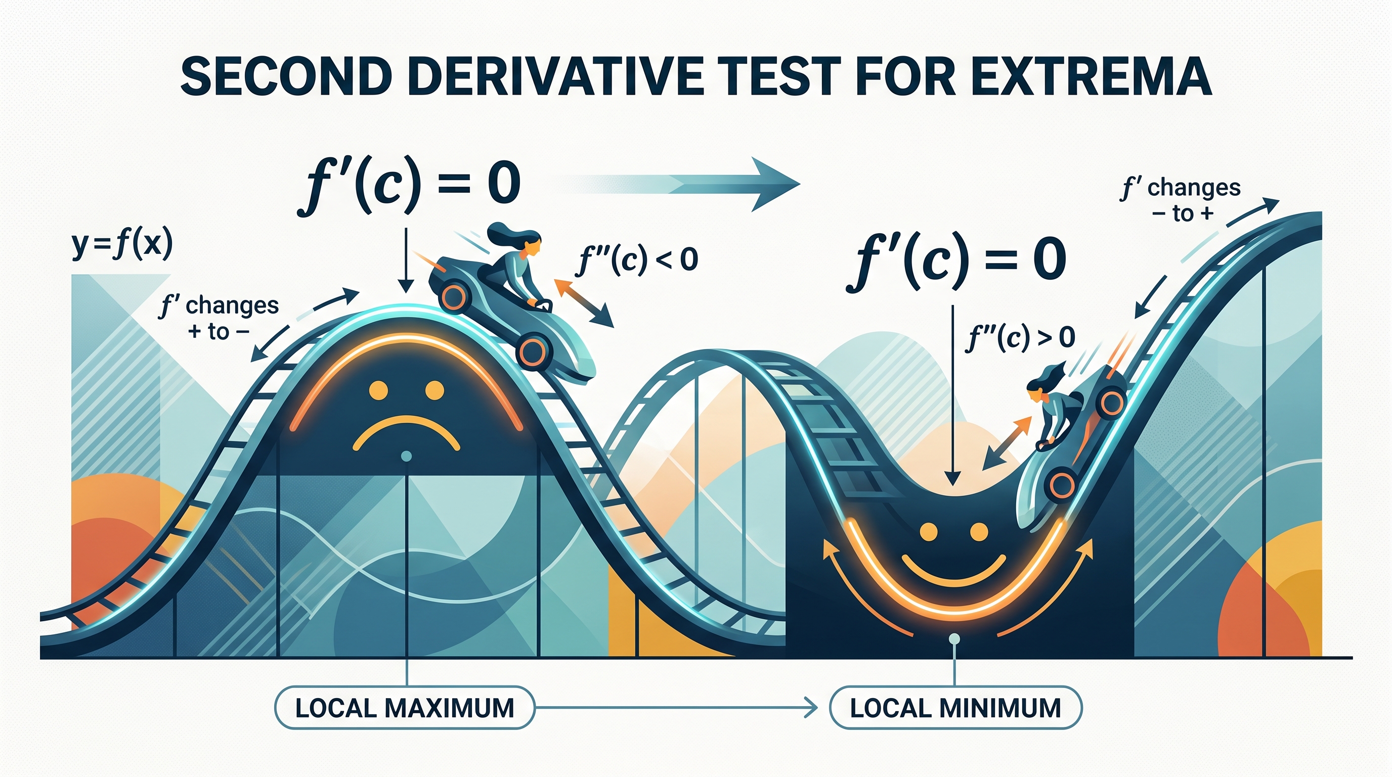
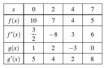
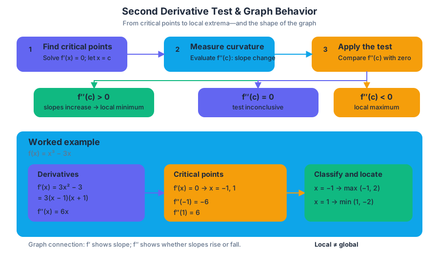
5.8 Sketching Graphs of Functions and Their Derivatives
Key concepts: Graphs of functions and their derivatives · Representing functions with graphs, tables, and verbal expressions · Derivative rules for familiar functions · Product rule for differentiable functions · Quotient rule for differentiable functions · Derivatives of trigonometric functions · Derivatives of inverse functions
How to connect graphs, tables and sign information for a function and its first and second derivatives in order to sketch and explain the function's behavior.
5.8 Sketching Graphs of Functions and Their Derivatives
Every test in this unit links a feature of $f'$ or $f''$ to a feature of $f$. Sketching uses those links in both directions: derivative information produces a graph of $f$, and a graph of $f'$ describes $f$. Every sketch depends on correct derivatives, so this page starts with the differentiation rules.
Derivative rules that support the analysis
Accurate graph analysis depends on selecting the correct derivative rule. Familiar derivatives include
$$ \frac{d}{dx}(\sin x)=\cos x,\qquad \frac{d}{dx}(\cos x)=-\sin x,\qquad \frac{d}{dx}(e^x)=e^x. $$
For a product of differentiable functions,
$$ \frac{d}{dx}\bigl[f(x)g(x)\bigr] =f'(x)g(x)+f(x)g'(x). $$
For a quotient,
$$ \frac{d}{dx}\left(\frac{f(x)}{g(x)}\right)
\frac{g(x)f'(x)-f(x)g'(x)}{[g(x)]^2}, \qquad g(x)\ne 0. $$
The reciprocal identities make trigonometric derivatives manageable:
$$ \tan x=\frac{\sin x}{\cos x},\qquad \cot x=\frac{\cos x}{\sin x},\qquad \sec x=\frac{1}{\cos x},\qquad \csc x=\frac{1}{\sin x}. $$
They lead to
$$ (\tan x)'=\sec^2x,\qquad (\cot x)'=-\csc^2x, $$
$$ (\sec x)'=\sec x\tan x,\qquad (\csc x)'=-\csc x\cot x. $$
For instance, with $h(x)=x^2e^x$,
$$ h'(x)=2xe^x+x^2e^x=e^x(x^2+2x). $$
The first term differentiates the polynomial factor; the second differentiates the exponential factor.
Sketching a function and its derivatives
A reliable sketch combines several representations: a verbal description, a table of values, a graph of $f$, and graphs or sign information for $f'$ and $f''$. Technology can check a table or graph, but it does not replace explaining what the signs mean.
| Information | Meaning for the graph of $f$ |
|---|---|
| $f'(x)>0$ | $f$ is increasing |
| $f'(x)<0$ | $f$ is decreasing |
| $f'(x)=0$ | Horizontal tangent or possible extremum |
| $f''(x)>0$ | Slopes increase; graph bends upward |
| $f''(x)<0$ | Slopes decrease; graph bends downward |
The same table lets you read a graph of $f'$ directly. Where the graph of $f'$ lies above the $x$-axis, $f$ is increasing; where it lies below, $f$ is decreasing. Where $f'$ crosses the axis, $f$ has a relative extremum. Where the graph of $f'$ is rising, $f''>0$ and $f$ bends upward; where it is falling, $f$ bends downward. A turning point of $f'$ therefore marks an inflection point of $f$.
For $f(x)=x^3-3x$, the derivative graph $y=f'(x)=3x^2-3$ is an upward-opening parabola. Its zeros at $x=-1$ and $x=1$ are the horizontal tangencies of $f$; the sign pattern of $f'$ gives increasing, decreasing, and increasing intervals, while $f''(x)=6x$ identifies the local maximum and minimum through the Second Derivative Test.
This multirepresentational reasoning is Mathematical Practice 2: Connecting Representations and is assessed through FUN 2. Justification is Mathematical Practice 3: Justification, especially 3.D, when the response must explain why a point is a maximum or minimum rather than merely label it. Topic 5.7 is tagged FUN-4.A.7 for the Second Derivative Test and FUN-4.A.8 for distinguishing relative from absolute extrema.
Retrieval check. For $f(x)=x^3-3x$, the graph of $f'(x)=3x^2-3$ has its vertex at $x=0$. What does that vertex say about the graph of $f$? It marks an inflection point: $f'$ changes from decreasing to increasing there, so $f$ changes from bending downward to bending upward.
5.9 Connecting a Function, Its First Derivative, and Its Second Derivative
Key concepts: Higher-order derivatives · Connecting a function, its first derivative, and its second derivative · Concavity and its relationship to the first derivative · Second derivative and points of inflection · Connecting mathematical representations · Analytical applications of differentiation · Interpreting functions in contextual situations
How a function, its first derivative and its second derivative relate across formulas, graphs, tables and words, including concavity and inflection points.
5.9 Connecting a Function, Its First Derivative, and Its Second Derivative
A function, its first derivative, and its second derivative form a three-level description of behavior: the function shows what exists, the first derivative shows how it changes, and the second derivative shows how that change itself changes. These connections turn derivative calculations into a system for analyzing graphs and solving optimization problems.
Higher-order derivatives: differentiating the change
Taking a higher-order derivative means differentiating repeatedly. If $f$ describes a quantity, then $f'$ describes its rate of change, and $f''$ describes the rate of change of that rate:
$$ f(x)\longrightarrow f'(x)\longrightarrow f''(x). $$
For example, if
$$ f(x)=x^4-2x^3+5x, $$
then
$$ f'(x)=4x^3-6x^2+5 $$
and
$$ f''(x)=12x^2-12x. $$
The process is familiar each time; the interpretation changes.
In a motion model, if $s(t)$ is position, then $s'(t)=v(t)$ is velocity and $s''(t)=a(t)$ is acceleration. In a population model, $P'(t)$ may represent the population’s growth rate, while $P''(t)$ indicates whether that growth rate is increasing or decreasing.
The derivative chain and concavity
Concavity describes the direction in which a graph bends. It is determined by how the first derivative changes:
- If $f'$ is increasing, the slopes of $f$ are becoming larger, so $f$ is concave up.
- If $f'$ is decreasing, the slopes of $f$ are becoming smaller, so $f$ is concave down.
When the second derivative exists, this becomes the efficient test
$$ f''(x)>0 \Rightarrow f\text{ is concave up}, \qquad f''(x)<0 \Rightarrow f\text{ is concave down}. $$
For
$$ f(x)=x^3-3x, $$
we have
$$ f'(x)=3x^2-3,\qquad f''(x)=6x. $$
Thus $f''(x)<0$ for $x<0$, so the graph is concave down there; $f''(x)>0$ for $x>0$, so it is concave up there.
An inflection point is a point on the graph where concavity changes. In this example, concavity changes at $x=0$, and the corresponding point is
$$ (0,f(0))=(0,0). $$
A sign change in $f''$ is a useful test when $f''$ exists on both sides of the candidate value, but it is not the definition itself. The second derivative may be undefined at an inflection point. For instance, a graph can change concavity at a point where the formula for $f''$ does not exist.
Misconception check — “$f''(c)=0$ automatically means an inflection point.” Not necessarily. The value $f''(c)=0$ only identifies a candidate. Concavity must actually change across $c$, and the inflection point is $(c,f(c))$, not merely the number $c$.
Connecting representations
The same behavior can appear algebraically, graphically, numerically, or verbally. A table showing that $f'$ changes from negative to positive indicates a local minimum of $f$; a graph of $f'$ crossing the $x$-axis communicates the same fact; an equation for $f''$ can establish the concavity that confirms the shape.
| Representation | What to inspect |
|---|---|
| Formula for $f$ | Values and overall graph behavior |
| Formula or graph of $f'$ | Increasing/decreasing behavior of $f$ |
| Formula or graph of $f''$ | Concavity and possible inflection points |
| Table of values | Sign changes, trends, and approximations |
| Verbal description | Meaning of rates, extrema, and curvature in context |
This is Suggested Skill 2.D, connecting mathematical characteristics across representations. It also supports Suggested Skill 1.E, applying appropriate mathematical rules or procedures, and Suggested Skill 3.E, providing reasons for conclusions. A numerical answer is stronger when the representation used also explains why the answer is valid.
Retrieval check: If $g''(x)>0$ on an interval, what happens to the slopes of $g$, and what does that imply about the graph? If $g''(3)=0$, what else must be checked before calling $(3,g(3))$ an inflection point?
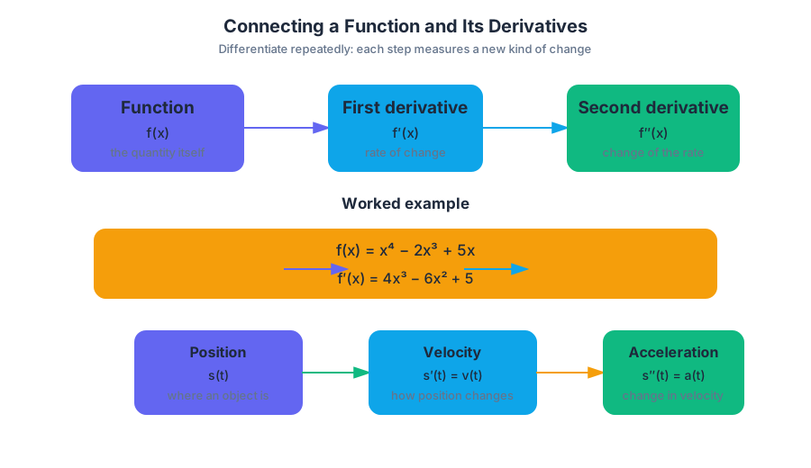
5.10 Introduction to Optimization Problems
Key concepts: Analytical applications of differentiation · Optimization problems · Absolute extrema · Local linearity in applied contexts · Interpreting functions in contextual situations
The common structure behind optimization problems: build an objective function, differentiate, analyze candidates on the feasible domain, and interpret the result in context.
5.10 Introduction to Optimization Problems
Many practical questions ask for a best value: the largest area, the lowest cost, the shortest time. The derivative tests from earlier in this unit already find the maximum or minimum of a given function. An optimization problem adds a step at each end: first build the function from a description, and afterwards interpret the answer in context.
Required Course Content: FUN-4 — “A function's derivative can be used to understand some behaviors of the function.”
Learning Objective FUN-4.B: “Calculate minimum and maximum values in applied contexts or analysis of functions.”
Suggested Skill 2.D: “Identify how mathematical characteristics or properties of functions are related in different representations.”
Suggested Skill 2.A: “Identify common underlying structures in problems involving different contextual situations.”
Optimization: the common structure behind different contexts
An optimization problem asks for the greatest or least value of a quantity: maximum area, minimum cost, greatest volume, shortest distance, or smallest error. Although the contexts look different, the mathematical structure is usually the same:
$$ \text{define an objective function} \longrightarrow \text{differentiate} \longrightarrow \text{analyze candidates} \longrightarrow \text{interpret the result}. $$
This shared structure is the focus of Suggested Skill 2.A: identify the underlying calculus pattern even when the story changes.
For a rectangle with perimeter $20$ units, let one side be $x$. The other side must be $10-x$, so the area is
$$ A(x)=x(10-x)=10x-x^2, \qquad 0\le x\le 10. $$
Differentiate:
$$ A'(x)=10-2x. $$
The critical value satisfies $A'(x)=0$, giving $x=5$. Since
$$ A''(x)=-2<0, $$
the area function is concave down, so the interior critical value produces a maximum. The dimensions are $5$ units by $5$ units, and the maximum area is
$$ A(5)=25\text{ square units}. $$
The derivative analysis supplies the mathematical conclusion; the context supplies its meaning. A complete solution must respect the feasible domain, identify what quantity is being optimized, and report the answer with appropriate units. That final interpretation develops Suggested Skill 3.F, explaining the meaning of mathematical solutions in context.
Retrieval check: If $g''(x)>0$ on an interval, what happens to the slopes of $g$, and what does that imply about the graph? If an optimization model has a critical value, why must its domain and endpoint behavior still be considered before declaring an absolute maximum?
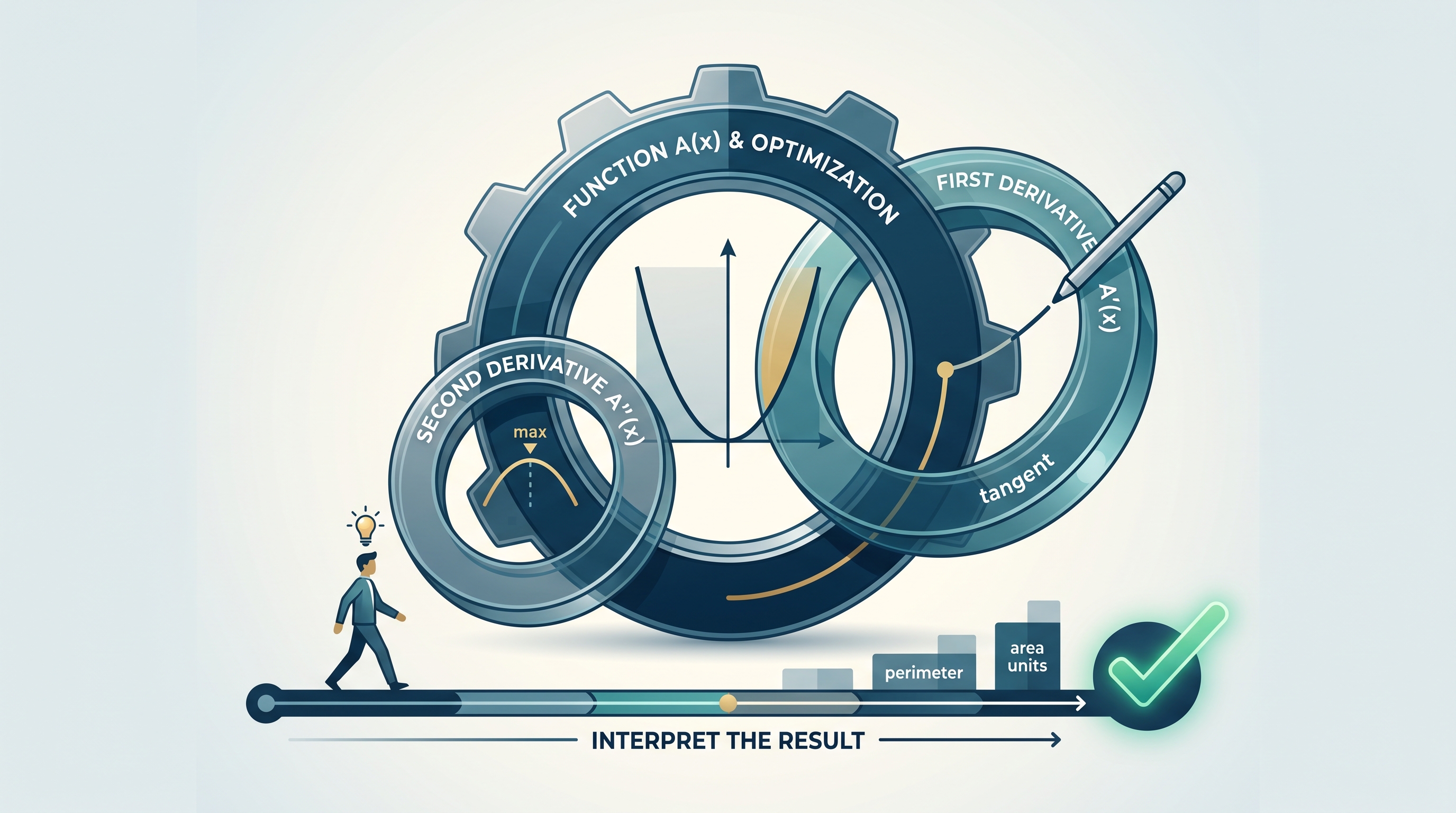
5.11 Solving Optimization Problems
Key concepts: Interpreting mathematical solutions in context · Solving optimization problems · Analytical applications of differentiation · Unit 5, Topic 5.11
A step-by-step method for solving optimization problems, from constraint and objective function to endpoint comparison and an answer interpreted in context with units.
5.11 Solving Optimization Problems
An optimization problem asks which allowable input makes a quantity as large or as small as possible, while an implicit relation describes how variables are linked even when one variable is not isolated as a function of the other. Both topics belong to Unit 5: Analytical Applications of Differentiation, where a derivative becomes a tool for proving and interpreting behavior.
5.11 Solving Optimization Problems
A mathematical answer is not complete until it is translated back into the situation. The value of a critical point may identify a dimension, time, or quantity, but the problem usually asks for something contextual: a maximum area, a minimum cost, or the dimensions that produce an optimum.
Interpret mathematical solutions in context: identify what the variable represents, check that the value is physically or logically allowed, evaluate the requested quantity, and state the conclusion with appropriate units.
Worked optimization: maximum area
A rectangle has perimeter $20$ centimeters. What dimensions produce the greatest possible area?
Let one side have length $x$ centimeters and the other have length $y$ centimeters. The perimeter condition gives
$$ 2x+2y=20, $$
so
$$ y=10-x. $$
Because side lengths cannot be negative, the meaningful domain is
$$ 0\le x\le 10. $$
The objective function—the quantity being optimized—is area:
$$ A(x)=xy=x(10-x)=10x-x^2. $$
Differentiate and locate the interior critical point:
$$ A'(x)=10-2x. $$
Set the derivative equal to zero:
$$ 10-2x=0 \quad\Longrightarrow\quad x=5. $$
The corresponding second side is
$$ y=10-5=5. $$
A global conclusion requires comparing the critical point with the endpoints of the closed interval:
$$ A(0)=0,\qquad A(5)=25,\qquad A(10)=0. $$
Therefore, the maximum area is
$$ \boxed{25\text{ cm}^2}, $$
and it occurs when the rectangle is a $5$-centimeter by $5$-centimeter square.
The number $5$ is a maximizing dimension; the number $25$ is the maximum area. Confusing these two answers is the wrong-output misconception: a correct derivative calculation can still lead to an incomplete contextual answer.
A reliable interpretation sequence
For an optimization problem, move through this chain:
- Define the variable and its units.
- Use the given constraint to write one variable in terms of the other.
- Build the objective function.
- Determine the feasible domain.
- Find critical values where the derivative is zero or undefined.
- Compare critical values and endpoints when the domain is closed.
- State the optimum in context, including units and the requested quantity.
This process develops 3.F Explain the meaning of mathematical solutions in context. It also uses 1.E Implementing Mathematical Processes, because the solver must select and execute appropriate differentiation and comparison procedures, and 3.E Justification, because the conclusion requires evidence rather than merely an answer.
Retrieval check
A rectangle has perimeter $20$ centimeters. Why must $A(5)$ be compared with $A(0)$ and $A(10)$? For the relation $x^2+y^2=25$, what geometric behavior occurs when $y=0$? A complete response should identify the endpoint comparison required for a global maximum and explain that $y=0$ produces vertical tangents.
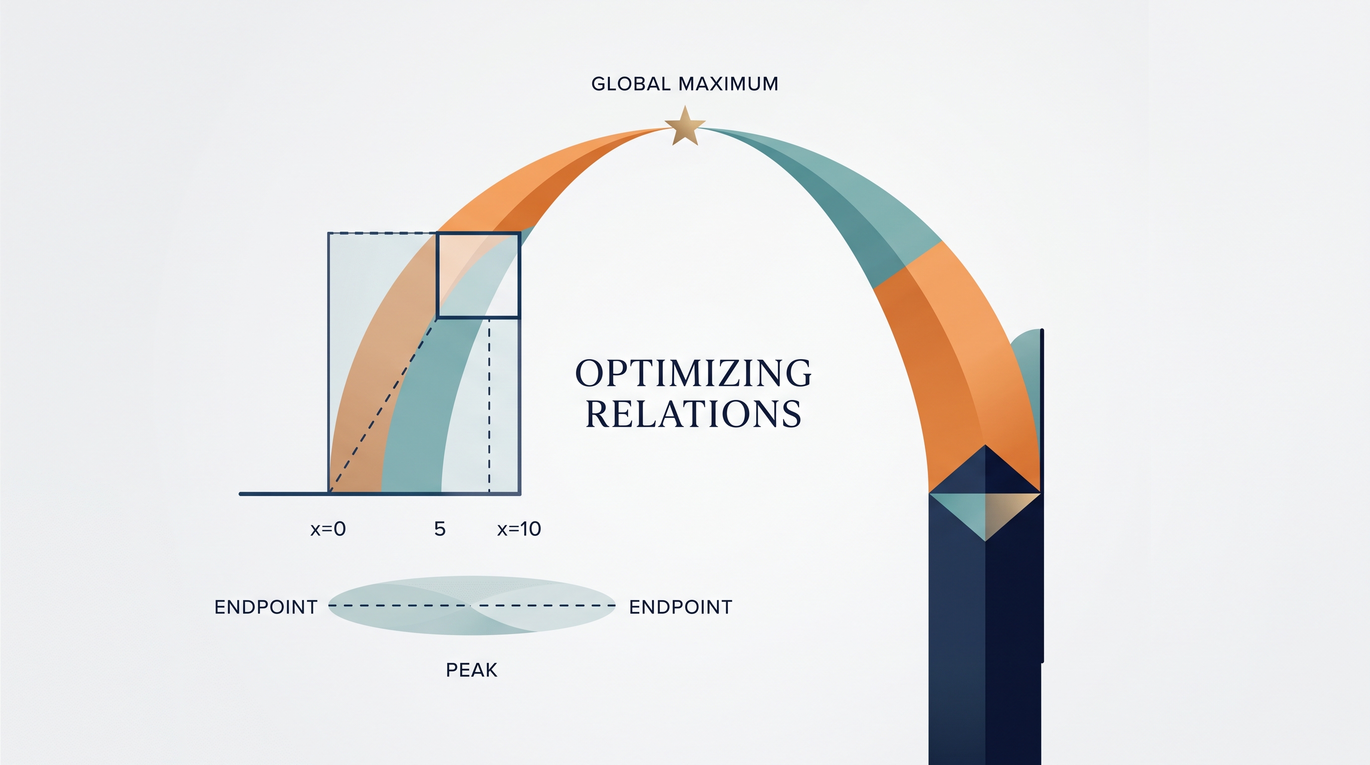
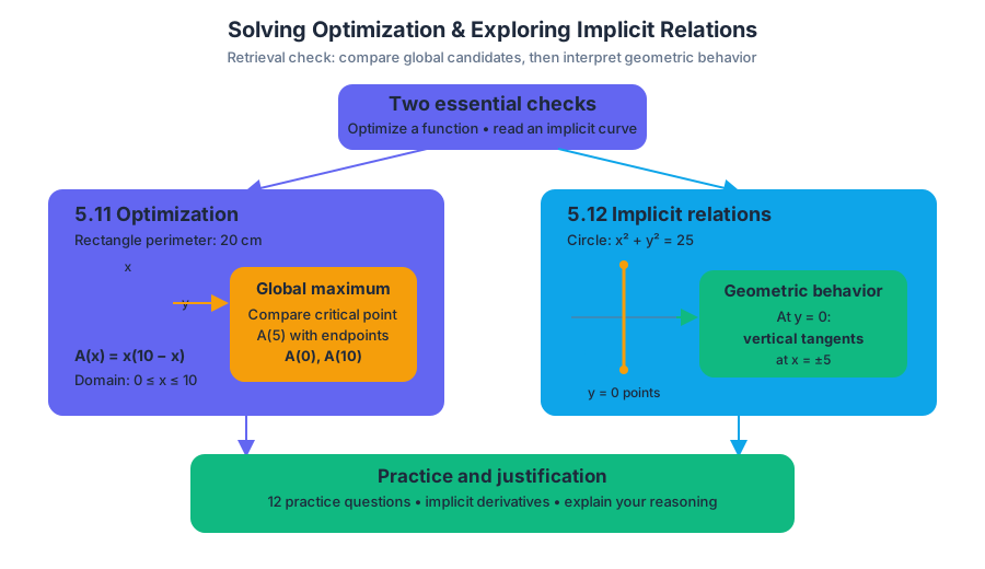
5.12 Exploring Behaviors of Implicit Relations
Key concepts: Exploring behaviors of implicit relations · Analytical applications of differentiation · Unit 5, Topic 5.12
How implicit differentiation reveals the behavior of an implicit relation, including local slopes and horizontal and vertical tangent lines.
5.12 Exploring Behaviors of Implicit Relations
Not every curve is the graph of a single function $y=f(x)$. A circle, for example, fails the vertical line test, yet it still has a tangent line at every point. This page shows how implicit differentiation lets you study the slopes and tangent behavior of such a relation without first solving for $y$.
5.12 Exploring Behaviors of Implicit Relations
An implicit relation connects $x$ and $y$ in an equation such as
$$ x^2+y^2=25, $$
without necessarily presenting $y$ explicitly as one formula in $x$. The relation is still analyzable: implicit differentiation reveals slopes, horizontal tangents, vertical tangents, and local behavior.
Differentiate both sides with respect to $x$. Since $y$ depends on $x$, differentiating $y^2$ requires the chain rule:
$$ 2x+2y\frac{dy}{dx}=0. $$
Solving for the slope gives
$$ \frac{dy}{dx}=-\frac{x}{y}. $$
At the point $(3,4)$, the tangent slope is
$$ \frac{dy}{dx}=-\frac{3}{4}. $$
Thus, near $(3,4)$, increasing $x$ corresponds locally to decreasing $y$.
The same derivative describes special tangent behavior. A horizontal tangent has slope $0$, so
$$ -\frac{x}{y}=0 $$
requires $x=0$ when $y\ne 0$. On the circle, this occurs at $(0,5)$ and $(0,-5)$. A vertical tangent occurs where the derivative expression is undefined because $y=0$; the corresponding points are $(5,0)$ and $(-5,0)$.
The division-by-$y$ misconception occurs when a student concludes that $\frac{dy}{dx}$ does not exist everywhere $y=0$, and therefore the curve has no tangent there. The formula $-\frac{x}{y}$ is undefined at those points, but the original differentiated equation,
$$ 2x+2y\frac{dy}{dx}=0, $$
shows that the tangent is vertical when $y=0$ and $x\ne 0$.
Exploring an implicit relation means connecting its equation, derivative, graph, and context. The derivative can identify where the curve rises or falls locally, where tangent lines are horizontal or vertical, and how the relation behaves without first solving explicitly for $y$.
The topic’s listed skills are 1.E Implementing Mathematical Processes—applying implicit-differentiation rules correctly—and 3.E Justification—using an equation, derivative, or geometric condition to support a conclusion. The governing enduring understanding is FUN-4: A function's derivative can be used to understand some behaviors of the function; implicit differentiation extends that behavioral analysis to relations that are not conveniently written as explicit functions.
Retrieval check
For the relation $x^2+y^2=25$, what is the slope of the tangent line at $(4,-3)$, and what geometric behavior occurs when $y=0$? A complete response should use $\dfrac{dy}{dx}=-\dfrac{x}{y}$ to find a slope of $\dfrac{4}{3}$ and explain that $y=0$ produces vertical tangents, even though the slope formula is undefined there.
Topic 5.12 also provides 12 practice questions for further work with implicit relations, especially derivative-based interpretation and justification.
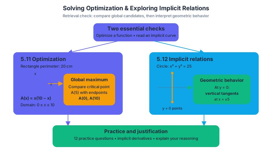
6.1 Exploring Accumulations of Change
Key concepts: Accumulation of change · Area under a curve as accumulation · Interpreting rates of change in context · Positive and negative rates and signed accumulation · Net change versus total change · Geometric area using straight-line graphs · Unit analysis for rates and accumulation · Velocity–time interpretation · Using tabulated data to approximate change
How a rate of change accumulates into a total change, read as signed area with units, and how net change differs from total change.
6.1 Exploring Accumulations of Change
A rate tells you how quickly a quantity changes; accumulating that rate over time tells you how much the quantity changes altogether. A faucet flowing at $4$ liters per second for $60$ seconds does not add “$4$ liters”—it adds approximately $4(60)=240$ liters.
From rate to accumulation
Accumulation is the total change produced by a rate over an interval. If $r(t)$ measures a rate of change and $t$ measures time, then the accumulated change is represented geometrically by the signed area between the graph of $r$ and the $t$-axis.
CHA-4.A: Interpret the meaning of an accumulation of change in a given context.
The sign matters. A rate above the axis is positive and produces positive accumulation; a rate below the axis is negative and produces negative accumulation.
For example, if $v(t)$ is velocity in meters per second and $t$ is measured in seconds, then the area under the velocity-versus-time graph has units
$$ \left(\frac{\text{meters}}{\text{second}}\right)(\text{seconds})=\text{meters}. $$
That area represents the particle’s change in position, or displacement. A positive area means the particle’s position increases; a negative area means its position decreases. The units are not an afterthought: multiplying the rate units by the independent-variable units is a powerful check on whether the interpretation is correct.
Net change versus total change
When a rate changes sign, two different quantities can be asked for:
- Net change combines positive and negative accumulation with their signs.
- Total change measures the entire amount transferred or traveled, so all pieces are counted positively.
Suppose a storage tank’s rate of change, $R(t)$, is measured in liters per second, with time in seconds. The following values describe a piecewise-constant approximation based on the rate at the left endpoint of each interval.
| Time interval (seconds) | Approximate rate (liters per second) | Signed accumulation (liters) |
|---|---|---|
| $0$ to $60$ | $4$ | $4(60)=240$ |
| $60$ to $90$ | $5$ | $5(30)=150$ |
| $90$ to $120$ | $3$ | $3(30)=90$ |
| $120$ to $135$ | $-1$ | $-1(15)=-15$ |
| $135$ to $150$ | $-2$ | $-2(15)=-30$ |
The net change is the signed sum:
$$ 240+150+90-15-30=435\text{ L}. $$
Thus, the tank gains approximately $435\text{ L}$ net over the $150$-second interval. The total amount transferred, however, counts both filling and draining:
$$ 240+150+90+15+30=525\text{ L}. $$
The tank does not gain $525\text{ L}$, because $45\text{ L}$ of that amount leaves the tank. The value $525\text{ L}$ describes total activity, while $435\text{ L}$ describes the final change in the tank’s contents.
Misconception check — “Area is always positive.”
Geometric area is often introduced as positive, but accumulation from a signed rate is not always positive. Regions below the axis contribute negative net change.
Skill focus and retrieval check
Topic 6.1 emphasizes Skill 4.B: Use appropriate units of measure. Topic 6.2 emphasizes Skill 1.F: Explain how an approximated value relates to the actual value. Together, these skills require more than a numerical calculation: identify what the area represents, attach correct units, preserve signs, and explain whether the approximation likely overestimates or underestimates the actual accumulation.
Retrieval check: A velocity graph has positive signed area $18\text{ m}$ from $t=0$ to $t=4$ and negative signed area $-7\text{ m}$ from $t=4$ to $t=6$. What are the particle’s net change in position and total distance traveled over the full interval?
Answer: The net change is
$$ 18-7=11\text{ m}, $$
while the total distance traveled is
$$ 18+7=25\text{ m}. $$
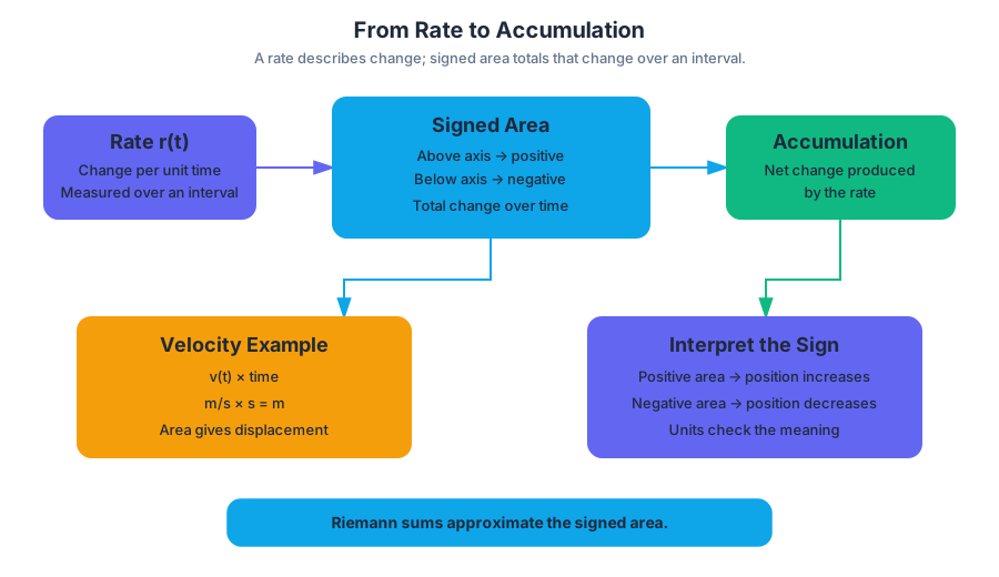
6.2 Approximating Areas with Riemann Sums
Key concepts: Approximating areas with Riemann sums · Area under a curve as accumulation · Using tabulated data to approximate change
How to approximate accumulated change with left and right Riemann sums, including unequal widths from a table, and how to tell over- from underestimates.
6.2 Approximating Areas with Riemann Sums
Topic 6.1 showed that accumulated change is the signed area under a rate graph. When the graph is curved, or the rate is known only at a few measured times, that area has no simple geometric formula. A Riemann sum approximates it with rectangles.
Suppose a storage tank’s rate of change, $R(t)$, is measured in liters per second, with time in seconds. The following values describe a piecewise-constant approximation based on the rate at the left endpoint of each interval.
| Time interval (seconds) | Approximate rate (liters per second) | Signed accumulation (liters) |
|---|---|---|
| $0$ to $60$ | $4$ | $4(60)=240$ |
| $60$ to $90$ | $5$ | $5(30)=150$ |
| $90$ to $120$ | $3$ | $3(30)=90$ |
| $120$ to $135$ | $-1$ | $-1(15)=-15$ |
| $135$ to $150$ | $-2$ | $-2(15)=-30$ |
Each row of the table is one rectangle: a rate held constant across an interval, times the width of that interval. Adding the signed column gives a net change of about $435$ L.
Approximating curved accumulation with rectangles
A rate graph is often curved rather than piecewise constant. To approximate its accumulation, divide the interval into subintervals, choose a representative rate on each subinterval, and form rectangles:
$$ \text{approximate accumulation} \approx (\text{rate})(\text{interval width}) + (\text{rate})(\text{interval width}) +\cdots $$
This procedure is a Riemann sum: a sum of rectangle areas used to approximate the area under a curve. Left-endpoint rectangles use the rate at the beginning of each subinterval; right-endpoint rectangles use the rate at the end. If the rate is increasing, left rectangles generally underestimate the positive accumulation, while right rectangles generally overestimate it.
The quality of an approximation depends on the rectangle widths and on how the function behaves. Narrower subintervals usually make the rectangles follow the curve more closely, but an approximation remains an approximation unless the exact accumulated value is determined by another method.
Applying the idea to data
For tabulated data at times $0$, $60$, $90$, $120$, $135$, and $150$ seconds, the interval widths are not all equal:
$$ 60,\quad 30,\quad 30,\quad 15,\quad 15. $$
Using one common width would misrepresent the accumulation. Each rate must be multiplied by the width of its own interval. In a real context, the result should be stated as a quantity and an interpretation—for example, “the tank gains approximately $435\text{ L}$ net,” rather than merely writing $435$.
Skill focus and retrieval check
Topic 6.2 emphasizes Skill 1.F: Explain how an approximated value relates to the actual value. Report the estimate with units, then say whether it is likely an overestimate or an underestimate, and why.
Retrieval check: A positive rate $r(t)$ is decreasing on $[0,6]$. With three equal subintervals, which is larger, the left or the right Riemann sum, and which one overestimates the accumulation? Answer: The left sum is larger and overestimates, because each left-endpoint height is the largest rate on its subinterval; the right sum underestimates.
6.3 Riemann Sums, Summation Notation, and Definite Integral Notation
Key concepts: Unit 6: Integration and Accumulation of Change · Definite integrals · Discrete models and limiting cases · Modeling real-world behavior through accumulation and change · AP Calculus AB and BC course expectations
How a Riemann sum in summation notation becomes the definite integral as a limit, and what each part of the integral notation means in context.
6.3 Riemann Sums, Summation Notation, and Definite Integral Notation
A finite sum can estimate accumulated change, but the definite integral gives the exact limiting accumulation when the partition becomes arbitrarily fine. The Fundamental Theorem of Calculus then reveals the remarkable fact that integration and differentiation undo one another.
From a finite sum to the definite integral
The approximation model established for Riemann sums can be compressed into summation notation. If a function $f$ is evaluated at sample points $x_i^*$ across subintervals of width $\Delta x$, then the accumulated approximation has the form
$$ \sum_{i=1}^{n} f(x_i^*)\Delta x. $$
As the number of subintervals increases and their widths approach zero, this sum approaches the exact accumulated value:
$$ \lim_{n\to\infty}\sum_{i=1}^{n} f(x_i^*)\Delta x
\int_a^b f(x),dx. $$
The symbol $\int_a^b f(x),dx$ is the definite integral of $f$ from $a$ to $b$. The lower bound $a$ and upper bound $b$ identify the interval, $f(x)$ is the rate or quantity being accumulated, and $dx$ indicates that the accumulation is taken with respect to $x$.
What the notation means in context
Suppose $r(t)$ is a rate measured in liters per minute. Then
$$ \int_0^5 r(t),dt $$
represents the total change in volume during the first $5$ minutes, measured in liters. If $r(t)$ is sometimes negative, the integral records net change: positive contributions add and negative contributions subtract.
Definite integral = accumulated signed change over an interval.
A discrete data set does not automatically justify a continuous integral. To replace observations at isolated times with $\int_a^b r(t),dt$, we assume that the rate varies continuously or that a reasonable continuous model, interpolation, or approximation represents the behavior between observations. The integral is therefore a limiting model of the underlying process, not merely a different notation for a table of measurements.
Misconception check
Misconception: “The integral always gives total amount.” A definite integral gives net accumulated change. If a rate becomes negative, its contribution reduces the result. Also, the bounds matter: $\int_a^b f(x),dx$ and $\int_b^a f(x),dx$ have opposite signs.
AP Calculus alignment and retrieval check
Topic 6.3 Riemann Sums, Summation Notation, and Definite Integral Notation chiefly develops Skill 2.C: Identify a re-expression of mathematical information presented in a given representation. The same accumulation can be written as a finite sum, as a limit of sums, or as a definite integral, and you should be able to move between those forms.
Retrieval check: Write $\lim_{n\to\infty}\sum_{i=1}^{n}\left(1+\frac{3i}{n}\right)^2\frac{3}{n}$ as a definite integral. The factor $\frac{3}{n}$ is $\Delta x$, so the interval has length $3$, and the sample points $x_i=1+\frac{3i}{n}$ are the right endpoints of the subintervals of $[1,4]$. The limit equals $\int_1^4 x^2,dx$.
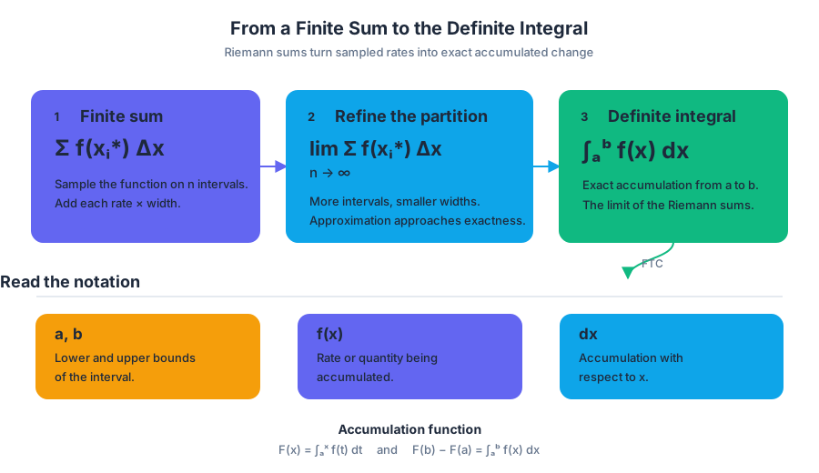
6.4 The Fundamental Theorem of Calculus and Accumulation Functions
Key concepts: Unit 6: Integration and Accumulation of Change · The relationship between integration and differentiation · The Fundamental Theorem of Calculus · Accumulation functions · Definite integrals · Modeling real-world behavior through accumulation and change · AP Calculus AB and BC course expectations
How accumulation functions are built from a moving upper limit, and how the Fundamental Theorem of Calculus ties their derivative back to the rate.
6.4 The Fundamental Theorem of Calculus and Accumulation Functions
A definite integral $\int_a^b f(x),dx$ gives one number: the net accumulation over a fixed interval. Let the upper endpoint move and the integral becomes a function. The Fundamental Theorem of Calculus says how fast that function changes, and in doing so it links integration to differentiation.
Accumulation functions
An accumulation function records how much change has built up from a fixed starting point. Given a rate function $f$, define
$$ A(x)=\int_a^x f(t),dt. $$
Here, $a$ is fixed while $x$ varies. The variable $t$ is a dummy variable: it identifies the input inside the integral, while $x$ identifies the current endpoint and therefore the input of the new function $A$.
For example, let $q(t)$ be the flow rate of water into a tank, in gallons per hour, and define
$$ V(t)=200+\int_0^t q(s),ds. $$
The tank begins with $200$ gallons. The integral gives the net volume added after $t$ hours, so $V(t)$ gives the tank’s total volume. Notice the structural relationship:
$$ V'(t)=q(t). $$
The derivative of the accumulated total is the current rate of accumulation.
The Fundamental Theorem of Calculus
The Fundamental Theorem of Calculus expresses the central relationship between integration and differentiation. In its accumulation-function form, if $f$ is continuous on an interval containing $a$, then
$$ A(x)=\int_a^x f(t),dt \quad\Longrightarrow\quad A'(x)=f(x). $$
This is the conceptual bridge between the two major operations of calculus:
$$ \text{rate of change} ;\xrightarrow{\text{integration}}; \text{accumulated change} $$
and
$$ \text{accumulated change} ;\xrightarrow{\text{differentiation}}; \text{rate of change}. $$
The second practical form evaluates a definite integral using an antiderivative. If $F'(x)=f(x)$, then
$$ \int_a^b f(x),dx=F(b)-F(a). $$
For the tank model, if $q(t)=3t^2+2$ gallons per hour, then an antiderivative is
$$ Q(t)=t^3+2t. $$
The amount of water added from $t=1$ to $t=4$ is
$$ \int_1^4(3t^2+2),dt
\left[t^3+2t\right]_1^4
(64+8)-(1+2)
$$
Thus, $69$ gallons enter the tank during that interval.
The first FTC application differentiates an accumulation function; the second evaluates an accumulated quantity using an antiderivative.
Misconception check
Misconception: “The integral always gives total amount.” A definite integral gives net accumulated change. If a rate becomes negative, its contribution reduces the result. Also, the bounds matter: $\int_a^b f(x),dx$ and $\int_b^a f(x),dx$ have opposite signs.
A second common error is writing an accumulation function as $\int_a^x f(x),dx$. The same symbol cannot clearly serve as both the moving endpoint and the integration variable. Write $\int_a^x f(t),dt$ instead.
AP Calculus alignment and retrieval check
Topics 6.3 Riemann Sums, Summation Notation, and Definite Integral Notation and 6.4 The Fundamental Theorem of Calculus and Accumulation Functions are core AP Calculus AB and BC expectations within Unit 6: Integration and Accumulation of Change, weighted approximately 17–20% of either exam. They chiefly develop Skill 2.C: Identify a re-expression of mathematical information presented in a given representation and Skill 1.D: Identify an appropriate mathematical rule or procedure based on the relationship between concepts. They also require Mathematical Practice 1—Implementing Mathematical Processes, Mathematical Practice 2—Connecting Representations, Mathematical Practice 3—Justification, and Mathematical Practice 4—Communication and Notation.
Retrieval check: If $B(x)=\int_2^x (u^3-1),du$, identify $B'(x)$ and explain what $\int_2^5(u^3-1),du$ represents. The answers are
$$ B'(x)=x^3-1 $$
and the net accumulation of the rate $u^3-1$ from $u=2$ to $u=5$.
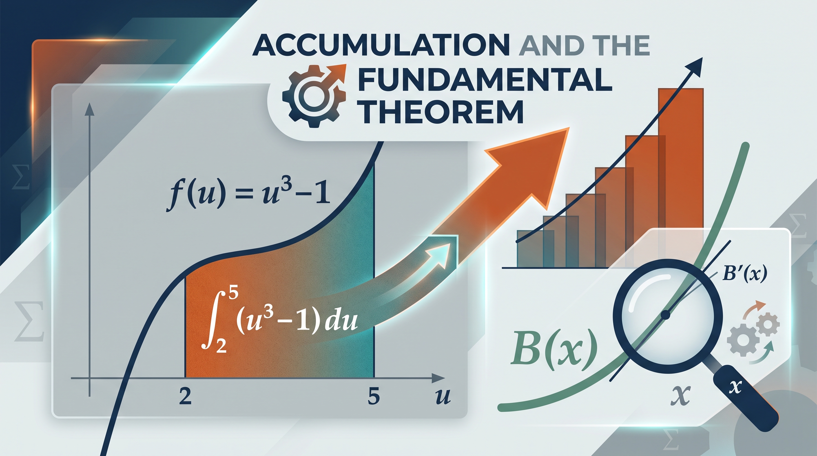
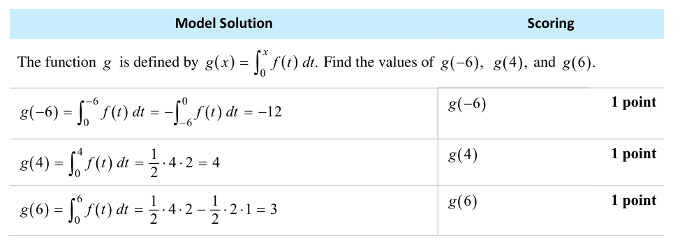
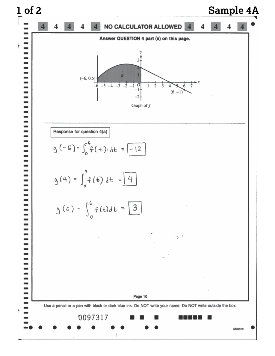
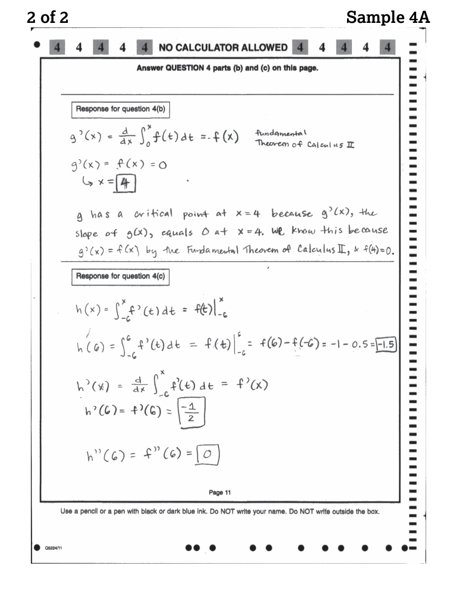
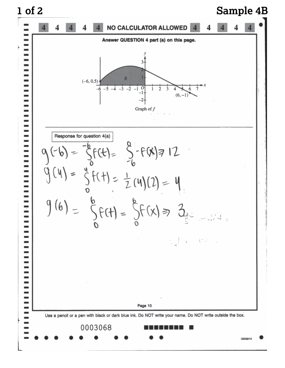
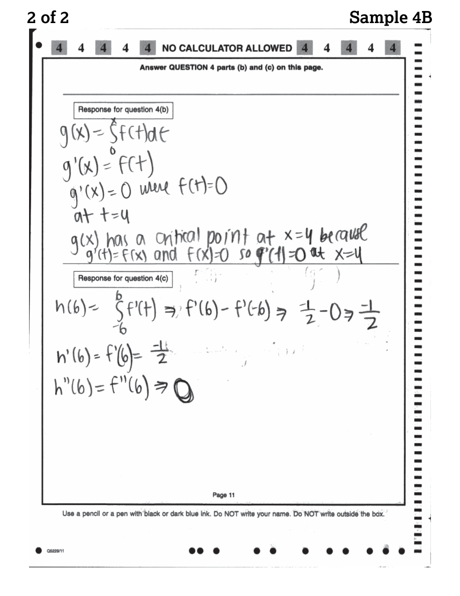
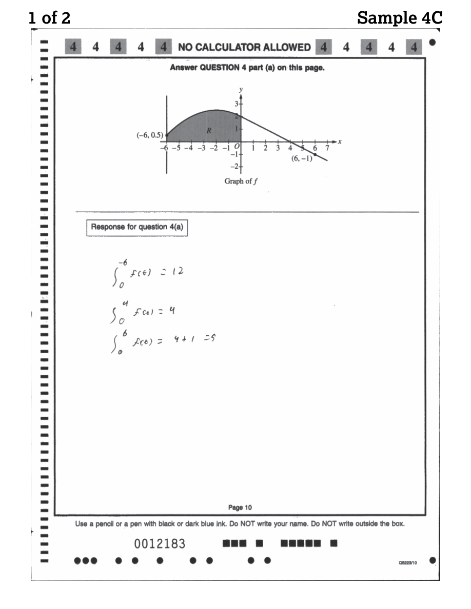
6.5 Interpreting the Behavior of Accumulation Functions Involving Area
Key concepts: Accumulation functions defined by definite integrals · Interpreting accumulation functions involving area · Accumulation of change · Using definite integrals to define new functions · Differentiating accumulation functions · Relating mathematical characteristics across representations
How to read where an accumulation function rises, falls, bends and has extrema from the graph of its rate, using signed area for its values.
6.5 Interpreting the Behavior of Accumulation Functions Involving Area
An accumulation graph can stay high even while its associated rate is negative: it is falling, but from the larger value that earlier positive accumulation built up. The key question is not merely “How much area is present?” but which signed areas are being added, and how do they change the function’s behavior?
Reading an accumulation function through its rate
Suppose $G(x)$ records the net amount accumulated from a starting location to $x$, while $f(x)$ is the rate being accumulated. The load-bearing relationship from the preceding topic is
$$G'(x)=f(x).$$
This single connection lets us translate between representations:
| Information about $f$ | Consequence for $G$ |
|---|---|
| $f(x)>0$ | $G$ is increasing |
| $f(x)<0$ | $G$ is decreasing |
| $f(x)=0$ | $G$ has a horizontal tangent, possibly a local extremum |
| $f$ is increasing | $G$ is concave up |
| $f$ is decreasing | $G$ is concave down |
The word net matters. Area above the $x$-axis contributes positively, while area below the $x$-axis contributes negatively. Thus, a definite integral can represent both accumulated change and signed area—not always ordinary geometric area.
Worked interpretation: area controls the graph
Let
$$G(x)=\int_0^x f(t),dt,$$
where the graph of $f$ is below the $x$-axis on $0<x<3$, crosses the axis at $x=3$, and is above the axis on $3<x<6$. Without calculating an antiderivative, interpret $G$.
Because $f(x)<0$ on $(0,3)$, $G$ decreases there. At $x=3$, the accumulation graph has a horizontal tangent because $f(3)=0$. Since $f(x)>0$ on $(3,6)$, $G$ increases there. Therefore, $G$ has a local minimum at $x=3$, provided the sign changes from negative to positive.
If the region below the axis from $0$ to $3$ has area $8$ and the region above the axis from $3$ to $5$ has area $11$, then
$$G(3)=-8$$
and
$$G(5)=-8+11=3.$$
The function does not “forget” the first region: the later positive area first cancels the earlier deficit and then creates a positive net accumulation.
When the upper limit is a function of $x$
When an accumulation expression contains a variable limit, differentiate it to reveal the matching rate. For example, if
$$H(x)=\int_2^{x^3}\sqrt{1+t^2},dt,$$
then the variable endpoint contributes a chain-rule factor:
$$H'(x)=\sqrt{1+(x^3)^2}\cdot 3x^2 =3x^2\sqrt{1+x^6}.$$
The common error is to write only $\sqrt{1+x^6}$ and forget that the upper limit is $x^3$, not $x$. This is the missing chain-factor misconception: a variable boundary changes at its own rate.
Skill focus and retrieval check
These tasks explicitly develop 2.D Identify how mathematical characteristics or properties of functions are related in different representations, especially when a graph of $f$, an accumulation graph $G$, and an integral communicate the same behavior. They also develop 3.D Apply an appropriate mathematical definition, theorem, or test when using signed area, integral properties, and derivative-based behavior.
Retrieval check: If $f$ is negative and decreasing on an interval, what must be true about $G$ there, where $G'(x)=f(x)$? Answer: $G$ is decreasing and concave down. If $\int_0^4 f(x),dx=6$ and $\int_4^7 f(x),dx=-9$, then $\int_7^0 f(x),dx=3$.
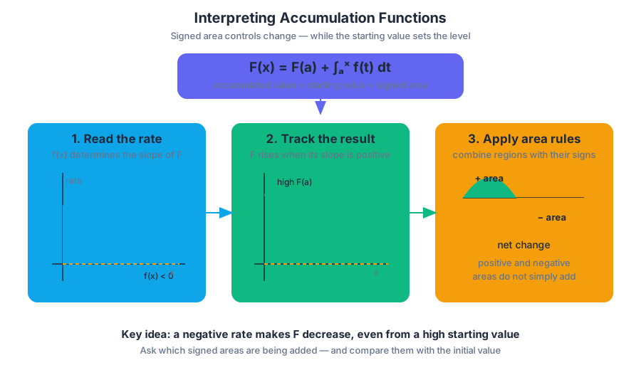
6.6 Applying Properties of Definite Integrals
Key concepts: Applying properties of definite integrals · Calculating definite integrals · Connecting definite integrals with Riemann sums · Breaking complex expressions into familiar components
The algebraic properties of definite integrals: linearity, reversing bounds and adding adjacent intervals, used to get new values from known ones.
6.6 Applying Properties of Definite Integrals
An accumulation function is built from a definite integral, so anything that simplifies definite integrals also simplifies the work of Topic 6.5. This page collects the algebraic properties that let you scale, split, combine and reverse integrals whose values you already know, often without ever finding a formula for $f$.
Properties of definite integrals: simplify before calculating
Definite integrals obey algebraic properties that allow a complicated expression to be separated into familiar components:
$$\int_a^b \left[c f(x)+d g(x)\right],dx
c\int_a^b f(x),dx+d\int_a^b g(x),dx.$$
Reversing the bounds changes the sign,
$$\int_b^a f(x),dx=-\int_a^b f(x),dx,$$
and adjacent intervals can be combined:
$$\int_a^c f(x),dx+\int_c^b f(x),dx
\int_a^b f(x),dx.$$
For example, if
$$\int_1^4 f(x),dx=7 \qquad\text{and}\qquad \int_4^6 f(x),dx=-2,$$
then
$$\int_6^1 f(x),dx
-\int_1^6 f(x),dx
-\left(7+(-2)\right) =-5.$$
This is often faster and safer than attempting to find a formula for $f$. Break complex expressions into known pieces, preserve coefficients, and check the direction of every interval.
Two more facts round out the list. An integral over an interval of zero width is zero: $\int_a^a f(x),dx=0$. And linearity combines known values: if $\int_1^4 f(x),dx=7$ and $\int_1^4 g(x),dx=3$, then $\int_1^4\left[2f(x)-5g(x)\right]dx=2(7)-5(3)=-1$.
Connecting a definite integral with a formula
Sometimes a limit of a Riemann sum or a definite integral is disguised inside a complicated expression. The strategic move is to identify the integrand and its interval. For instance,
$$\lim_{n\to\infty}\sum_{i=1}^{n} \left(3+\frac{2i}{n}\right)^2\frac{1}{n} $$
matches
$$\int_0^1 (3+2x)^2,dx.$$
The factor $\frac{1}{n}$ supplies the subinterval width, and $3+\frac{2i}{n}$ supplies sample inputs in the interval $[0,1]$. Conversely, an integral can be recognized as accumulated change whenever its integrand has rate units and its differential supplies the input interval.
Skill focus and retrieval check
These tasks explicitly develop 2.D Identify how mathematical characteristics or properties of functions are related in different representations, especially when a graph of $f$, an accumulation graph $G$, and an integral communicate the same behavior. They also develop 3.D Apply an appropriate mathematical definition, theorem, or test when using signed area, integral properties, and derivative-based behavior.
Retrieval check: If $f$ is negative and decreasing on an interval, what must be true about $G$ there, where $G'(x)=f(x)$? Answer: $G$ is decreasing and concave down. If $\int_0^4 f(x),dx=6$ and $\int_4^7 f(x),dx=-9$, then $\int_7^0 f(x),dx=3$.
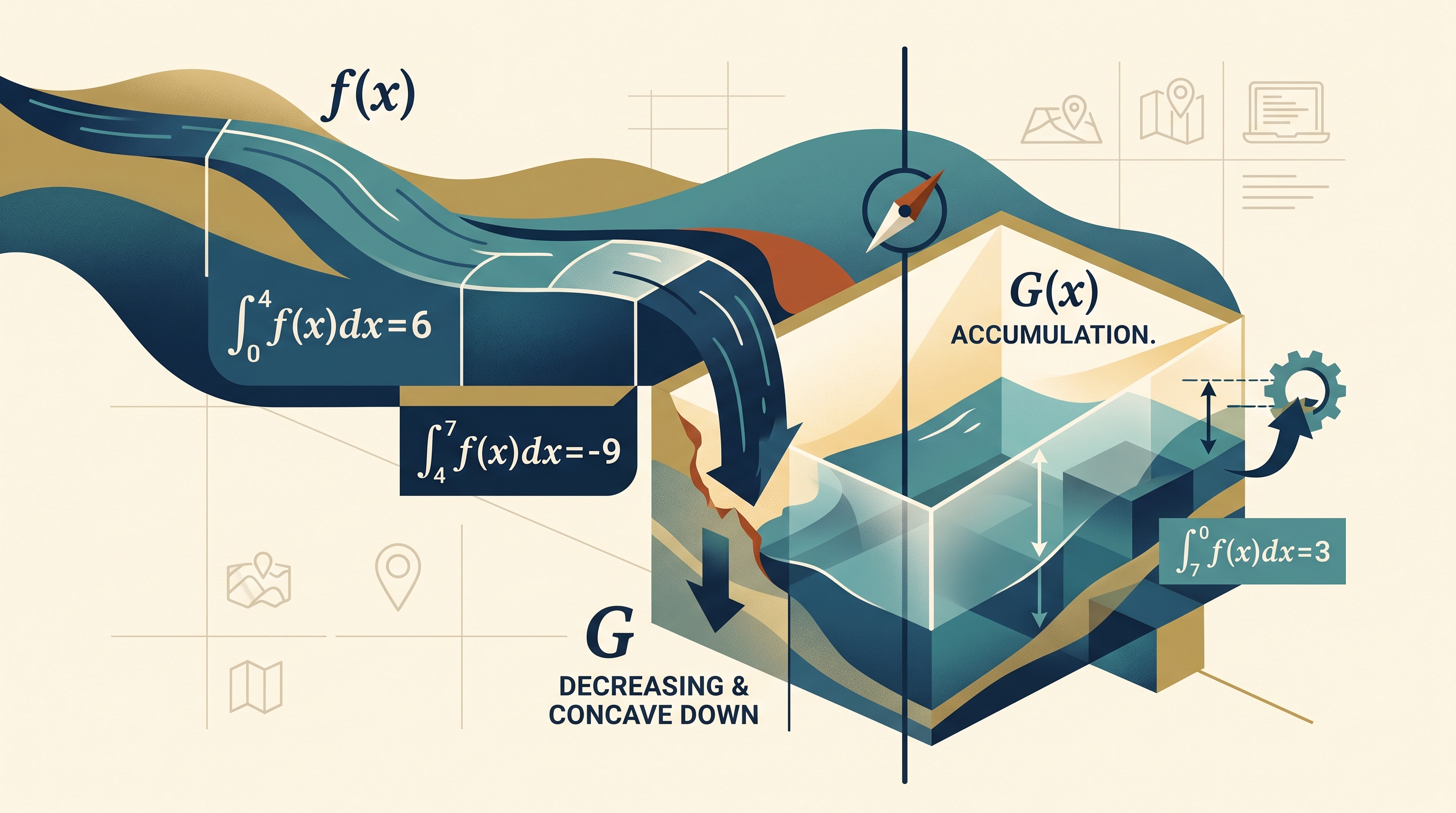
6.7 The Fundamental Theorem of Calculus and Definite Integrals
Key concepts: Definition of an antiderivative: a function whose derivative is the given function · The Fundamental Theorem of Calculus connecting derivatives and definite integrals · Evaluating a definite integral using an antiderivative · Definite integrals and accumulation of change
How the Fundamental Theorem of Calculus evaluates a definite integral as the endpoint difference $F(b)-F(a)$ of an antiderivative.
6.7 The Fundamental Theorem of Calculus and Definite Integrals
A definite integral measures accumulated change, while an antiderivative reverses differentiation. The Fundamental Theorem of Calculus connects these two ideas: instead of adding infinitely many tiny contributions directly, we can find a function whose derivative is the integrand and evaluate that function at the endpoints.
If $F'(x)=f(x)$, then $F$ is an antiderivative of $f$.
Finding antiderivatives is the work of Topic 6.8; this page is about what to do once you have one. For a polynomial, reverse the power rule term by term: an antiderivative of $4x^3-6x+5$ is $x^4-3x^2+5x$, which you can confirm by differentiating.
The Fundamental Theorem evaluates definite integrals
If $f$ is continuous on $[a,b]$ and $F$ is an antiderivative of $f$, then the evaluation part of the Fundamental Theorem of Calculus states $$ \int_a^b f(x),dx=F(b)-F(a). $$ The definite integral is therefore an endpoint difference, not an indefinite family.
Worked example. Evaluate $$ \int_1^3 \left(4x^3-6x+5\right),dx. $$ An antiderivative is $$ F(x)=x^4-3x^2+5x. $$ Apply the endpoint rule: $$ \int_1^3 \left(4x^3-6x+5\right),dx =F(3)-F(1). $$ Compute: $$ F(3)=81-27+15=69, $$ $$ F(1)=1-3+5=3. $$ Therefore, $$ \boxed{\int_1^3 \left(4x^3-6x+5\right),dx=69-3=66}. $$
Although the antiderivative may be written as $F(x)+C$, the constant disappears in the endpoint difference: $$ [F(b)+C]-[F(a)+C]=F(b)-F(a). $$ That is why $+C$ is required for an indefinite integral but is not written in the final evaluation of a definite integral.
Accumulation and the first part of the Fundamental Theorem
If $f$ is continuous on an interval containing $a$, define an accumulation function by $$ F(x)=\int_a^x f(t),dt. $$ The Fundamental Theorem states $$ \frac{d}{dx}\left(\int_a^x f(t),dt\right)=f(x). $$ The variable $t$ is a temporary integration variable; the variable $x$ determines the moving endpoint. This result proves that the accumulation function itself is an antiderivative of $f$, matching FUN-6.B.2.
AP alignment and retrieval check
This topic develops FUN-6: Recognizing opportunities to apply knowledge of geometry and mathematical rules can simplify integration, FUN-6.B: Evaluate definite integrals analytically using the Fundamental Theorem of Calculus, and FUN-6.B.1, FUN-6.B.2, FUN-6.B.3. It also develops FUN-6.C: Determine antiderivatives of functions and indefinite integrals, using knowledge of derivatives, including FUN-6.C.1 and FUN-6.C.2. The relevant AP skill is 3.D: Apply an appropriate mathematical definition, theorem, or test—here, selecting and applying the Fundamental Theorem with correct notation and endpoint evaluation.
Retrieval check: If a proposed antiderivative of $f(x)$ is $G(x)$, differentiate $G(x)$ and compare the result with $f(x)$. If they match, $G(x)+C$ describes the full indefinite-integral family. For a definite integral, use $G(b)-G(a)$; the two constants cancel.
6.8 Finding Antiderivatives and Indefinite Integrals: Basic Rules and Notation
Key concepts: Antiderivatives as the inverse process of differentiation · Definition of an antiderivative: a function whose derivative is the given function · Indefinite integral notation and the constant of integration · The family of antiderivatives differs by an arbitrary constant C · Finding antiderivatives using basic integration rules · Verifying antiderivatives by differentiating them
What antiderivatives and indefinite integrals are, why they carry a constant of integration, and the basic rules for finding them by reversing derivative rules.
6.8 Finding Antiderivatives and Indefinite Integrals: Basic Rules and Notation
Differentiation starts with a function and produces its rate of change. This topic runs that process backwards: given a rate, find a function it could have come from. That function is an antiderivative, and its notation and basic rules are the working tools for every integral in the rest of the unit.
If $F'(x)=f(x)$, then $F$ is an antiderivative of $f$.
Differentiation and antidifferentiation as inverse processes
Differentiation takes a function and produces its rate of change. Antidifferentiation asks the reverse question: “Which function has this derivative?” For example, because $$ \frac{d}{dx}\left(x^3\right)=3x^2, $$ the function $x^3$ is an antiderivative of $3x^2$.
The reverse process is not unique. Every function of the form $x^3+C$ has derivative $3x^2$, because the derivative of any constant is zero: $$ \frac{d}{dx}\left(x^3+C\right)=3x^2. $$ Thus, antiderivatives come as a family of functions separated vertically by constant amounts.
Indefinite integrals and the constant of integration
The notation $$ \int f(x),dx $$ is an indefinite integral. It represents the entire family of antiderivatives of $f$, not one particular function. Formally, if $F'(x)=f(x)$, then $$ \int f(x),dx=F(x)+C, $$ where $C$ represents any constant of integration.
For instance, $$ \int 6x^2,dx=2x^3+C, $$ because $$ \frac{d}{dx}\left(2x^3+C\right)=6x^2. $$ The symbol $dx$ identifies the variable of integration. It also reminds us that the operation is connected to reversing differentiation with respect to $x$.
A common misconception is “the constant does not matter, so it can be omitted.” The constant does not affect the derivative, but omitting $+C$ incorrectly turns a family of answers into a single answer. An initial condition, such as $F(2)=5$, can later determine one specific value of $C$.
Basic rules for finding antiderivatives
Differentiation rules provide the foundation for finding antiderivatives. Reverse the power rule: $$ \int x^n,dx=\frac{x^{n+1}}{n+1}+C,\qquad n\ne -1. $$ Use linearity to integrate sums, differences, and constant multiples term by term: $$ \int \left[af(x)+bg(x)\right],dx =a\int f(x),dx+b\int g(x),dx. $$
The basic antiderivatives associated with familiar derivative rules include $$ \int \cos x,dx=\sin x+C, $$ $$ \int \sin x,dx=-\cos x+C, $$ $$ \int e^x,dx=e^x+C, $$ and $$ \int \frac{1}{x},dx=\ln|x|+C. $$
Worked example. Find an indefinite integral: $$ \int \left(4x^3-6x+5\right),dx. $$ Integrate each term: $$ \int 4x^3,dx-\int 6x,dx+\int 5,dx =x^4-3x^2+5x+C. $$ Verification gives $$ \frac{d}{dx}\left(x^4-3x^2+5x+C\right)=4x^3-6x+5, $$ the original integrand, because the constant $C$ has derivative $0$. Therefore, $$ \boxed{\int \left(4x^3-6x+5\right),dx=x^4-3x^2+5x+C}. $$
AP alignment and retrieval check
This topic develops FUN-6.C: Determine antiderivatives of functions and indefinite integrals, using knowledge of derivatives, including FUN-6.C.1 and FUN-6.C.2. The suggested AP skill is 4.C: Use appropriate mathematical symbols and notation. Every basic rule here is a derivative rule read in reverse, and the notation carries meaning: write $dx$, and keep $+C$ on every indefinite integral.
Retrieval check: If a proposed antiderivative of $f(x)$ is $G(x)$, differentiate $G(x)$ and compare the result with $f(x)$. If they match, $G(x)+C$ describes the full indefinite-integral family. For a definite integral, use $G(b)-G(a)$; the two constants cancel.
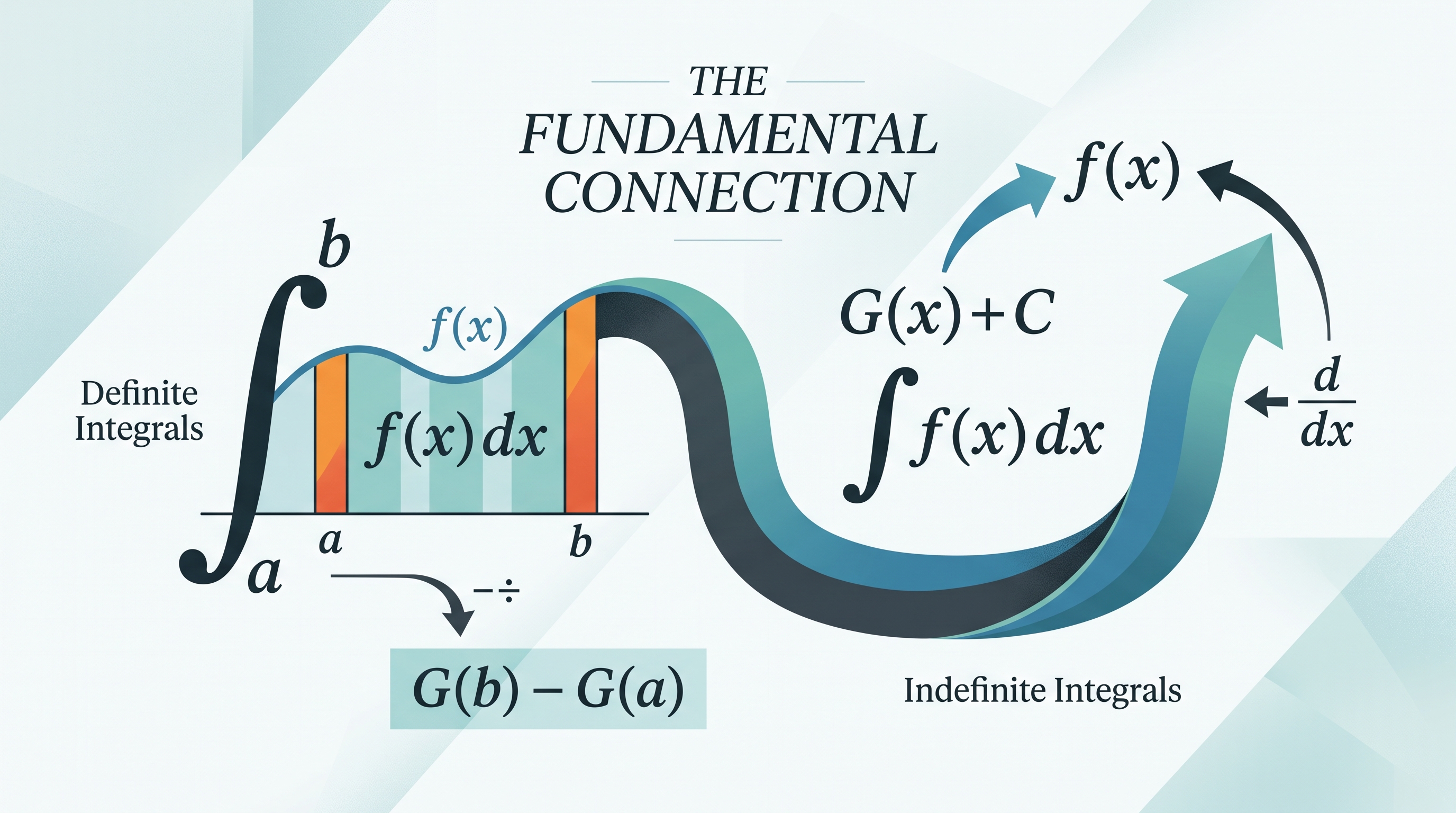
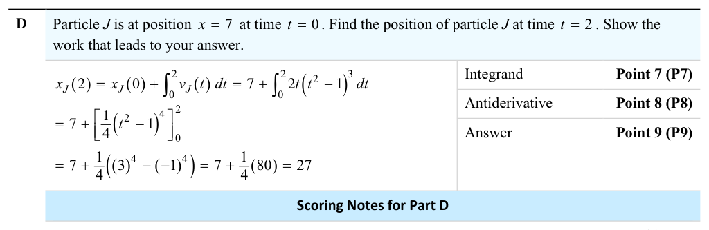
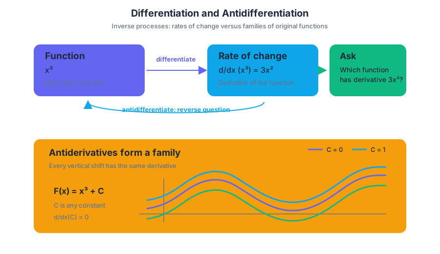
6.9 Integrating Using Substitution
Key concepts: Integration by substitution (u-substitution) · Recognizing integrands that involve the chain rule · Finding indefinite integrals · Evaluating definite integrals · Interpreting constants correctly when evaluating definite integrals · Using a structured multistep process for substitution · Applying mathematical rules and procedures with or without technology
How to integrate by $u$-substitution, including changing the bounds of a definite integral and handling constants written outside the integral.
6.9 Integrating Using Substitution
The integral $\int 2t(t^2-1)^3,dt$ looks complicated only until you notice that $2t$ is the derivative of $t^2-1$. Integration by substitution reverses the chain rule by replacing a repeated inner expression with one simpler variable.
The central pattern: recognize a reversed chain rule
If an integrand contains a function and its derivative, substitution is often the cleanest procedure. Let $$ u=t^2-1. $$ Then $$ du=2t,dt. $$ The integral becomes $$ \int 2t(t^2-1)^3,dt =\int u^3,du =\frac14u^4+C =\frac14(t^2-1)^4+C. $$
The substitution works because it compresses the complicated expression $t^2-1$ into the single variable $u$. After integrating in $u$, substitute back so that the antiderivative is expressed in the original variable.
A reliable substitution pipeline
Use the following visual decision path whenever an integrand appears to contain a composite function:
- Identify the repeated inner expression, such as $t^2-1$.
- Set that expression equal to $u$.
- Compute $du$, including its differential factor.
- Rewrite every relevant part of the integral using $u$ and $du$.
- Integrate with respect to $u$.
- Substitute the original expression back.
- Differentiate the result mentally or algebraically to check it.
For example, $$ \int 6x(x^2+4)^2,dx $$ suggests $u=x^2+4$, so $du=2x,dx$ and $6x,dx=3,du$. Therefore, $$ \int 6x(x^2+4)^2,dx =3\int u^2,du =u^3+C =(x^2+4)^3+C. $$
Key insight: A substitution is not a symbol-swapping trick. It is a deliberate attempt to match the structure of the chain rule in reverse.
Definite integrals and the bounds
For a definite integral, substitution can be completed in either of two consistent ways: substitute back into the original variable and use the original bounds, or change the bounds into $u$-values and remain in $u$ throughout.
Evaluate $$ \int_0^2 2t(t^2-1)^3,dt. $$ With $u=t^2-1$ and $du=2t,dt$, the bounds become $$ t=0\Rightarrow u=-1, \qquad t=2\Rightarrow u=3. $$ Thus, $$ \int_0^2 2t(t^2-1)^3,dt =\int_{-1}^{3}u^3,du =\left[\frac14u^4\right]_{-1}^{3} =\frac14(3^4)-\frac14((-1)^4) =20. $$
Alternatively, the antiderivative in terms of $t$ is $$ \frac14(t^2-1)^4, $$ so $$ \left[\frac14(t^2-1)^4\right]_0^2=20. $$ Both methods agree because they describe the same accumulation.
Constants outside versus inside an integral
Parentheses and placement matter. A number written after the definite-integral expression is outside the integral; a number inside the integrand is accumulated over the interval.
Using $v_J(t)=2t(t^2-1)^3$, interpret $$ \int_0^2 v_J(t),dt+7. $$ The $+7$ is outside the integral, so $$ \int_0^2 v_J(t),dt+7
\left[\frac14(t^2-1)^4\right]_0^2+7. $$ It is not $$ \left[\frac14(t^2-1)^4+7t\right]_0^2, $$ because that expression treats $7$ as part of the integrand, effectively integrating $v_J(t)+7$.
Misconception check — “Every term near the integral sign is integrated.”
False. In $\int_a^b f(t),dt+7$, only $f(t)$ is integrated. In $\int_a^b\bigl(f(t)+7\bigr),dt$, both terms are integrated.
AP skill and retrieval check
This topic develops Mathematical Practice 1, Skill 1.E: “Apply appropriate mathematical rules or procedures, with and without technology.” The procedure is not merely calculating: the important decision is selecting substitution, long division, completing the square, or an equivalent algebraic form.
Retrieval check: Evaluate $$ \int_1^3 6x(x^2+4)^2,dx+5. $$ The correct antiderivative is $$ (x^2+4)^3, $$ so, because $+5$ is outside the integral, the result is $$ \left[(x^2+4)^3\right]_1^3+5 =(13^3-5^3)+5 =2187+5 =2192. $$ Writing $\left[(x^2+4)^3+5x\right]_1^3$ would incorrectly place the constant inside the integrand.
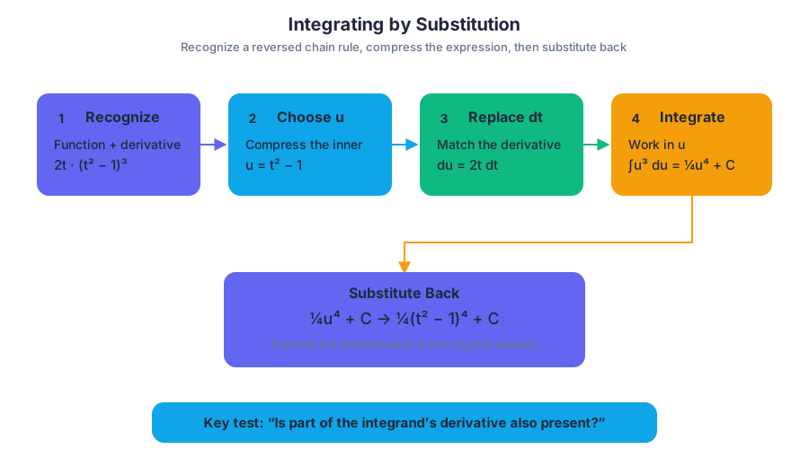
6.10 Integrating Functions Using Long Division and Completing the Square
Key concepts: Using equivalent algebraic rearrangements to simplify integration · Finding indefinite integrals · Evaluating definite integrals · Integrating functions using polynomial long division · Completing the square before integrating · Applying mathematical rules and procedures with or without technology
How polynomial long division and completing the square rewrite a rational integrand into forms whose antiderivatives are already known.
6.10 Integrating Functions Using Long Division and Completing the Square
Substitution handles integrands that contain an inner expression together with its derivative. Many rational integrands have no such pair, yet they become routine once the algebra is rewritten. Two rearrangements matter most here: polynomial long division and completing the square.
When algebra must come before integration
Some integrands do not immediately match a basic antiderivative rule. The enduring understanding FUN-6 is that recognizing opportunities to apply mathematical rules can simplify integration. The learning objective FUN-6.D requires determining indefinite integrals and evaluating definite integrals for integrands requiring substitution or rearrangement into equivalent forms. Essential knowledge FUN-6.D.3 specifically includes rearrangements such as polynomial long division and completing the square.
Polynomial long division
When the numerator has degree at least as large as the denominator, divide first. For $$ \int \frac{x^2+3x+2}{x+1},dx, $$ polynomial division gives $$ \frac{x^2+3x+2}{x+1}=x+2. $$ Therefore, $$ \int \frac{x^2+3x+2}{x+1},dx =\int(x+2),dx =\frac12x^2+2x+C. $$ The division exposes an integrand whose terms have familiar antiderivatives.
Division usually leaves a remainder, and a constant remainder over a linear divisor integrates to a logarithm. For example, $\frac{x^2+1}{x+1}=x-1+\frac{2}{x+1}$, so $\int\frac{x^2+1}{x+1},dx=\frac12x^2-x+2\ln|x+1|+C$.
Completing the square
A quadratic can often be rewritten into a form that makes substitution or a standard inverse-tangent pattern visible: $$ x^2+6x+13=(x+3)^2+4. $$ Thus, $$ \int\frac{dx}{x^2+6x+13}
\int\frac{dx}{(x+3)^2+2^2}
\frac12\arctan\left(\frac{x+3}{2}\right)+C. $$ The algebraic rearrangement does not change the function; it changes the function’s appearance so an integration rule can be applied.
AP skill and retrieval check
This topic develops Mathematical Practice 1, Skill 1.E: “Apply appropriate mathematical rules or procedures, with and without technology.” The procedure is not merely calculating: the important decision is selecting substitution, long division, completing the square, or an equivalent algebraic form.
Retrieval check: Which rearrangement comes first for $\int\frac{x^3}{x-1},dx$, and which for $\int\frac{dx}{x^2-4x+8}$? In the first, the numerator's degree exceeds the denominator's, so divide: $\frac{x^3}{x-1}=x^2+x+1+\frac{1}{x-1}$. In the second, complete the square: $x^2-4x+8=(x-2)^2+4$, which gives $\frac12\arctan\left(\frac{x-2}{2}\right)+C$.
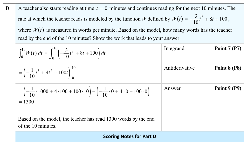
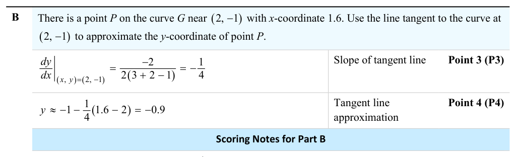
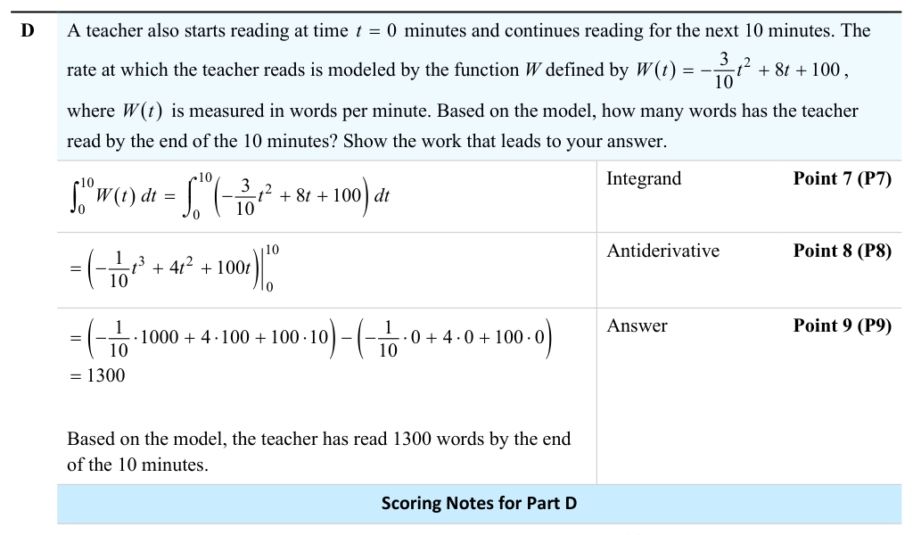
6.11 Integrating Using Integration by Parts (BC only)
Key concepts: Integration by parts (BC only) · Recognizing when an integrand benefits from integration by parts · Using the product rule in reverse to derive integration by parts
How integration by parts reverses the product rule, how to choose $u$ and $dv$, and a worked evaluation of $\int xe^x\,dx$.
6.11 Integrating Using Integration by Parts (BC only)
Some integrals become easy only after you reverse a familiar differentiation pattern: the product rule leads to integration by parts, while a complicated rational expression can be split into simpler fractions through linear partial fractions. Both techniques are designated BC only.
Integration by parts: reversing the product rule
The product rule says
$$ \frac{d}{dx}\bigl[u(x)v(x)\bigr]
u(x)\frac{dv}{dx} + v(x)\frac{du}{dx}. $$
Rearranging its differential form and integrating gives the integration-by-parts formula:
$$\int u,dv=uv-\int v,du$$
The method is useful when an integrand is a product whose factors behave differently under differentiation and integration. Usually, choose $u$ as the factor that becomes simpler when differentiated, and choose $dv$ as the factor that can be integrated readily.
A practical choice pattern is:
- Let $u$ be an algebraic factor such as $x$, $x^2$, or $\ln x$.
- Let $dv$ contain a factor with an immediate antiderivative, such as $e^x,dx$, $\sin x,dx$, or $\cos x,dx$.
- Compute $du$ by differentiating $u$ and $v$ by integrating $dv$.
- Substitute into $uv-\int v,du$.
- Differentiate the result to verify it.
Worked example: $\int x e^x,dx$
Choose
$$ u=x, \qquad dv=e^x,dx. $$
Then
$$ du=dx, \qquad v=e^x. $$
Applying integration by parts,
$$ \int xe^x,dx
xe^x-\int e^x,dx
xe^x-e^x+C. $$
Therefore,
$$ \boxed{\int xe^x,dx=e^x(x-1)+C}. $$
Verification uses differentiation:
$$ \frac{d}{dx}\left[e^x(x-1)\right]
e^x(x-1)+e^x
xe^x. $$
The derivative reproduces the original integrand, so the antiderivative is correct.
Misconception check — “Either factor works equally well.”
Choosing $u=e^x$ and $dv=x,dx$ is possible, but it produces an integral involving $x^2e^x$, which is more complicated rather than simpler. Integration by parts is not merely a formula-substitution exercise; the choice of $u$ and $dv$ determines whether the remaining integral improves.
The two recognition patterns
The methods can be distinguished by the structure of the integrand:
| Integrand structure | Recognition cue | Main move |
|---|---|---|
| Product such as $x e^x$ | Reverse product rule | $\int u,dv=uv-\int v,du$ |
| Rational function with distinct linear factors | Split the denominator into linear pieces | Partial-fraction decomposition |
| Ratio with a linear denominator | Numerator is related to the denominator’s derivative | Reverse chain rule and logarithm |
For FUN-6.E, integration by parts is used to determine indefinite or definite integrals when a product structure calls for it. For FUN-6.F, linear partial fractions are used to determine indefinite or definite integrals after decomposition. The associated suggested skill is 1.E — Apply appropriate mathematical rules or procedures, with and without technology, under Mathematical Practice 1: Implementing Mathematical Processes.
Retrieval check: For
$$ \int \frac{7}{5x+1},dx, $$
identify the substitution and the coefficient multiplying the logarithm. Then decide whether
$$ \int x\cos x,dx $$
is better suited to substitution or integration by parts. The answers are $u=5x+1$, coefficient $\frac{7}{5}$, and integration by parts.
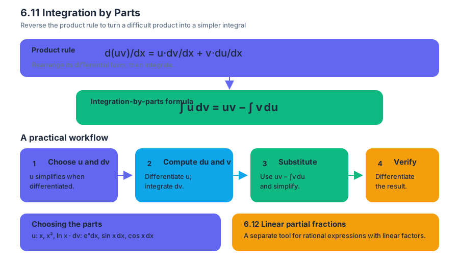
6.12 Integrating Using Linear Partial Fractions (BC only)
Key concepts: Linear partial fractions (BC only) · Decomposing rational functions into sums of ratios with linear, nonrepeating factors · Integrating the resulting partial-fraction terms · Recognizing integrands that are factors of a chain-rule derivative · Using u-substitution as a basic integration technique · Determining indefinite integrals of rational functions
How to decompose a rational function with distinct linear factors into partial fractions and integrate each piece as a logarithm.
6.12 Integrating Using Linear Partial Fractions (BC only)
A rational function whose denominator factors into distinct linear pieces can be rewritten as a sum of simple fractions, each a constant over one linear factor. Every such fraction integrates to a logarithm, so this page starts with that one-term rule and then builds the decomposition on top of it. The technique is BC only.
Recognizing reverse chain-rule structure
Integration methods often begin with pattern recognition. In
$$ \int \frac{A}{ax+b},dx, $$
the denominator $ax+b$ has derivative $a$, a constant factor already present in the numerator after adjustment. Set
$$ u=ax+b, \qquad du=a,dx. $$
Because $dx=\frac{du}{a}$,
$$ \int \frac{A}{ax+b},dx
\frac{A}{a}\int \frac{1}{u},du
\frac{A}{a}\ln|u|+C
\boxed{\frac{A}{a}\ln|ax+b|+C}. $$
For example,
$$ \int \frac{6}{3x-2},dx
2\ln|3x-2|+C. $$
This is a reverse chain-rule move: recognize the derivative of the inner linear expression, adjust by its constant factor, and obtain a logarithm.
Linear partial fractions
A rational function is a quotient of polynomials. When its denominator factors into distinct, nonrepeating linear factors, the rational function may be decomposed into a sum of simpler ratios. This is the central idea of linear partial fractions, identified by FUN-6.F and FUN-6.F.1.
Worked example: decomposition and integration
Decompose
$$ \frac{5x+1}{(x+1)(x+2)}. $$
Because the denominator has two distinct linear factors, write
$$ \frac{5x+1}{(x+1)(x+2)}
\frac{A}{x+1}+\frac{B}{x+2}. $$
Multiplying by $(x+1)(x+2)$ gives
$$ 5x+1=A(x+2)+B(x+1). $$
Expanding and matching coefficients,
$$ 5x+1=(A+B)x+(2A+B), $$
so
$$ A+B=5, \qquad 2A+B=1. $$
Subtracting the first equation from the second gives $A=-4$, and then $B=9$. Thus,
$$ \frac{5x+1}{(x+1)(x+2)}
-\frac{4}{x+1}+\frac{9}{x+2}. $$
Integrate term by term:
$$ \begin{aligned} \int \frac{5x+1}{(x+1)(x+2)},dx &= -4\int\frac{1}{x+1},dx + 9\int\frac{1}{x+2},dx\ &= \boxed{-4\ln|x+1|+9\ln|x+2|+C}. \end{aligned} $$
Each term uses the linear-denominator rule with $a=1$. If the denominator were $4x-3$, the corresponding term would integrate as
$$ \int\frac{A}{4x-3},dx
\frac{A}{4}\ln|4x-3|+C. $$
The two recognition patterns
The methods can be distinguished by the structure of the integrand:
| Integrand structure | Recognition cue | Main move |
|---|---|---|
| Product such as $x e^x$ | Reverse product rule | $\int u,dv=uv-\int v,du$ |
| Rational function with distinct linear factors | Split the denominator into linear pieces | Partial-fraction decomposition |
| Ratio with a linear denominator | Numerator is related to the denominator’s derivative | Reverse chain rule and logarithm |
For FUN-6.F, linear partial fractions are used to determine indefinite or definite integrals of rational functions once the denominator has been factored into distinct linear factors. The associated suggested skill is 1.E — Apply appropriate mathematical rules or procedures, with and without technology.
Retrieval check: For
$$ \int \frac{7}{5x+1},dx, $$
identify the substitution and the coefficient multiplying the logarithm. Then decide whether
$$ \int x\cos x,dx $$
is better suited to substitution or integration by parts. The answers are $u=5x+1$, coefficient $\frac{7}{5}$, and integration by parts.
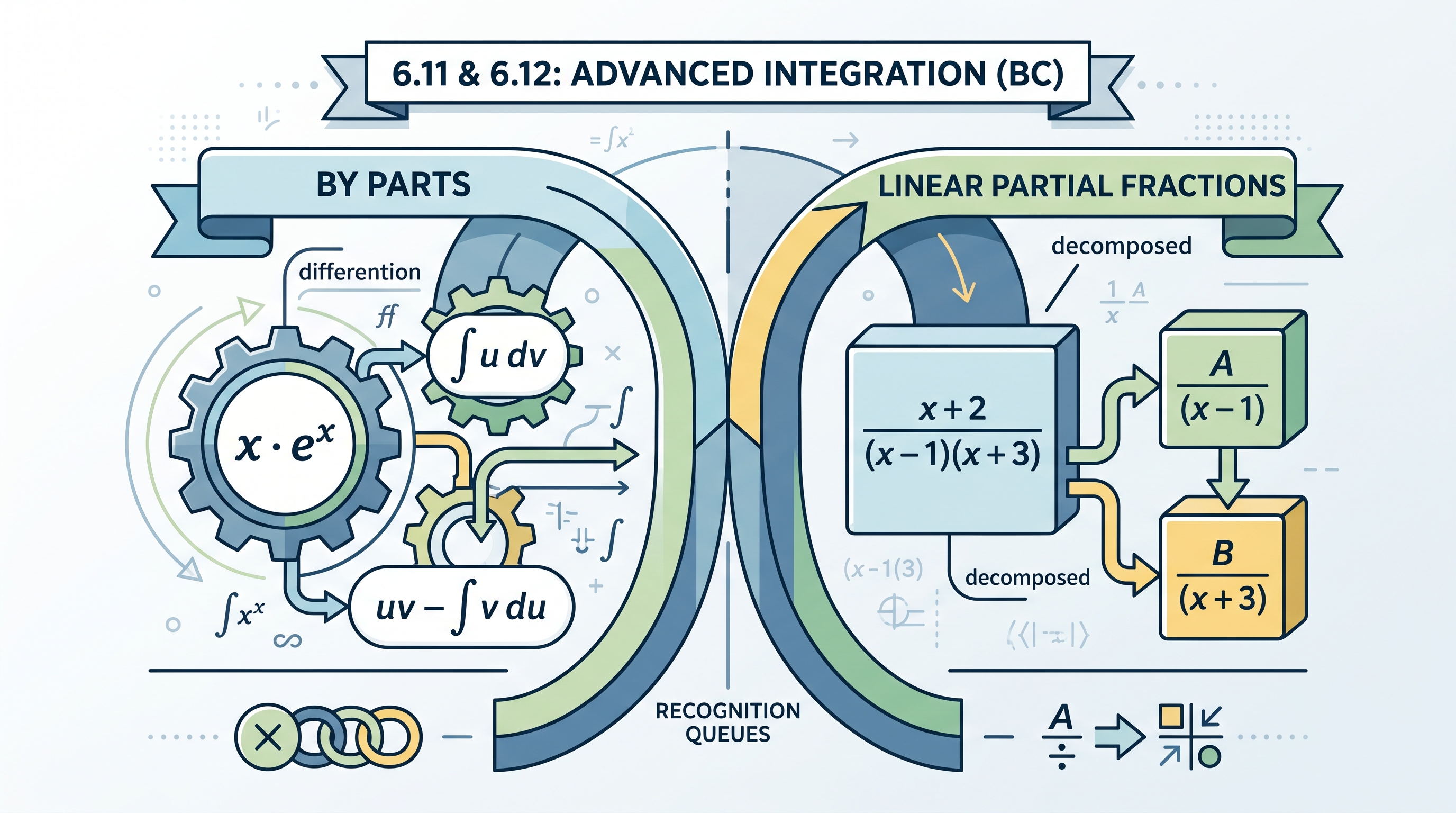
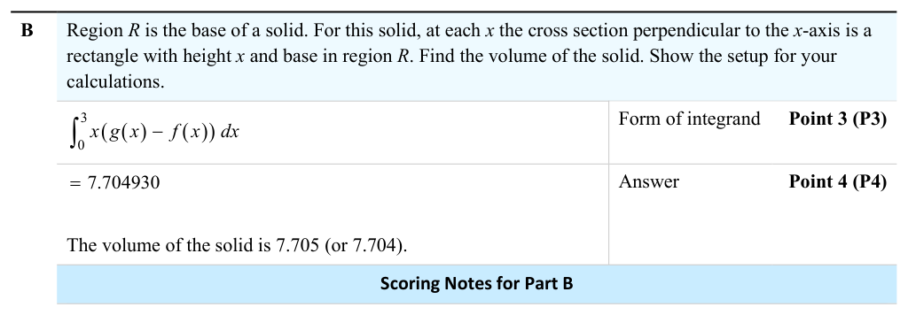
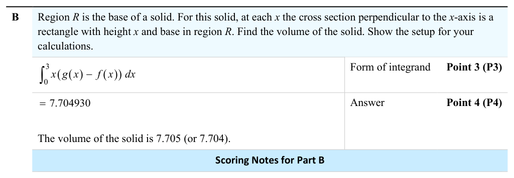
6.13 Evaluating Improper Integrals (BC only)
Key concepts: Evaluating improper integrals (BC only)
How to evaluate improper integrals by replacing an infinite endpoint or a singularity with a limit, and how to decide convergence or divergence.
6.13 Evaluating Improper Integrals (BC only)
An improper integral is a definite integral whose interval is infinite or whose integrand becomes unbounded within the interval. It is not evaluated by simply substituting an infinite endpoint or a forbidden input; instead, a limit determines whether the accumulated quantity approaches a finite value.
Improper integrals: replace the problem with a limit
For an infinite interval,
$$ \int_a^\infty f(x),dx
\lim_{b\to\infty}\int_a^b f(x),dx. $$
For an integrand that is undefined or unbounded at an endpoint,
$$ \int_a^c f(x),dx
\lim_{b\to c^-}\int_a^b f(x),dx. $$
If the limit exists as a finite number, the integral converges. If the limit does not exist or grows without bound, the integral diverges. This is the BC-only focus of Topic 6.13 Evaluating Improper Integrals, associated with LIM-6 and Skill 1.E: Apply appropriate mathematical rules or procedures, with and without technology.
Worked example. Determine whether
$$ \int_1^\infty \frac{1}{x^2},dx $$
converges.
First replace $\infty$ with a variable endpoint:
$$ \int_1^\infty \frac{1}{x^2},dx
\lim_{b\to\infty}\int_1^b x^{-2},dx. $$
Using the power rule,
$$ \int_1^b x^{-2},dx
\left[-x^{-1}\right]_1^b
-\frac{1}{b}+1. $$
Therefore,
$$ \lim_{b\to\infty}\left(1-\frac{1}{b}\right)=1. $$
The integral converges to $1$. The infinite interval does not automatically make an integral infinite; the function’s decay determines the result.
Contrast: a divergent integral. The same steps applied to $\int_1^\infty\frac{1}{x},dx$ give $\lim_{b\to\infty}\left[\ln x\right]1^b=\lim{b\to\infty}\ln b$, which grows without bound, so this integral diverges. Both $\frac{1}{x}$ and $\frac{1}{x^2}$ approach $0$, but only $\frac{1}{x^2}$ decays fast enough for the accumulated area to stay finite.
Endpoint warning. If the integrand is unbounded at an interior point $c$, split the integral:
$$ \int_a^b f(x),dx
\int_a^c f(x),dx+\int_c^b f(x),dx, $$
and evaluate both pieces as separate one-sided limits. The entire integral converges only if both pieces converge.
Retrieval check: Write $\int_0^1\frac{1}{\sqrt{x}},dx$ as a limit and decide whether it converges. The integrand is unbounded at $x=0$, so $\int_0^1 x^{-1/2},dx=\lim_{a\to0^+}\left[2\sqrt{x}\right]a^1=\lim{a\to0^+}\left(2-2\sqrt{a}\right)=2$. The integral converges to $2$.
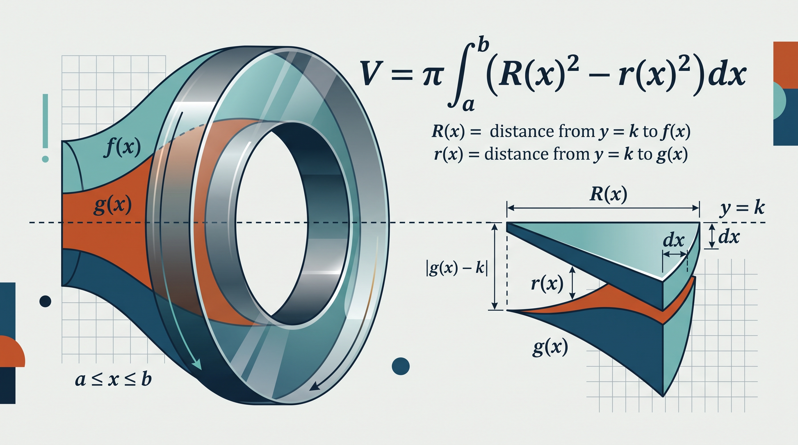
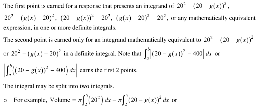
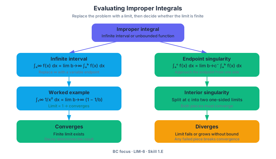
6.14 Selecting Techniques for Antidifferentiation
Key concepts: Selecting appropriate techniques for antidifferentiation · Classifying an expression to identify the applicable mathematical rule or procedure (Skill 1.C) · Using partial fractions for antidifferentiation (BC only) · Using the washer method to find volume when revolving a region · Revolving regions around axes other than the usual coordinate axes · Finding distance traveled through antidifferentiation · Applying rules and procedures for antidifferentiation in Personal Progress Checks 6–8
How to classify an integrand and pick the matching antidifferentiation technique, with applications to distance traveled and washer volumes.
6.14 Selecting Techniques for Antidifferentiation
By this point the unit has built a full toolkit: basic rules, substitution, long division, completing the square and, for BC, integration by parts and partial fractions. On an exam nobody tells you which one to use. This topic is about reading the structure of an integrand and choosing the technique that fits it.
Selecting an antidifferentiation technique
Topic 6.14 Selecting Techniques for Antidifferentiation belongs to FUN-6 and emphasizes Skill 1.C: Identify an appropriate mathematical rule or procedure based on the classification of a given expression. The central question is not “Which formula have I just practiced?” but “What structural feature does this integrand have?”
Use the following classification pipeline:
| Form of the integrand | First procedure to consider |
|---|---|
| Sum of powers, constants, or basic functions | Basic antiderivative rules |
| A composite expression multiplied by its inner derivative | Substitution |
| A product such as polynomial times exponential or logarithmic function | Integration by parts |
| A rational function with a denominator that factors into linear terms | Partial fractions, BC only |
| A rational function with numerator degree at least the denominator degree | Long division first |
| A quadratic denominator | Completing the square or a related standard form |
| A definite integral with a singularity or infinite endpoint | Improper-integral limit |
For example,
$$ \int 2x\cos(x^2),dx $$
is classified as a composite-function pattern: the inner function is $u=x^2$, and $du=2x,dx$. Thus,
$$ \int 2x\cos(x^2),dx
\sin(x^2)+C. $$
By contrast,
$$ \int x e^x,dx $$
is a product pattern, so integration by parts is appropriate. For a BC-only rational example,
$$ \int \frac{1}{x^2-1},dx, $$
factor the denominator as $(x-1)(x+1)$ and use partial fractions before integrating.
Named misconception — “Any technique will work if I manipulate long enough.” A method can create unnecessary algebra or fail completely when the expression is misclassified. In Skill 1.C, the classification itself is part of the mathematics: identify the form, select the rule, then execute it accurately. Practice should therefore mix techniques rather than group identical integrals together.
Antidifferentiation in applications
Antidifferentiation also converts a rate into a total change. If velocity is $v(t)$, then displacement on $[a,b]$ is
$$ \int_a^b v(t),dt, $$
while distance traveled is
$$ \int_a^b |v(t)|,dt. $$
The absolute value matters because negative velocity indicates motion in the negative direction, not negative distance. Split the interval wherever $v(t)=0$ before evaluating the distance integral.
Worked application. Suppose
$$ v(t)=t-2 $$
for $0\le t\le4$. The particle changes direction at $t=2$. Its distance traveled is
$$ \int_0^2 (2-t),dt+\int_2^4(t-2),dt
2+2=4 $$
units. The signed displacement,
$$ \int_0^4(t-2),dt=0, $$
is different: the particle returns to its starting position.
Washer method and rotation around other axes
When a region is revolved, each thin slice becomes a cross-sectional disk or washer. For slices perpendicular to the axis of rotation,
$$ V=\pi\int_a^b\left(R(x)^2-r(x)^2\right),dx, $$
where $R$ is the outer radius and $r$ is the inner radius. A radius is always a distance to the axis, so revolving around $y=k$ requires expressions such as $|f(x)-k|$, not merely $f(x)$.
For example, revolving the region between $y=x$ and $y=x^2$ on $0\le x\le1$ around the horizontal line $y=2$ produces washers. The outer radius is $R(x)=2-x^2$, and the inner radius is $r(x)=2-x$, giving
$$ V=\pi\int_0^1\left[(2-x^2)^2-(2-x)^2\right],dx. $$
The same principle handles axes other than the coordinate axes: measure every radius from the stated axis, choose slices perpendicular to that axis, and split the integral if the outer and inner boundaries change.
Retrieval check. Classify each expression before integrating: $\int (3x^2+4),dx$, $\int 6x\sqrt{3x^2+1},dx$, and $\int \frac{x}{x^2+1},dx$. Which use basic rules, which use substitution, and why? For an improper integral, what must replace an infinite endpoint?
7.1 Modeling Situations with Differential Equations
Key concepts: Modeling situations with differential equations
How to translate a verbal description of a changing quantity into a differential equation, including the sign and units of the proportionality constant.
7.1 Modeling Situations with Differential Equations
A differential equation does not usually tell you a function directly; it tells you how the function must change. That makes it a compact model of growth, motion, cooling, population change, or any situation in which a quantity’s rate depends on other quantities.
Investigative question: If you know a quantity’s rate of change, how can you describe the quantity itself—and how can you prove that a proposed function really works?
From words to a differential equation
A differential equation is an equation involving an unknown function and one or more of its derivatives. To model a situation, translate the verbal description into relationships among quantities before attempting to solve anything.
| Verbal statement | Mathematical model |
|---|---|
| The rate of change of $y$ with respect to $t$ is proportional to $y$ | $\dfrac{dy}{dt}=ky$ |
| The rate of change of $y$ is proportional to the amount of $y$ and decreases as $y$ approaches a capacity | $\dfrac{dy}{dt}=ky\left(1-\dfrac{y}{M}\right)$ |
| The rate of change of position is velocity | $\dfrac{ds}{dt}=v(t)$ |
In these models, $k$ is a constant of proportionality, $t$ is often time, and $M$ may represent a limiting capacity. The equation $\dfrac{dy}{dt}=ky$ says that the relative rate of change is constant: a larger amount of $y$ produces a larger absolute change.
Worked modeling example. A population $P$ grows at a rate proportional to its current size. Because “rate of change” means a derivative and “with respect to time” means differentiation by $t$, the model is
$$ \frac{dP}{dt}=kP. $$
If the population decreases rather than grows, then $k<0$. If it grows, then $k>0$. The sign and units matter: if $P$ is measured in organisms and $t$ in hours, then $k$ has units of hours$^{-1}$, so that $kP$ has units of organisms per hour.
Writing the equation is the modeling step. Checking that a proposed function actually satisfies it is the work of Topic 7.2.
AP skills in action
Topic 7.1 develops Skill 2.C: Use appropriate mathematical procedures by translating verbal relationships into differential equations and using antidifferentiation appropriately. Topic 7.2 develops Skill 3.G: Confirm that solutions are accurate and appropriate by differentiating a proposed function and checking the original equation.
Retrieval check: A cup of coffee at temperature $T$ cools at a rate proportional to the difference between $T$ and the room temperature of $20$ °C. Write a differential equation for $T$. One model is $\dfrac{dT}{dt}=k(T-20)$ with $k<0$: the derivative is the rate, $T-20$ is the quantity the rate is proportional to, and the negative constant makes a cup that is hotter than the room cool down.
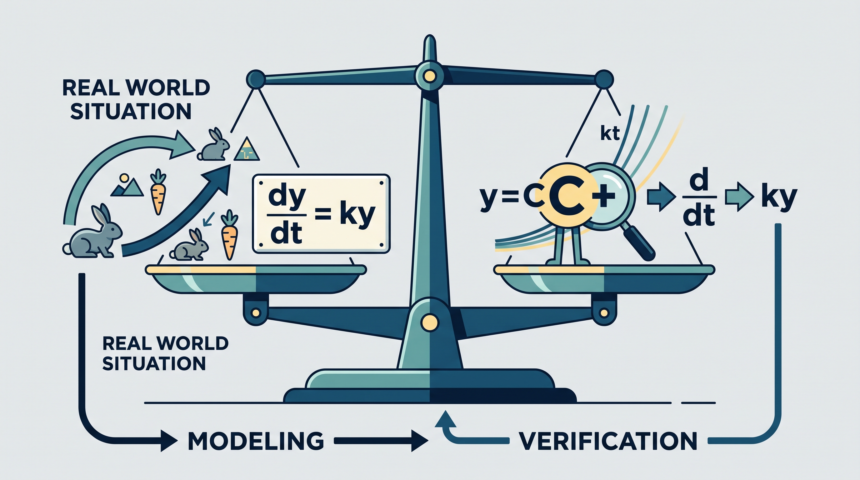
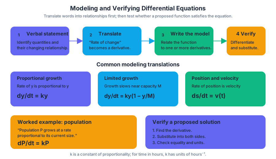
7.2 Verifying Solutions for Differential Equations
Key concepts: Verifying solutions to differential equations · Using derivatives to verify solutions · Estimating solutions with slope fields · Interpreting slope fields as graphical representations of differential equations · Using antidifferentiation to find general solutions · Recognizing that differential equations may have infinitely many solutions · Exponential solutions to equations of the form dy/dt = ky
How to verify a proposed solution by differentiating and substituting, and why one differential equation has a whole family of solutions until an initial condition selects one.
7.2 Verifying Solutions for Differential Equations
Topic 7.1 turned a verbal description into a differential equation. The next question is whether a proposed function really satisfies that equation. Answering it needs no solving technique: differentiate, substitute, and check that the two sides agree. The same check shows that one differential equation can be satisfied by a whole family of functions.
Investigative question: If you know a quantity’s rate of change, how can you describe the quantity itself—and how can you prove that a proposed function really works?
Verifying a proposed solution
The learning objective FUN-7.B: Verify solutions to differential equations requires checking, not guessing. The essential knowledge is FUN-7.B.1: Derivatives can be used to verify that a function is a solution to a given differential equation.
To verify a proposed function, differentiate it as many times as the differential equation requires, substitute the derivatives and the function into the equation, and determine whether the resulting statement is true on the relevant domain.
Worked verification. Test whether
$$ y=4e^{3t} $$
is a solution of
$$ \frac{dy}{dt}=3y. $$
Differentiate:
$$ \frac{dy}{dt}=12e^{3t}. $$
Now substitute $y=4e^{3t}$ into the right-hand side:
$$ 3y=3(4e^{3t})=12e^{3t}. $$
Because $\dfrac{dy}{dt}=3y$, the proposed function is a solution.
For a second-order equation, compute the second derivative too. For example, if the equation contains $\dfrac{d^2y}{dt^2}$, checking only the first derivative is incomplete.
Why one equation can have infinitely many solutions
The essential knowledge FUN-7.B.2: There may be infinitely many solutions to a differential equation is visible in the equation $\dfrac{dy}{dt}=ky$. Antidifferentiation gives
$$ \frac{1}{y},dy=k,dt, $$
so
$$ \ln|y|=kt+C. $$
Rewriting the constant produces the general solution
$$ y=Ce^{kt}. $$
Every value of $C$ gives a different solution. Thus $y=2e^{kt}$, $y=10e^{kt}$, and $y=-e^{kt}$ all satisfy the same differential equation when their domains are appropriate. An initial condition, such as $y(0)=6$, selects one particular solution:
$$ 6=Ce^0 \quad\Longrightarrow\quad C=6, $$
so $y=6e^{kt}$.
Slope fields as a first visual estimate
A slope field is a graphical representation of a differential equation on a finite set of points in the plane. At each point $(t,y)$, a short line segment shows the slope required by the differential equation.
For $\dfrac{dy}{dt}=ky$, points with the same $y$-value have the same slope because the right side depends only on $y$. A solution curve can be estimated by tracing a smooth path whose tangent follows the small segments. The exact sketching and reasoning procedures belong to Topics 7.3 and 7.4; here, the key connection is that the differential equation supplies local direction while the solution supplies the global curve.
AP skills in action
Topic 7.2 develops Skill 3.G: Confirm that solutions are accurate and appropriate. In written work, show the derivative of the proposed function, substitute it and the function into the original equation, and state that the two sides agree on the relevant domain. Claiming that a function works, without that substitution, is not a verification.
Misconception check — “A differential equation has one answer.” A differential equation may describe a family of functions. Constants such as $C$ remain until an initial condition or other restriction identifies a particular member.
Retrieval check: Does $y=7e^{-2t}$ satisfy $\dfrac{dy}{dt}=-2y$? Differentiate: $\dfrac{dy}{dt}=-14e^{-2t}$. Since $-2y=-14e^{-2t}$, it does.
7.3 Sketching Slope Fields
Key concepts: Slope fields · Sketching slope fields · Matching equations to slope fields · Translating mathematical information between representations · Rewriting verbal statements mathematically
How to sketch a slope field by evaluating the differential equation at chosen points, and how to match a field to its equation using zero slopes and sign changes.
7.3 Sketching Slope Fields
A differential equation can be read as a rule for drawing tiny tangent lines across the entire coordinate plane. A slope field is a collection of short line segments where each segment at $(x,y)$ has slope equal to the value prescribed by the differential equation.
For an equation such as
$$\frac{dy}{dx}=x-y,$$
the segment located at $(2,1)$ has slope $2-1=1$, while the segment at $(2,4)$ has slope $2-4=-2$. The field does not yet show one particular solution; it shows the local direction that every solution must follow.
Reading the geometry of a slope field
To sketch a slope field, choose several representative points, evaluate the right-hand side, and draw a short segment with that slope. Horizontal segments correspond to slope $0$, upward segments to positive slopes, and downward segments to negative slopes. Equal slope values create visually aligned segments, which often reveal the equation’s structure more efficiently than plotting point by point.
For
$$\frac{dy}{dx}=y-2,$$
the slope depends only on $y$, not on $x$. Therefore every point on the same horizontal line has the same slope:
- below $y=2$, segments slope downward;
- on $y=2$, segments are horizontal;
- above $y=2$, segments slope upward.
A solution passing through a point must be tangent to the segments as it moves across the field.
Matching an equation to a slope field
Matching requires looking for structural clues rather than estimating every segment. Ask three questions:
- Does the slope change horizontally? If the segments in each horizontal row look alike, the equation may depend only on $y$.
- Where are the horizontal segments? These occur where $\frac{dy}{dx}=0$.
- How does the sign change? Compare the directions above and below a horizontal or vertical equilibrium line.
Suppose a field has horizontal segments along $y=2$, upward segments above $y=2$, and downward segments below $y=2$. The equation
$$\frac{dy}{dx}=y-2$$
matches that field. At $y=2$, the derivative is $0$; when $y>2$, it is positive; and when $y<2$, it is negative.
A crucial language distinction appears when translating verbal statements. “The signed difference between $y$ and $2$” can mean $y-2$, so the model is
$$\frac{dy}{dx}=k(y-2).$$
But “the distance between $y$ and $2$” is an unsigned quantity. Distance cannot be negative, so it must be represented by an absolute value:
$$\frac{dy}{dx}=k\lvert y-2\rvert.$$
If $k>0$, this second equation gives positive slopes both above and below $y=2$, with horizontal segments on $y=2$. Confusing distance with signed difference reverses the direction of the field below $y=2$.
Misconception check — “distance” always means subtraction.
The expression $y-2$ records direction: it is negative when $y$ lies below $2$. The expression $\lvert y-2\rvert$ records only separation. Translate the wording first; choose the algebra afterward.
Translating among representations
The same information may appear as an equation, a slope field, or a verbal statement:
| Representation | Evidence to extract |
|---|---|
| Equation $\frac{dy}{dx}=F(x,y)$ | Compute the slope at $(x,y)$ |
| Slope field | Observe sign, steepness, and horizontal segments |
| Verbal statement | Identify the changing quantity, independent variable, and signed or unsigned relationship |
For example, “the rate at which $y$ changes is proportional to the signed difference between $y$ and $2$” becomes $\frac{dy}{dx}=k(y-2)$. “The rate is proportional to the distance from $y=2$” becomes $\frac{dy}{dx}=k\lvert y-2\rvert$. In each case, the graphical test is immediate: locate $y=2$, then inspect the slopes on either side.
This work develops Mathematical Practice 2—Connecting Representations by moving between equations, slope fields, and verbal descriptions. It also uses Mathematical Practice 3—Justification when a conclusion is supported by slope signs or equilibrium lines, and Mathematical Practice 4—Communication and Notation when variables, derivatives, constants, and absolute values are written precisely.
Retrieval check
For $\frac{dy}{dx}=x-y$, compute the slopes at $(1,1)$, $(0,2)$ and $(3,1)$, and say where the horizontal segments lie. The slopes are $0$, $-2$ and $2$. Horizontal segments occur where $x-y=0$, along the line $y=x$; above that line the segments slope downward, and below it they slope upward.
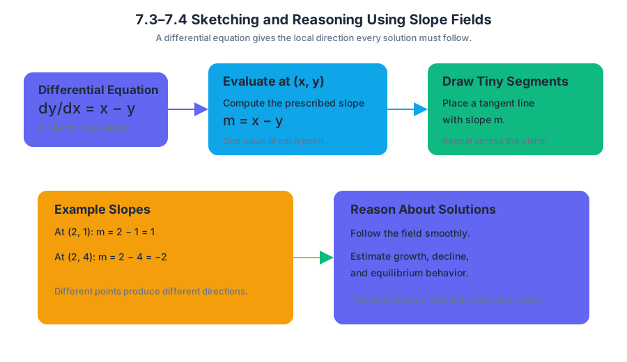
7.4 Reasoning Using Slope Fields
Key concepts: Slope fields · Reasoning using slope fields · Translating mathematical information between representations
How to read a slope field to predict where solutions rise or fall, how fast they change, and where equilibrium solutions lie, without solving the equation.
7.4 Reasoning Using Slope Fields
Topic 7.3 built a slope field by drawing, at each point, a short segment with the slope the differential equation prescribes. This page uses the finished field. Without solving the equation, the segments show where solutions rise or fall, how quickly they change, and which constant solutions never move. The running example is $\frac{dy}{dx}=y-2$: its segments are horizontal along $y=2$, tilt upward above that line and downward below it.
A solution passing through a point must be tangent to the segments as it moves across the field.
Reasoning from a slope field
A slope field supports qualitative predictions even when no explicit formula for $y$ is available. If the segments along a solution’s path are positive, the solution increases; if they are negative, it decreases. Segments that become progressively steeper indicate faster change, while segments that flatten indicate slower change.
For $\frac{dy}{dx}=y-2$, a solution beginning at $(0,3)$ initially increases because its slope is $1$. As it rises above $y=2$, the slope becomes even larger, so the curve bends upward and moves away from $y=2$. A solution beginning at $(0,1)$ initially decreases because its slope is $-1$; below $y=2$, the field continues directing it downward.
The line $y=2$ is an equilibrium solution because its derivative is always zero there. A solution that starts exactly on this line remains horizontal.
Every solution follows the same field, so a slope field describes a whole family of solutions at once; an initial point selects one of them. To sketch the solution through a given point, start there and draw a smooth curve, in both directions, that stays tangent to the nearby segments. Follow the flow of the field rather than joining segments end to end. For $\frac{dy}{dx}=y-2$, a curve that starts above $y=2$ stays above it, and one that starts below stays below.
This work develops Mathematical Practice 2—Connecting Representations by moving between equations, slope fields, and verbal descriptions. It also uses Mathematical Practice 3—Justification when a conclusion is supported by slope signs or equilibrium lines, and Mathematical Practice 4—Communication and Notation when variables, derivatives, constants, and absolute values are written precisely.
Retrieval check
For the equation
$$\frac{dy}{dx}=-(y+1),$$
identify the horizontal line of equilibrium, state whether slopes are positive or negative above that line, and predict the direction of a solution beginning at $(0,-3)$.
The equilibrium line is $y=-1$. Below it, $y+1<0$, so $-(y+1)>0$ and the slopes are positive. Thus a solution beginning at $(0,-3)$ initially increases.
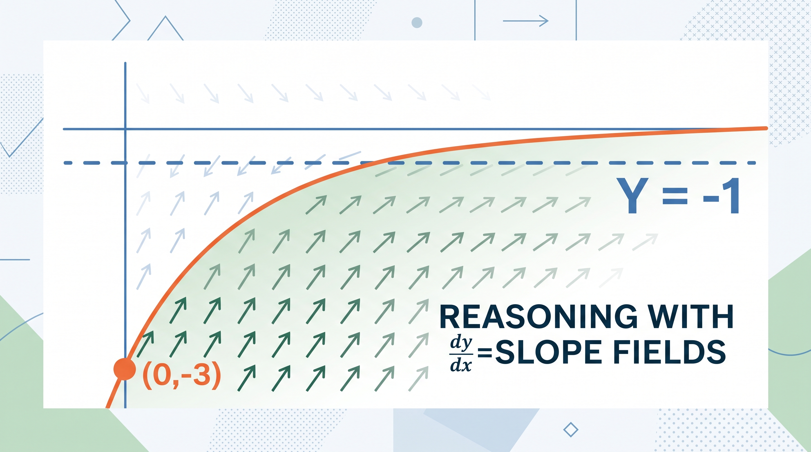
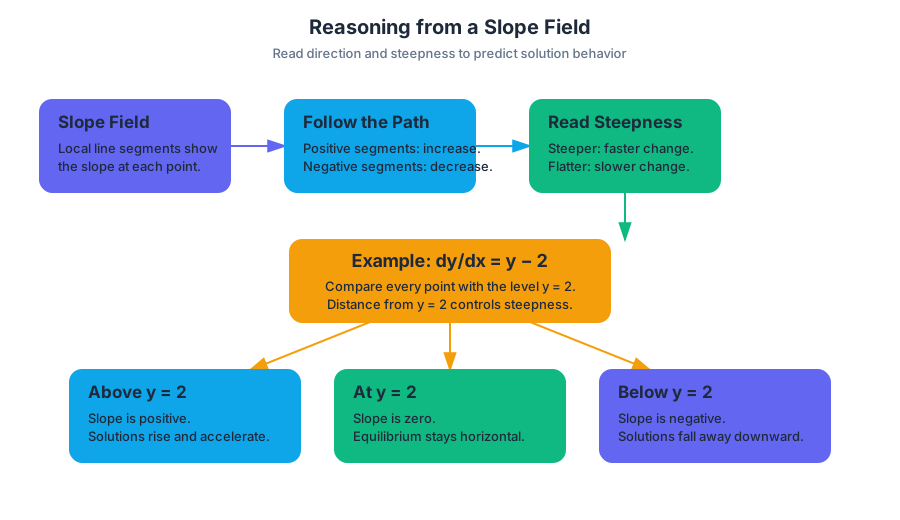
7.5 Approximating Solutions Using Euler’s Method (BC only)
Key concepts: Euler’s method for approximating solutions to differential equations · Estimating solutions to differential equations · Solving differential equations to determine functions and develop models · The relationship between differential equations and slope fields · Logistic growth models · Use of appropriate graphing techniques · Topic 7.5 is BC-only content · FUN-7.C.4: Euler’s method
How Euler’s method builds an approximate solution from repeated tangent-line steps, how step size affects accuracy, and how to apply it to a logistic model (BC only).
7.5 Approximating Solutions Using Euler’s Method (BC only)
A differential equation can describe a changing system even when no convenient formula for the system exists. Euler’s method follows the local slope repeatedly: start at a known point, use the differential equation to estimate the slope there, and step forward to create an approximate solution curve.
BC-only scope: Topic 7.5, Approximating Solutions Using Euler’s Method, is BC-only. Topic 7.6, Finding General Solutions Using Separation of Variables, is part of the differential-equation progression for both AB and BC. Logistic growth models are also BC-only content.
The governing enduring understanding is FUN-7: “Solving differential equations allows us to determine functions and develop models.” The related learning objective is FUN-7.C: “Estimate solutions to differential equations.” The essential knowledge statement FUN-7.C.4 specifies that Euler’s method approximates either a solution to a differential equation or a point on a solution curve. The suggested skill is 1.E: Apply appropriate mathematical rules or procedures, with and without technology.
Euler’s method: turning slope into a path
Suppose a population satisfies
$$ \frac{dy}{dx}=f(x,y) $$
and the solution passes through the known point $(x_0,y_0)$. At that point, the differential equation gives the slope $f(x_0,y_0)$. For a step size $h$, Euler’s method estimates the next point by
$$ x_{n+1}=x_n+h, $$
$$ y_{n+1}=y_n+h f(x_n,y_n). $$
The essential idea is geometric: replace the unknown curve over a short interval by the tangent-line segment determined by the current point and current slope.
For example, approximate the solution to
$$ \frac{dy}{dx}=x+y $$
that passes through $(0,1)$ using step size $h=0.2$.
At $(x_0,y_0)=(0,1)$, the slope is
$$ f(0,1)=0+1=1. $$
Therefore,
$$ y_1=1+0.2(1)=1.2, \qquad x_1=0.2. $$
At $(0.2,1.2)$,
$$ f(0.2,1.2)=0.2+1.2=1.4, $$
so
$$ y_2=1.2+0.2(1.4)=1.48, \qquad x_2=0.4. $$
At $(0.4,1.48)$,
$$ f(0.4,1.48)=1.88, $$
and hence
$$ y_3=1.48+0.2(1.88)=1.856, \qquad x_3=0.6. $$
Thus the Euler estimate for $y(0.6)$ is approximately $1.856$.
The calculation uses the current point to determine the current slope. A frequent error is to use the new point $(x_{n+1},y_{n+1})$ inside $f(x,y)$ before that point has been computed. Another is to forget the factor $h$; the vertical change is not merely the slope, but
$$ \Delta y\approx h\cdot \text{slope}. $$
Graphing and judging an Euler approximation
A useful graphing procedure is:
- Plot the initial point $(x_0,y_0)$.
- Calculate the slope from the differential equation at that point.
- Plot the next Euler point using the horizontal step $h$ and vertical change $h f(x_n,y_n)$.
- Repeat the process for the required interval.
- Connect consecutive points with short line segments, recognizing that the result is an approximation rather than the exact solution.
- If technology supplies a direction field, compare the Euler segments with the small slope marks at each point.
- Repeat with a smaller step size and compare the resulting paths.
A smaller step size usually produces a closer approximation because each line segment follows the changing slope for a shorter distance. However, “smaller” does not mean “exact”: Euler’s method still accumulates approximation error. If the curve bends strongly, a large step can jump noticeably away from the actual solution.
Euler’s method is often applied to population models. The logistic model below is a standard BC example: read its behavior from the equation first, then estimate values with Euler steps.
Logistic growth: limited resources create equilibria
A logistic model describes growth that slows as a population approaches a carrying capacity $K$:
$$ \frac{dP}{dt}=rP\left(1-\frac{P}{K}\right), $$
where $P$ is population, $r>0$ is the intrinsic growth constant, and $K>0$ is the carrying capacity.
The equilibrium solutions are
$$ P=0 \qquad\text{and}\qquad P=K. $$
If $0<P<K$, then $dP/dt>0$, so the population increases. If $P>K$, then $dP/dt<0$, so the population decreases toward $K$. The growth rate is greatest when $P=K/2$; near $0$ and near $K$, growth is slower.
For a BC-only Euler estimate, let
$$ \frac{dP}{dt}=0.4P\left(1-\frac{P}{1000}\right), \qquad P(0)=200, $$
with step size $h=1$. At $t=0$,
$$ P'(0)=0.4(200)\left(1-\frac{200}{1000}\right)=64. $$
Thus,
$$ P(1)\approx 200+1(64)=264. $$
At $P=264$,
$$ P'\approx 0.4(264)\left(1-\frac{264}{1000}\right)=77.7216, $$
so
$$ P(2)\approx264+77.7216=341.7216. $$
The population rises because it is below $K=1000$, but the model predicts eventual leveling rather than unlimited exponential growth.
For logistic equations, the equilibrium misconception is especially important: $K$ is not the initial population and does not mean the population instantly becomes $K$. It is the long-term balance level predicted by the model. A graph should show solutions below $K$ moving upward and solutions above $K$ moving downward.
Retrieval check
For
$$ \frac{dy}{dx}=x-y, \qquad y(0)=2, $$
with $h=0.5$, the first Euler estimate is
$$ y(0.5)\approx 2+0.5(0-2)=1. $$
Explain why the next slope must be evaluated at $(0.5,1)$, not at $(0,2)$, and identify the two equilibrium solutions of the logistic model
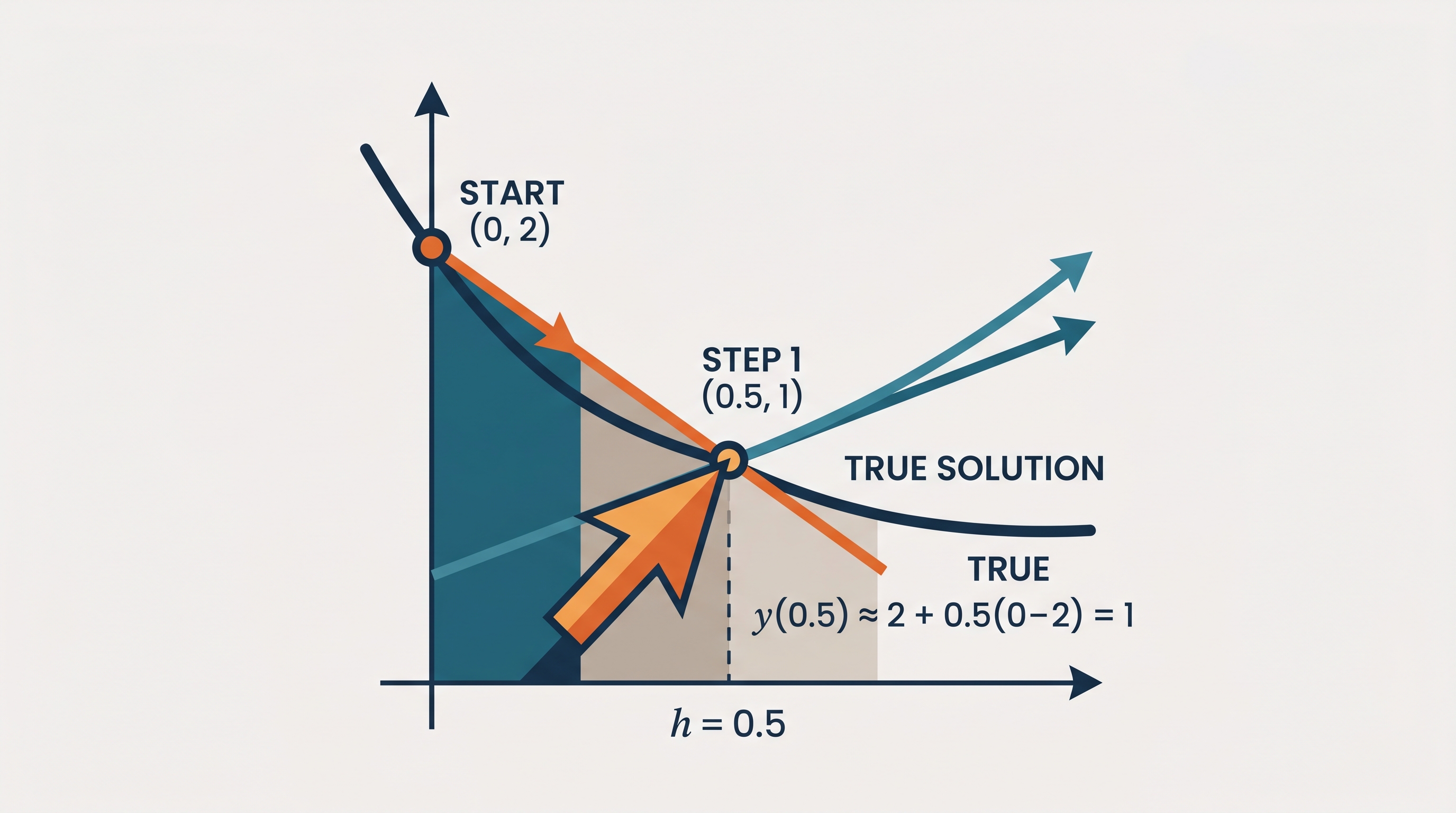
7.6 Finding General Solutions Using Separation of Variables
Key concepts: Solving differential equations to determine functions and develop models · Separation of variables for finding general solutions · Topic 7.6 involves finding general solutions
How to find the general solution of a separable differential equation by separating the variables and integrating both sides, without losing constant solutions.
7.6 Finding General Solutions Using Separation of Variables
Euler’s method (Topic 7.5) only approximates a solution, one step at a time. When the right-hand side of a differential equation factors into an $x$-part times a $y$-part, antidifferentiation gives the whole family of solutions at once. This topic is assessed on both AP Calculus AB and BC. The diagram below sets the numerical and symbolic approaches side by side.
Separation of variables: finding a general solution
Separation of variables solves a differential equation by placing all expressions involving $y$ with $dy$ and all expressions involving $x$ with $dx$. For a separable equation
$$ \frac{dy}{dx}=g(x)h(y), $$
rewrite it as
$$ \frac{1}{h(y)},dy=g(x),dx, $$
then integrate both sides.
Consider
$$ \frac{dy}{dx}=3xy. $$
For $y\neq 0$, separate:
$$ \frac{1}{y},dy=3x,dx. $$
Integrating gives
$$ \ln|y|=\frac{3}{2}x^2+C. $$
Exponentiating and absorbing the sign into the arbitrary constant produces the general solution
$$ y=Ce^{\frac{3}{2}x^2}. $$
The constant solution $y=0$ must also be recognized; it was lost temporarily when dividing by $y$. This is the division-by-a-variable misconception: algebraic division can remove an equilibrium solution, so check for it separately.
Not every equation separates. The right side of $\frac{dy}{dx}=x+y$ cannot be written as a product $g(x)h(y)$, so the method does not apply, while $\frac{dy}{dx}=\frac{x}{y}$ separates at once as $y,dy=x,dx$. Add the constant $C$ when you integrate, before solving for $y$; one constant is enough, because the constants from the two sides combine into one.
Retrieval check: Find the general solution of $\frac{dy}{dx}=\frac{x}{y}$. Separating gives $y,dy=x,dx$, and integrating gives $\frac{y^2}{2}=\frac{x^2}{2}+C$, so $y^2=x^2+C$ after renaming the constant. As a check, differentiating implicitly gives $2y\frac{dy}{dx}=2x$, which is the original equation.
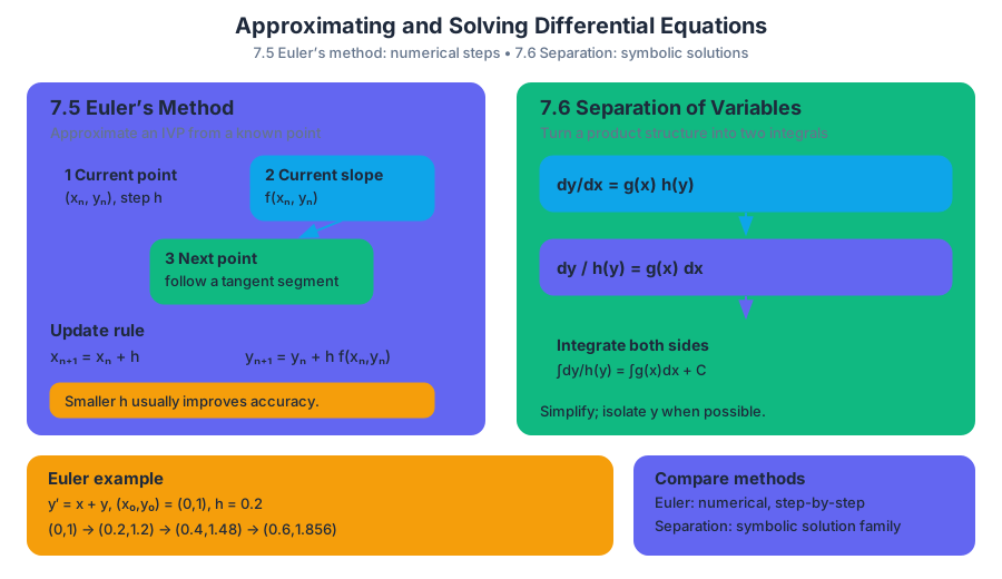
7.7 Finding Particular Solutions Using Initial Conditions and Separation of Variables
Key concepts: Solving differential equations to determine functions and develop models · Finding particular solutions using initial conditions · Separation of variables · Using integration to solve differential equations · Using initial conditions to determine the constant of integration
How to find the particular solution of a separable differential equation by integrating both sides and using an initial condition to determine the constant.
7.7 Finding Particular Solutions Using Initial Conditions and Separation of Variables
A differential equation becomes a model when its rate rule is paired with enough information to identify one specific function. The decisive move is often simple: separate the variables, integrate both sides, use an initial condition, and rearrange.
Enduring Understanding FUN-7: Solving differential equations allows us to determine functions and develop models.
From a rate rule to one particular function
A solution to a differential equation is a function that makes the equation true when its derivatives are substituted into it. For example, if $y(t)=50e^{0.2t}$, then $$ \frac{dy}{dt}=10e^{0.2t}=0.2\left(50e^{0.2t}\right)=0.2y. $$ Therefore, $y(t)=50e^{0.2t}$ is a solution of $\frac{dy}{dt}=0.2y$.
A differential equation usually has a family of solutions. The constant of integration distinguishes one member of that family from another. An initial condition, such as $y(0)=50$, identifies the particular solution passing through the specified point.
The separable-equation pipeline
For a separable differential equation, place all expressions involving the dependent variable on one side and all expressions involving the independent variable on the other:
$$ \frac{dy}{dt}=g(t)h(y) \quad\Longrightarrow\quad \frac{1}{h(y)},dy=g(t),dt. $$
Then integrate both sides, include the constant of integration, apply the initial condition, and solve for the desired function.
Worked example: a changing quantity with an initial measurement
Suppose a quantity $P$ satisfies $$ \frac{dP}{dt}=\frac{3t}{P}, \qquad P(1)=2. $$ The initial condition says that when $t=1$, the quantity has value $P=2$.
Step 1: Separate the variables. $$ P,dP=3t,dt $$
Step 2: Integrate both sides. $$ \int P,dP=\int 3t,dt $$ $$ \frac{P^2}{2}=\frac{3t^2}{2}+C. $$
Step 3: Use the initial condition to determine $C$. Substitute $P=2$ and $t=1$: $$ \frac{2^2}{2}=\frac{3(1)^2}{2}+C $$ $$ 2=\frac{3}{2}+C, \qquad C=\frac12. $$
Step 4: Rearrange to obtain the particular solution. $$ \frac{P^2}{2}=\frac{3t^2}{2}+\frac12 $$ $$ P^2=3t^2+1. $$ Because the initial value is positive, choose the positive branch: $$ \boxed{P(t)=\sqrt{3t^2+1}}. $$
The sign choice matters. Both $P=\sqrt{3t^2+1}$ and $P=-\sqrt{3t^2+1}$ satisfy the squared equation, but only the positive function satisfies $P(1)=2$.
The pipeline works the same way when the rate is proportional to the amount. For $\frac{dy}{dt}=ky$, separating gives $\frac{1}{y},dy=k,dt$, integrating gives $\ln|y|=kt+C$, and solving for $y$ gives the family $y=Ce^{kt}$. Topic 7.8 studies this exponential model in detail; here it is one more family from which an initial condition selects a single member.
AP skills in this topic
This work develops 1.E — Apply appropriate mathematical rules or procedures, with and without technology: separation, antidifferentiation, logarithm rules, constant selection, and algebraic rearrangement must remain visible. It also exercises the representation and modeling processes associated with [2.C], [3.G], and [4.D] by translating among equations, conditions, graphs, context, and notation.
Misconception check
“The constant of integration can be ignored because the initial condition supplies the missing information.” The initial condition does not replace $C$; it determines $C$. Omitting $C$ before applying the condition usually eliminates the entire family of possible solutions.
Retrieval check: For $$ \frac{dy}{dt}=3y, \qquad y(2)=10, $$ identify the model type and find the particular solution. The equation has exponential form, so $y=Ce^{3t}$. Since $10=Ce^6$, the answer is $$ \boxed{y(t)=10e^{3(t-2)}}. $$
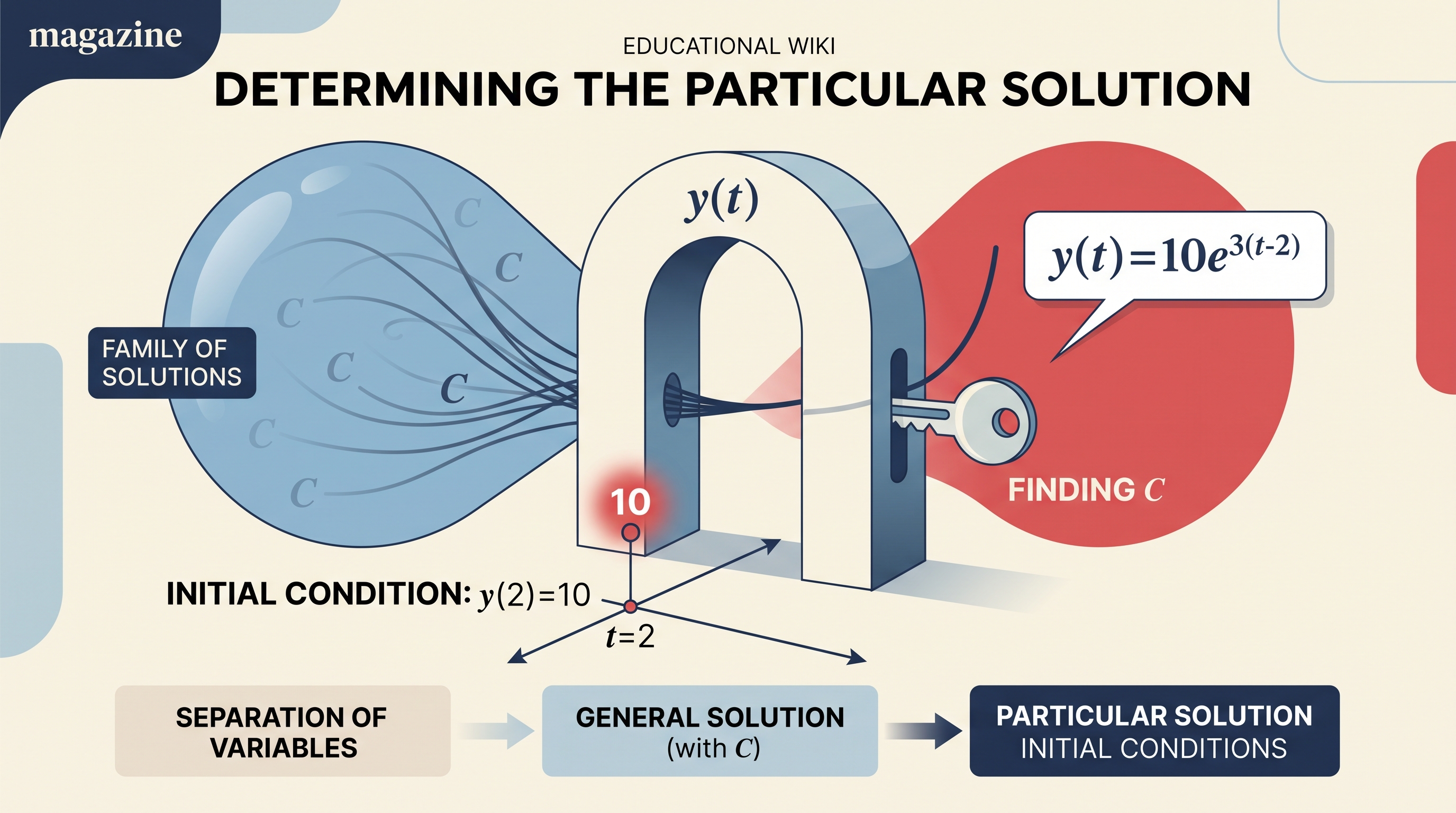
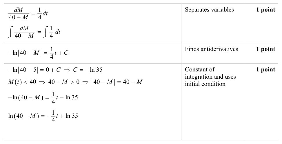
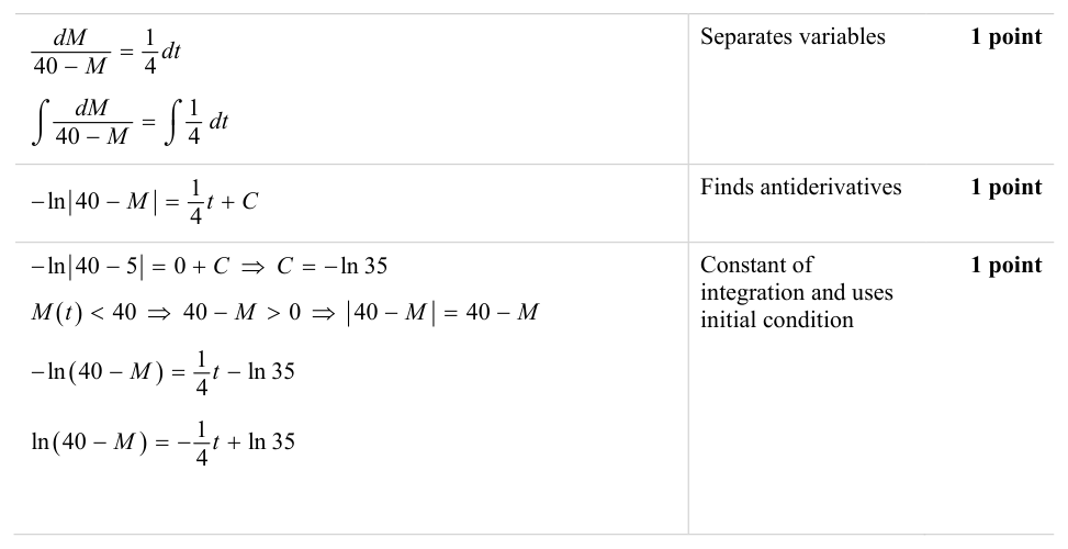
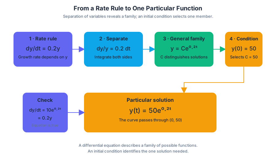
7.8 Exponential Models with Differential Equations
Key concepts: Solving differential equations to determine functions and develop models · Recognizing differential-equation forms that produce exponential models · Recognizing differential-equation forms that produce logistic models · Interpreting mathematical solutions in context · Exponential growth and decay models · Logistic models and carrying capacity
Why a rate proportional to the current amount gives the exponential model y = Ce^(kt), how to fit it to an initial value in context, and how it differs from logistic structure.
7.8 Exponential Models with Differential Equations
Topic 7.7 showed how separation of variables and an initial condition produce one particular solution. One differential equation appears so often in applications that its solution is worth recognizing on sight: when a quantity changes at a rate proportional to its current amount, the solution is always an exponential function. This page derives that model and applies it in context.
Enduring Understanding FUN-7: Solving differential equations allows us to determine functions and develop models.
Exponential models: recognize the form
The differential equation $$ \boxed{\frac{dy}{dt}=ky} $$ produces an exponential model because the rate of change is proportional to the current amount. Separating and integrating gives $$ \frac{1}{y},dy=k,dt \quad\Longrightarrow\quad \ln|y|=kt+C, $$ which rearranges to $$ y=Ce^{kt}. $$
If $k>0$, the model describes exponential growth; if $k<0$, it describes exponential decay. The constant $C$ is determined by an initial value. In context, $k$ has units of inverse time, while $y$ has the units of the modeled quantity.
Contextual example: population growth
A laboratory culture begins with $50$ organisms and grows at a rate proportional to its current population: $$ \frac{dP}{dt}=0.2P, \qquad P(0)=50. $$ The general solution is $P=Ce^{0.2t}$. Applying $P(0)=50$ gives $50=C$, so $$ \boxed{P(t)=50e^{0.2t}}. $$ After $5$ time units, $$ P(5)=50e^1\approx 135.914. $$ The model predicts approximately $136$ organisms, subject to the assumptions of continuous proportional growth.
Exponential versus logistic structure
A logistic differential equation includes a capacity-limiting factor: $$ \boxed{\frac{dP}{dt}=kP\left(1-\frac{P}{L}\right)}. $$ Here, $P$ is the current amount and $L$ is the carrying capacity. The product $P\left(1-\frac{P}{L}\right)$ distinguishes logistic growth from $\frac{dy}{dt}=ky$: growth depends both on the current amount and on the remaining capacity.
When $P$ approaches $L$, the factor $1-\frac{P}{L}$ approaches $0$, so the rate approaches $0$. Thus $L$ is the limiting population value, or carrying capacity. Recognizing this form is required for identifying logistic models; solving and analyzing logistic equations belong to the BC-only treatment of Topic 7.9.
Applications and representations
Differential-equation models can describe motion along a line as well as population change. If $s(t)$ is position, then $s'(t)=v(t)$ is velocity; a rule such as $\frac{dv}{dt}=kv$ models how velocity changes, while the initial position or velocity selects a particular motion. A strong solution connects the verbal situation, differential equation, graph or slope field, and final function.
This work develops 1.E — Apply appropriate mathematical rules or procedures, with and without technology: separation, antidifferentiation, logarithm rules, constant selection, and algebraic rearrangement must remain visible. It also exercises the representation and modeling processes associated with [2.C], [3.G], and [4.D] by translating among equations, conditions, graphs, context, and notation.
Retrieval check: A radioactive sample decays at a rate proportional to the amount present, with $k=-0.1$ per year and $A(0)=80$ grams. Write the model and find $A(10)$. The equation $\frac{dA}{dt}=-0.1A$ has exponential form, so $A(t)=80e^{-0.1t}$ and $A(10)=80e^{-1}\approx 29.4$ grams.
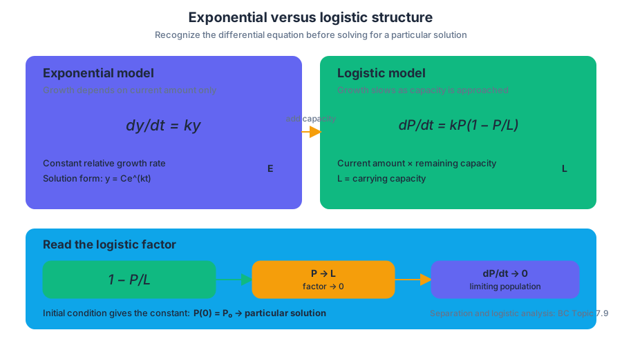
7.9 Logistic Models with Differential Equations (BC only)
Key concepts: Logistic models with differential equations · Exponential growth and decay · Solution curves of differential equations · General solutions and constants of integration · Particular solutions from initial conditions · Carrying capacity and asymptotic behavior · Interpreting the meaning of a differential equation · Developing mathematical models from differential equations · The equation dy/dt = ky · BC-only calculus content
A population can grow rapidly when resources are abundant, yet slow down as food, space, or energy becomes scarce. A logistic model captures both effects by making the growth rate depend on the population’s current size and its distance from a maximum sustainable level, called the carrying capacity.
7.9 Logistic Models with Differential Equations (BC only)
A population can grow rapidly when resources are abundant, yet slow down as food, space, or energy becomes scarce. A logistic model captures both effects by making the growth rate depend on the population’s current size and its distance from a maximum sustainable level, called the carrying capacity.
BC-only scope: Logistic models with differential equations are required for AP Calculus BC, not AP Calculus AB.
The governing enduring understanding is FUN-7: “Solving differential equations allows us to determine functions and develop models.” The learning objective is FUN-7.H: “Interpret the meaning of the logistic growth model in context. BC ONLY.” The essential knowledge identifiers for this topic are FUN-7.H.1, FUN-7.H.2, and FUN-7.H.3.
The logistic differential equation
Suppose $y(t)$ represents the size of a population at time $t$, and $a$ represents its carrying capacity. The statement “the rate of change is jointly proportional to the size of the quantity and the difference between the quantity and the carrying capacity” produces the logistic differential equation
$$ \frac{dy}{dt}=ky(a-y). $$
Here, $k$ is a proportionality constant. The factor $y$ means that a larger population can produce more offspring or otherwise generate more growth. The factor $a-y$ measures the remaining capacity: when $y$ is close to $a$, the population has little room for additional growth.
For a population with $0<y<a$ and $k>0$, both factors on the right side are positive, so $\frac{dy}{dt}>0$: the population increases. At $y=a$, the rate is zero, and when $y>a$, the rate becomes negative, pushing the population downward toward $a$.
The two equilibrium values are found by setting the rate equal to zero:
$$ ky(a-y)=0 \quad\Longrightarrow\quad y=0 \text{ or } y=a. $$
The value $y=a$ is the important long-term limit for a positive population below capacity.
Reading solution curves without solving
A solution curve is a function whose derivative satisfies the differential equation at every point in its domain. A direction field or graph of solution curves therefore shows how a population could evolve, even when no explicit formula for $y(t)$ has been found.
This is the key interpretation required by FUN-7.H.2: the logistic differential equation and initial conditions can be analyzed without solving the equation. The sign of $\frac{dy}{dt}$ reveals whether the curve rises or falls, while the size of $\left|\frac{dy}{dt}\right|$ indicates how steeply it changes.
Worked contextual example: a recovering fish population
A lake contains $20$ fish of a newly introduced species. The lake can support at most $100$ fish, and the population is modeled by
$$ \frac{dy}{dt}=0.002y(100-y), \qquad y(0)=20. $$
At the initial time,
$$ \frac{dy}{dt}
0.002(20)(100-20)
3.2. $$
Thus, the initial population is increasing at $3.2$ fish per unit of time. Because $0<20<100$, the population continues upward while remaining below the carrying capacity, although its growth eventually slows.
As $t\to\infty$, the population approaches
$$ \lim_{t\to\infty}y(t)=100. $$
The model does not predict unlimited growth. It predicts that the solution curve levels off toward $y=100$, so $100$ is the carrying capacity. This conclusion uses the logistic model and the initial condition, as required by FUN-7.H.3.
General solutions and particular solutions
A differential equation usually has infinitely many solutions. For example, the exponential equation
$$ \frac{dy}{dt}=ky $$
has the initial-value solution
$$ y=y_0e^{kt}, $$
but different values of $y_0$ produce different solution curves. More generally, solving introduces a constant of integration, so a general solution represents a whole family of functions.
An initial condition selects one member of that family. If a solution curve passes through the known point $(t_0,y_0)$, the corresponding function is called a particular solution. In a contextual problem, information such as an initial population, a measured value, or a known point on a graph supplies the condition needed to identify the relevant curve.
For logistic models, the initial condition also determines how the curve approaches the carrying capacity. A population beginning below $a$ generally rises toward $a$; a population beginning above $a$ generally falls toward $a$, assuming the parameters describe a meaningful population model.
Misconception check
Misconception: “The carrying capacity is the population’s current value.” The carrying capacity is instead the long-term limiting value built into the model. A population may start at $y(0)=20$, increase quickly, and still have carrying capacity $a=100$.
Skill connection — 3.F, “Explain the meaning of mathematical solutions in context.” A complete response should translate mathematics into the situation: identify what $y$ measures, state whether the quantity increases or decreases, interpret $\frac{dy}{dt}$ with units, and explain the meaning of the limiting value.
Retrieval check
For $\frac{dy}{dt}=0.01y(60-y)$ with $y(0)=10$, determine whether the quantity initially increases or decreases and state its expected long-term behavior.
Since
$$ \frac{dy}{dt}
0.01(10)(60-10)>0, $$
the quantity initially increases. Because the initial value lies below the carrying capacity, the solution is expected to approach $y=60$ as $t\to\infty$, rather than grow without bound.
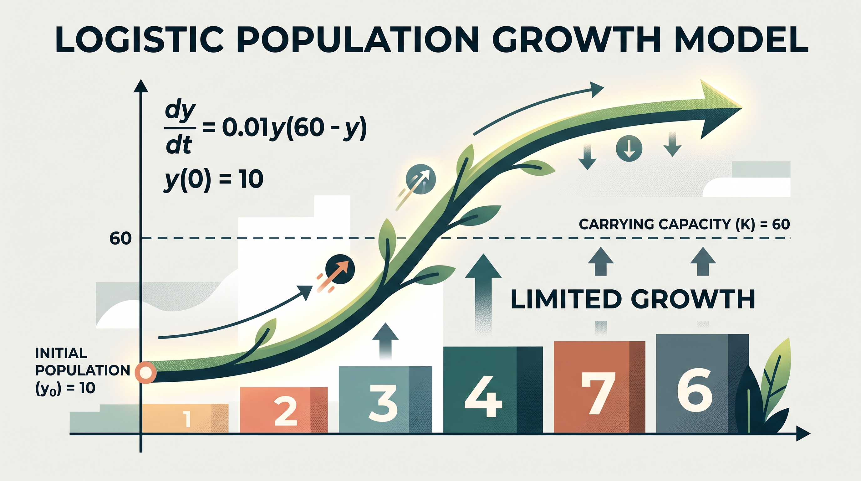
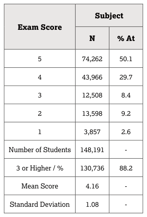
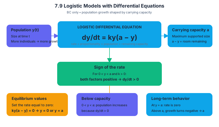
8.1 Finding the Average Value of a Function on an Interval
Key concepts: Average value of a continuous function on an interval · Distinguishing average value from average rate of change · Intermediate Value Theorem and function behavior on an interval
How to compute and interpret the average value of a function as its integral divided by the interval length, and why that is not the average rate of change.
8.1 Finding the Average Value of a Function on an Interval
A function’s average value is the height of a constant horizontal line that would produce the same accumulated area as the original function. That idea turns a changing quantity—temperature, flow rate, population density, or velocity—into one meaningful representative value.
Average value: “same area, constant height”
For a continuous function $f$ on the closed interval $[a,b]$, the average value is
$$ f_{\text{avg}}=\frac{1}{b-a}\int_a^b f(x),dx. $$
The definite integral gives the signed area under $f$, and dividing by the interval length $b-a$ converts that accumulated amount back into the units of $f$.
Geometric meaning: The rectangle with width $b-a$ and height $f_{\text{avg}}$ has exactly the same signed area as the region under $f$.
For example, let $f(x)=3x$ on $[1,4]$. Then
$$ f_{\text{avg}} =\frac{1}{4-1}\int_1^4 3x,dx =\frac{1}{3}\left[\frac{3x^2}{2}\right]_1^4 =\frac{1}{3}\cdot\frac{45}{2} =\frac{15}{2}. $$
Thus, the average value is $7.5$. The graph of $y=7.5$ forms a rectangle whose signed area from $x=1$ to $x=4$ equals the area under $y=3x$.
The same procedure works when the function is not algebraic. For $f(x)=x\sin x$ on $[0,\pi]$,
$$ f_{\text{avg}} =\frac{1}{\pi}\int_0^\pi x\sin x,dx. $$
Using integration by parts,
$$ \int x\sin x,dx=-x\cos x+\sin x, $$
so
$$ f_{\text{avg}} =\frac{1}{\pi}\left[-x\cos x+\sin x\right]_0^\pi =\frac{1}{\pi}(\pi)=1. $$
Average value is not average rate of change
The average rate of change measures how much the function’s output changes per unit of input:
$$ \frac{f(b)-f(a)}{b-a}. $$
The average value measures the mean height of the function:
$$ \frac{1}{b-a}\int_a^b f(x),dx. $$
These quantities answer different questions. For $f(x)=3x$ on $[1,4]$, the average rate of change is
$$ \frac{12-3}{4-1}=3, $$
whereas the average value is $7.5$. A common misconception is to use endpoint values to find average value; endpoint values determine average rate of change, not the accumulated mean.
Because $f$ is continuous, the Intermediate Value Theorem guarantees that $f$ takes every value between $f(a)$ and $f(b)$. The Average Value Theorem for integrals strengthens this idea: there is some $c\in[a,b]$ such that
$$ f(c)=f_{\text{avg}}. $$
The average height is therefore not merely an invented number; a continuous graph actually reaches it.
Topic 8.1 is paired with Skill 1.E: apply appropriate mathematical rules or procedures, with and without technology. For average value that means a correct setup $\frac{1}{b-a}\int_a^b f(x),dx$ on the stated interval, an exact evaluation or a calculator approximation of the integral, and an answer reported in the units of $f$ with an interpretation in context. When $f$ is known only from a table, estimate the integral with a Riemann or trapezoidal sum first, then divide by $b-a$.
Retrieval check: A continuous flow rate is $q(t)$ liters per minute on $[2,8]$. Write, but do not evaluate, the average flow rate and the total volume added. Then state which integral would determine displacement if $q$ were instead velocity.
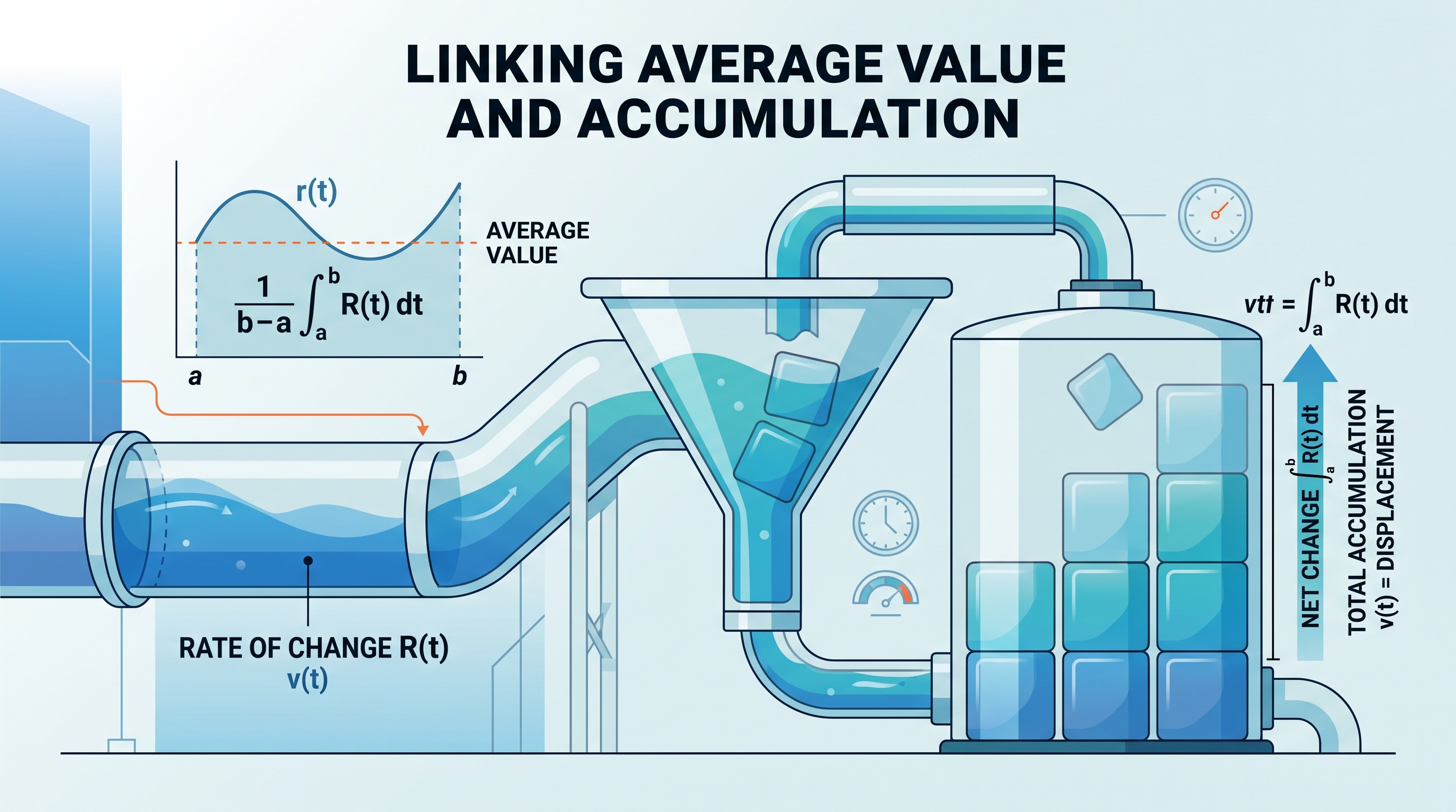
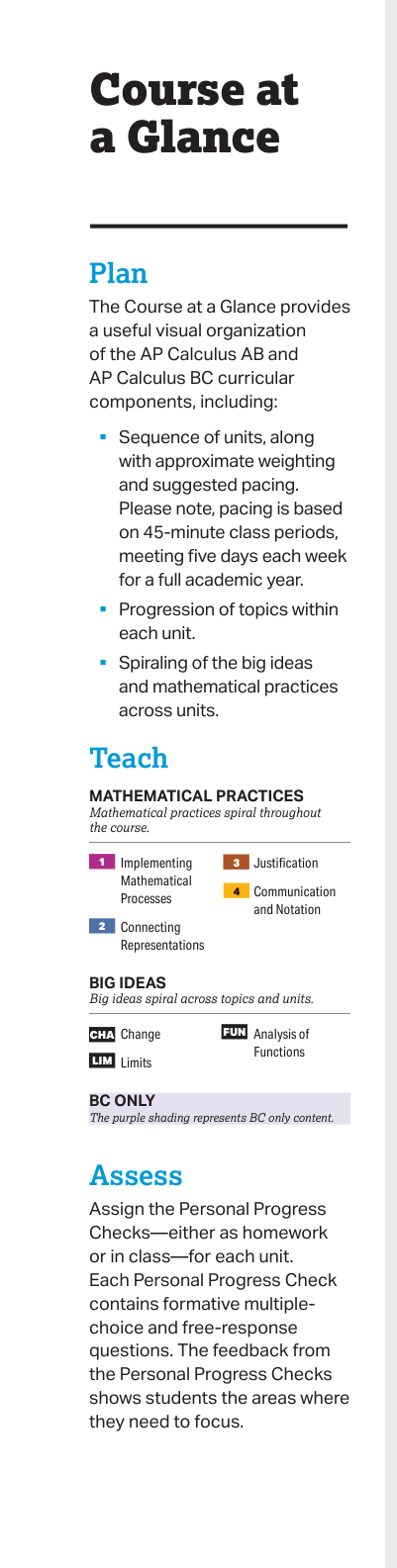
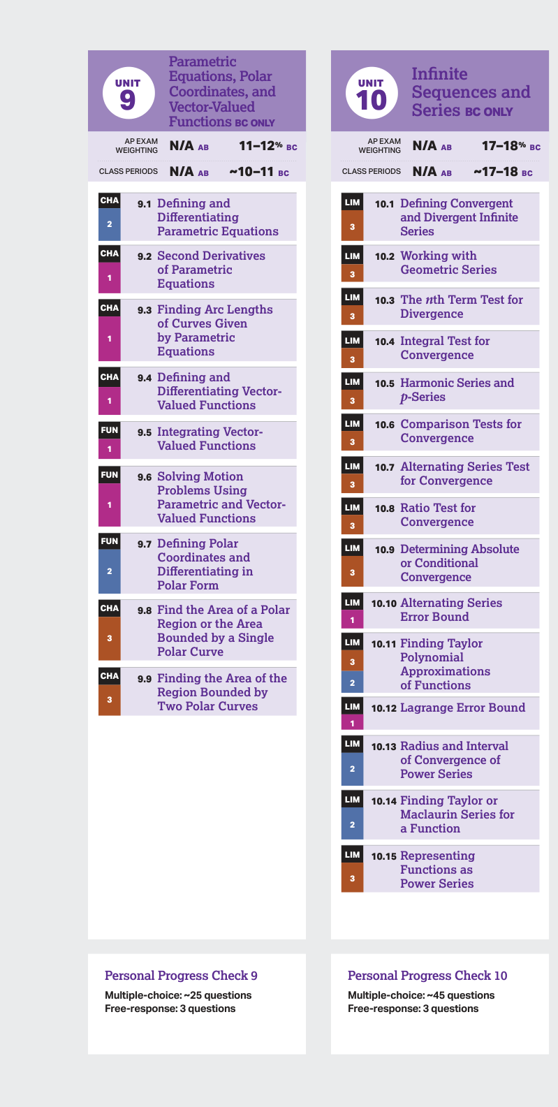
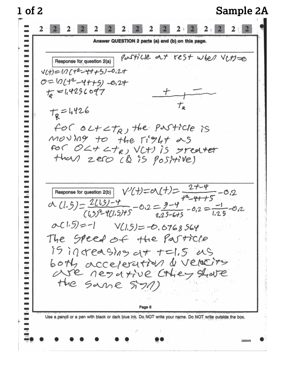
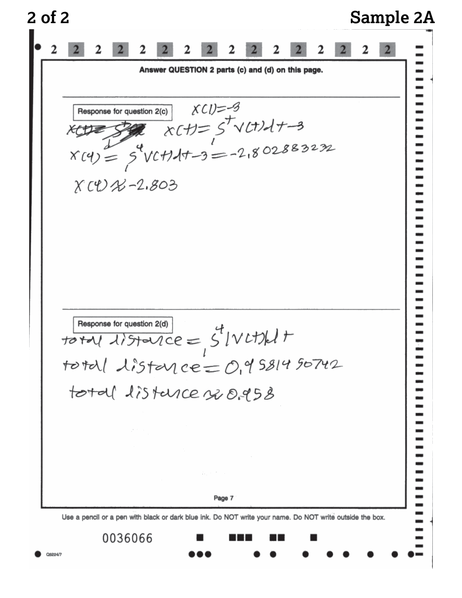
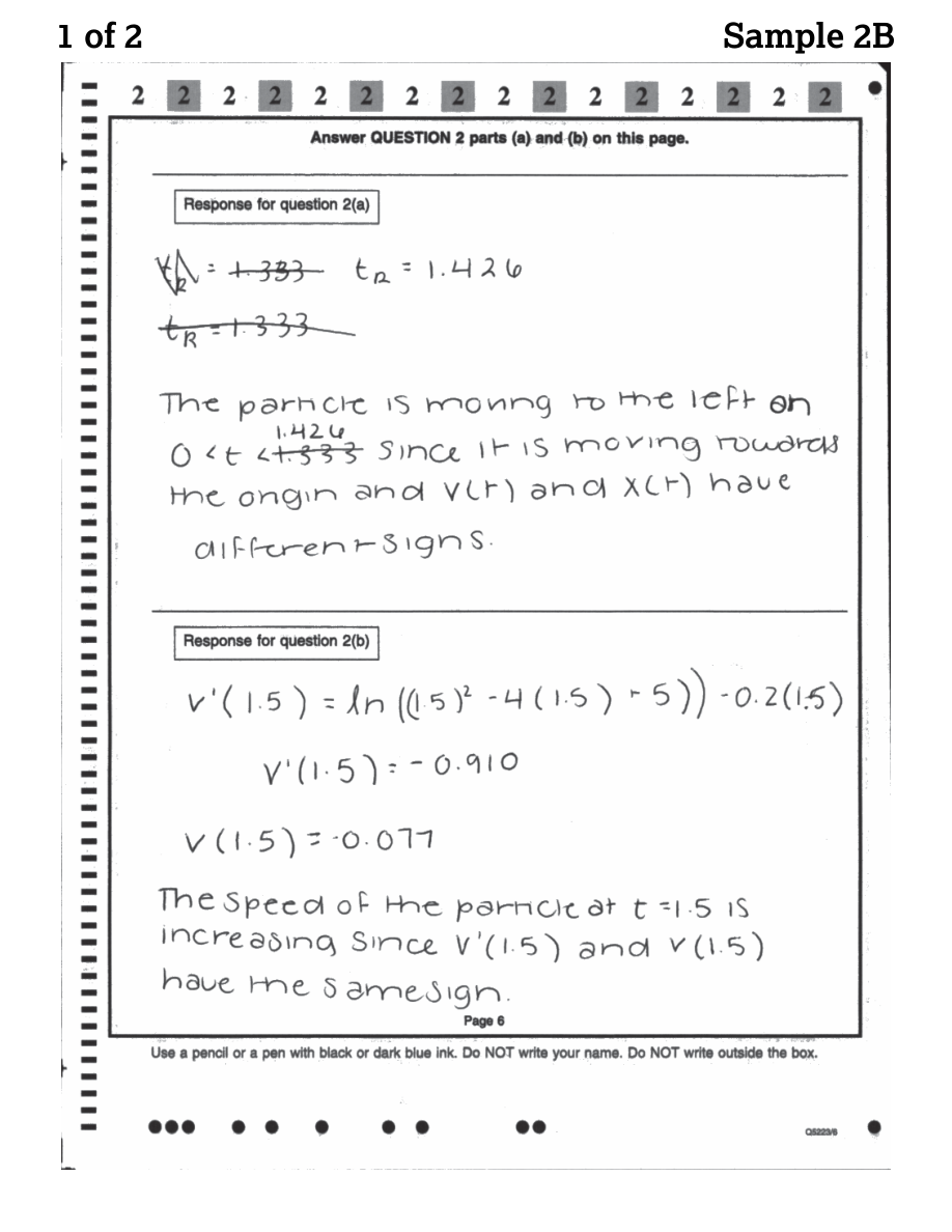
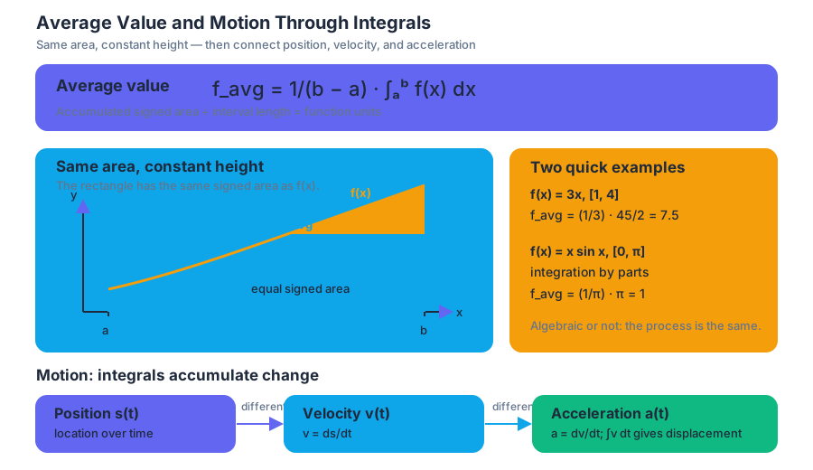
8.2 Connecting Position, Velocity, and Acceleration of Functions Using Integrals
Key concepts: Using definite integrals to connect position, velocity, and acceleration · The Fundamental Theorem of Calculus · Approximated values versus actual values · Numerical methods for approximating definite integrals · Using integrals to solve applied optimization problems
How definite integrals of velocity and acceleration give displacement, final position, change in velocity and total distance traveled for a moving object.
8.2 Connecting Position, Velocity, and Acceleration of Functions Using Integrals
Velocity is the rate of change of position, and acceleration is the rate of change of velocity. Differentiation moves down that chain; a definite integral moves back up it, turning a known rate into the net change it produces over a time interval. This page uses that idea to find displacement, final position, change in velocity and total distance traveled.
Motion: integrals accumulate change
If $v(t)$ is velocity, then integrating velocity gives displacement, the net change in position:
$$ s(b)-s(a)=\int_a^b v(t),dt. $$
If $a(t)$ is acceleration, then integrating acceleration gives the change in velocity:
$$ v(b)-v(a)=\int_a^b a(t),dt. $$
These are applications of the Fundamental Theorem of Calculus: if an accumulation function is defined by an integral, its derivative recovers the rate being accumulated.
Suppose a cyclist has velocity
$$ v(t)=4-t $$
for $0\le t\le5$, measured in meters per second, and starts at position $s(0)=10$ meters. The displacement is
$$ \int_0^5(4-t),dt =\left[4t-\frac{t^2}{2}\right]_0^5 =20-\frac{25}{2} =7.5\text{ meters}. $$
Therefore,
$$ s(5)=10+7.5=17.5\text{ meters}. $$
The cyclist’s total distance traveled is not necessarily $7.5$ meters. Since $v(t)=0$ at $t=4$, the cyclist reverses direction. Total distance is
$$ \int_0^5 |v(t)|,dt =\int_0^4(4-t),dt+\int_4^5(t-4),dt =8+\frac12 =8.5\text{ meters}. $$
Displacement is signed; distance is never negative. Speed is $|v(t)|$, while acceleration is $v'(t)$.
Approximations, numerical integrals, and optimization
When an antiderivative is unavailable or data are given in a table, a definite integral can be approximated with a numerical method such as a left Riemann sum, right Riemann sum, midpoint sum, or trapezoidal sum. An approximation is an estimate of the actual accumulated quantity; its accuracy depends on the method, subinterval widths, and the behavior of the function.
A definite integral can also become an objective function in an applied optimization problem. Suppose a pump’s production rate is
$$ r(t)=12-t^2 $$
units per hour for $0\le t\le T$, and operating the pump incurs a fixed loss of $20$ units. The net accumulated output is
$$ N(T)=\int_0^T(12-t^2),dt-20 =12T-\frac{T^3}{3}-20. $$
To maximize output, differentiate:
$$ N'(T)=12-T^2. $$
The critical point in the feasible interval $0\le T\le5$ is $T=\sqrt{12}\approx3.464$. Checking candidates,
$$ N(0)=-20,\qquad N(5)=60-\frac{125}{3}-20\approx-1.667, $$
and
$$ N(\sqrt{12}) =12\sqrt{12}-\frac{(\sqrt{12})^3}{3}-20 \approx7.713. $$
Thus the maximum net output occurs at approximately $T=3.464$ hours, producing about $7.713$ units. The integral creates the accumulated objective; calculus compares its critical points and endpoints.
Skill 1.E, Finding the average value of a function on an interval, requires correct setup, evaluation or approximation, units, and interpretation. Skill 1.D, Connecting position, velocity, and acceleration of functions using integrals, requires identifying the rate being accumulated and distinguishing net change from total amount. For contextual responses, use the language of EK CHA-4.D.2: the definite integral of a rate of change over an interval gives the net change of the quantity.
Retrieval check: A continuous flow rate is $q(t)$ liters per minute on $[2,8]$. Write, but do not evaluate, the average flow rate and the total volume added. Then state which integral would determine displacement if $q$ were instead velocity.
8.3 Using Accumulation Functions and Definite Integrals in Applied Contexts
Key concepts: Accumulation functions · Definite integrals in applied contexts · Accumulation of change over an interval
How an accumulation function and a definite integral of a rate give the net change of a quantity in context, with correct units and sign.
8.3 Using Accumulation Functions and Definite Integrals in Applied Contexts
A quantity can accumulate even when its rate is changing every moment: water enters a tank at a time-dependent rate, pollutants spread across a region, or energy is used at a varying rate. A definite integral turns that changing rate into the total signed change over an interval.
Accumulation functions: turning a rate into a total
An accumulation function records how much of a quantity has built up from a starting point $a$ to a variable endpoint $x$:
$$ A(x)=\int_a^x r(t),dt, $$
where $r(t)$ is the rate of change of the quantity and $t$ is the input variable. The variable $x$ is the endpoint of accumulation, while $a$ remains fixed.
CHA-4: Definite integrals allow us to solve problems involving the accumulation of change over an interval.
The learning objectives are CHA-4.D: Interpret the meaning of a definite integral in accumulation problems and CHA-4.E: Determine net change using definite integrals in applied contexts. The essential knowledge is expressed through CHA-4.D.1 and CHA-4.E.1: an integral of a rate over an interval represents the accumulated, or net, change in the related quantity.
Suppose $R(t)$ measures water entering a reservoir in liters per minute. Then
$$ \int_2^7 R(t),dt $$
represents the net amount of water entering from minute $t=2$ through minute $t=7$, measured in liters. The units arise automatically:
$$ \left(\frac{\text{liters}}{\text{minute}}\right)(\text{minutes}) =\text{liters}. $$
If $R(t)$ is positive, the reservoir gains water; if $R(t)$ is negative, the model represents net outflow. The integral preserves this sign, so it measures net change, not necessarily total activity.
Worked context: accumulated change
A chemical concentration changes at the rate
$$ C'(t)=4-t $$
milligrams per hour for $0\le t\le 5$. The net change from $t=1$ to $t=5$ is
$$ \int_1^5 (4-t),dt
\left[4t-\frac{t^2}{2}\right]_1^5. $$
Evaluating,
$$ \left(20-\frac{25}{2}\right)
\left(4-\frac12\right)
7.5-3.5
$$
Therefore, the concentration increases by $4$ milligrams over the interval. Notice that the rate becomes negative after $t=4$; the final answer is still positive because the earlier increase is larger than the later decrease.
In applied problems the integral gives only the change, so a final amount also needs the starting amount: $Q(b)=Q(a)+\int_a^b r(t),dt$. If the reservoir holds $500$ liters at $t=2$, it holds $500+\int_2^7 R(t),dt$ liters at $t=7$. When a quantity has both an inflow rate and an outflow rate, integrate their difference. By the Fundamental Theorem of Calculus the accumulation function satisfies $A'(x)=r(x)$, so the sign of the rate tells you where the accumulated amount is increasing or decreasing.
Retrieval check: Oil leaks from a tank at $L(t)$ gallons per hour, and the tank holds $300$ gallons at $t=0$. Write, but do not evaluate, the amount in the tank at $t=6$, and state the units of $\int_0^6 L(t),dt$. The amount is $300-\int_0^6 L(t),dt$, and the integral is measured in gallons.
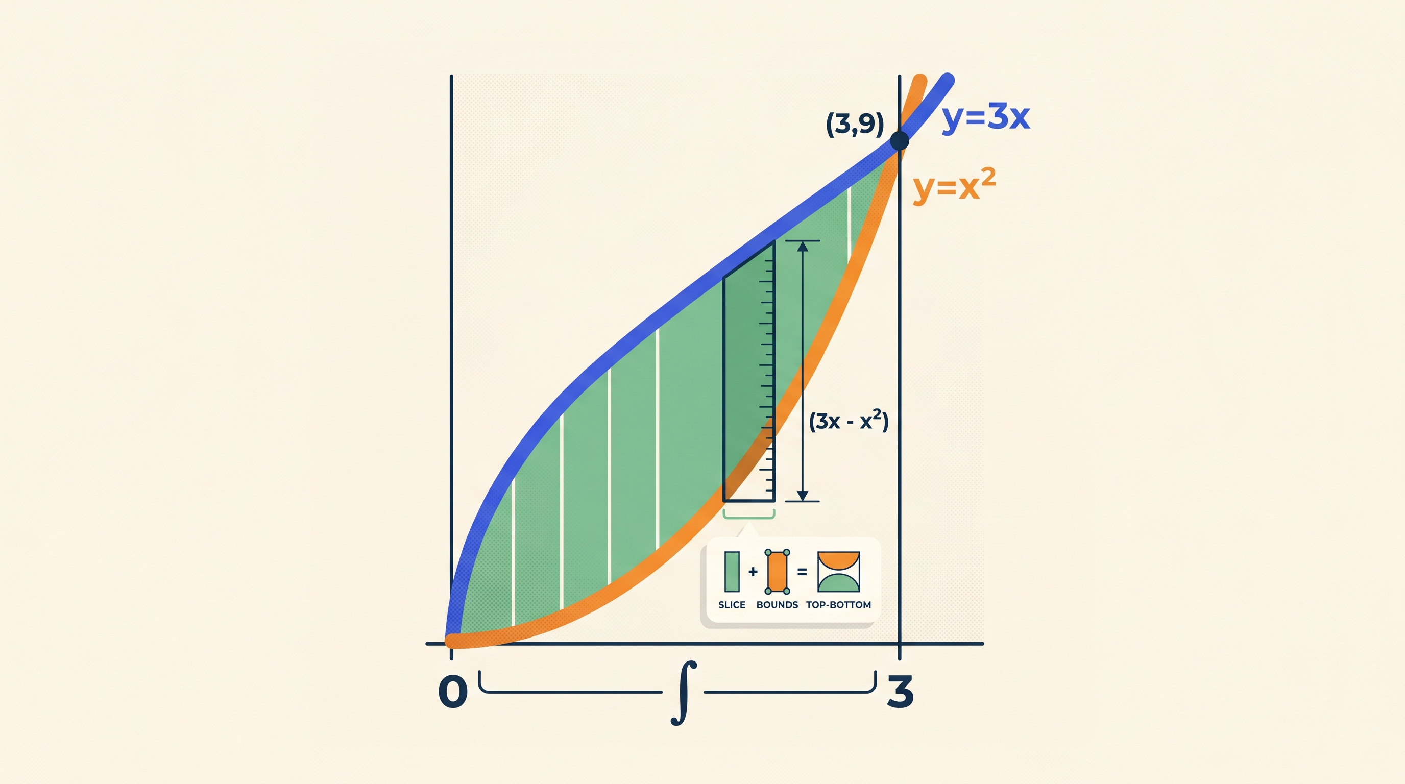
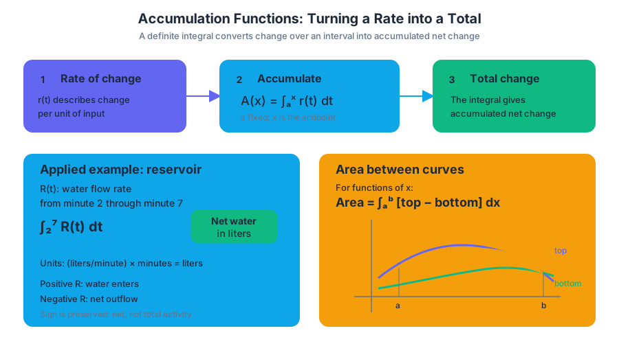
8.4 Finding the Area Between Curves Expressed as Functions of \(x\)
Key concepts: Using definite integrals to find area · Finding the area between curves · Regions bounded by curves expressed as functions of x · Regions bounded by curves expressed as functions of y · Choosing an appropriate mathematical representation for area · Using appropriate mathematical symbols and notation · Interpreting definite integrals geometrically
How to find the area between two curves written as functions of x: find the intersections, decide which curve is on top, and integrate top minus bottom.
8.4 Finding the Area Between Curves Expressed as Functions of (x)
Topic 8.3 used a definite integral to add up a changing rate. The same adding-up works in geometry: cut a region of the plane into thin vertical strips, and the integral of the strip heights is the region's area. This page starts with the area under a single curve, then finds the area enclosed between two curves written as functions of $x$.
Definite integrals as geometric area
When $f(x)\ge 0$ on $[a,b]$, the definite integral
$$ \int_a^b f(x),dx $$
equals the geometric area between the graph of $f$, the $x$-axis, and the vertical lines $x=a$ and $x=b$. If $f(x)$ is below the $x$-axis, the integral is negative because it represents signed area.
CHA-5: Definite integrals allow us to solve problems involving the accumulation of change in area or volume over an interval.
For Topic 8.4, the learning objective is CHA-5.A: Calculate areas in the plane using the definite integral, supported by CHA-5.A.1: Areas of regions in the plane can be calculated with definite integrals. The associated communication skill is 4.C: Use appropriate mathematical symbols and notation. A correct answer requires more than a final decimal: the bounds, integrand, subtraction order, and differential must communicate the region precisely.
Area between curves expressed as functions of $x$
For two curves written as $y=f(x)$ and $y=g(x)$, a vertical slice has height
$$ \text{top}-\text{bottom}. $$
Thus, if $f(x)$ is above $g(x)$ on $[a,b]$,
$$ \boxed{ \text{Area}=\int_a^b\bigl(f(x)-g(x)\bigr),dx }. $$
The bounds $a$ and $b$ usually come from the intersection points, found by solving
$$ f(x)=g(x). $$
Worked example: a region bounded by two curves
Let
$$ f(x)=x+2 \qquad\text{and}\qquad g(x)=x^2. $$
The intersection points satisfy
$$ x+2=x^2, $$
so
$$ x^2-x-2=(x-2)(x+1)=0. $$
Therefore, the region extends from $x=-1$ to $x=2$. On $x=0$, $f(0)=2$ and $g(0)=0$, so $f$ is above $g$. The area is
$$ \int_{-1}^{2}\left[(x+2)-x^2\right]dx. $$
Compute:
$$ \begin{aligned} \text{Area} &=\left[\frac{x^2}{2}+2x-\frac{x^3}{3}\right]_{-1}^{2}\ &=\frac{10}{3}-\left(-\frac{7}{6}\right)\ &=\frac{9}{2}. \end{aligned} $$
The region has area $\frac{9}{2}$ square units.
Choosing the direction of the slices
Integrating with respect to $x$ uses vertical slices, so compare which curve is above the other. Integrating with respect to $y$ uses horizontal slices, so compare which curve is to the right:
$$ \text{horizontal width}=\text{right}-\text{left}. $$
For curves expressed as functions of $y$, the corresponding setup is
$$ \int_c^d\bigl(x_{\text{right}}(y)-x_{\text{left}}(y)\bigr),dy. $$
This is the same geometric idea—adding thin slices—but the next topic develops that $y$-based method in detail.
Misconception check — “Subtracting the curves automatically gives area.” Not always. If the curves cross inside the interval, $f(x)-g(x)$ changes sign and the integral may cancel positive and negative pieces. Find all intersections first, test the ordering on each subinterval, and split the integral whenever the top curve changes.
Retrieval check
A region is bounded by $y=3x$, $y=x^2$, and the $y$-axis. The curves intersect when $3x=x^2$, giving $x=0$ and $x=3$. Since $3x$ is above $x^2$ on $0<x<3$, write the area integral—not its evaluation:
$$ \boxed{\int_0^3(3x-x^2),dx}. $$
The essential questions are always: What does a slice measure? Where are the bounds? Which curve is on top—or, for horizontal slices, which is on the right?
8.5 Finding the Area Between Curves Expressed as Functions of \(y\)
Key concepts: Finding the area between curves expressed as functions of y · Applications of integration · Analytical applications
How to find the area between curves written as x in terms of y, using horizontal slices and integrating right boundary minus left boundary with respect to y.
8.5 Finding the Area Between Curves Expressed as Functions of (y)
When curves are written as $x$-values depending on $y$, the natural “thin slice” is horizontal: its length is right boundary minus left boundary, and its thickness is $dy$. The central question is therefore:
Which curve is farther right at each level $y$, and where do the boundaries exchange positions?
These topics belong to Unit 8, Applications of Integration, under enduring understanding CHA-5. Topic 8.5 Finding the Area Between Curves Expressed as Functions of $y$ emphasizes 1.E: Apply appropriate mathematical rules or procedures, with and without technology. Topic 8.6 Finding the Area Between Curves That Intersect at More Than Two Points emphasizes 2.B: Identify mathematical information from graphical, numerical, analytical, and/or verbal representations.
Horizontal slices: area as right minus left
Suppose two boundaries are given by
$$ x=R(y) \qquad\text{and}\qquad x=L(y). $$
At height $y$, a horizontal slice extends from $x=L(y)$ to $x=R(y)$. Its length is
$$ R(y)-L(y), $$
so the area between the curves from $y=a$ to $y=b$ is
$$ A=\int_a^b\bigl(R(y)-L(y)\bigr),dy, $$
provided the same curve remains rightmost throughout the interval.
The variable of integration determines the geometry. Integrating with respect to $y$ means measuring horizontal distances; integrating with respect to $x$ measures vertical distances. The phrase right minus left is not a new formula to memorize—it is a description of the length of each horizontal slice.
Worked example: one $dy$ integral
Find the area enclosed by $x=y^2$ and $x=y+2$. Setting $y^2=y+2$ gives $(y-2)(y+1)=0$, so the curves meet at $y=-1$ and $y=2$. At the test level $y=0$ the line is at $x=2$ and the parabola is at $x=0$, so the line is the right boundary and $A=\int_{-1}^{2}\bigl[(y+2)-y^2\bigr],dy$. An antiderivative is $\frac{y^2}{2}+2y-\frac{y^3}{3}$, which gives $A=\frac{10}{3}-\left(-\frac{7}{6}\right)=\frac{9}{2}$ square units. Vertical slices would need two integrals here, because for $0\le x\le 1$ the parabola $x=y^2$ is both the top and the bottom of the region.
Retrieval check
Suppose $x=y^2-1$ and $x=y+1$ intersect at $y=-1$ and $y=2$. At $y=0$, the values are $-1$ and $1$, so $x=y+1$ is the right boundary. At $y=1$, the values are $0$ and $2$, so it is still right. The area is therefore set up as
$$ \int_{-1}^{2}\left[(y+1)-(y^2-1)\right],dy. $$
If a graph or table showed an additional intersection inside $[-1,2]$, the correct response would be to split the integral there and recheck which curve is right on each resulting interval. That decision—not the antiderivative—is the essential reasoning in these problems.
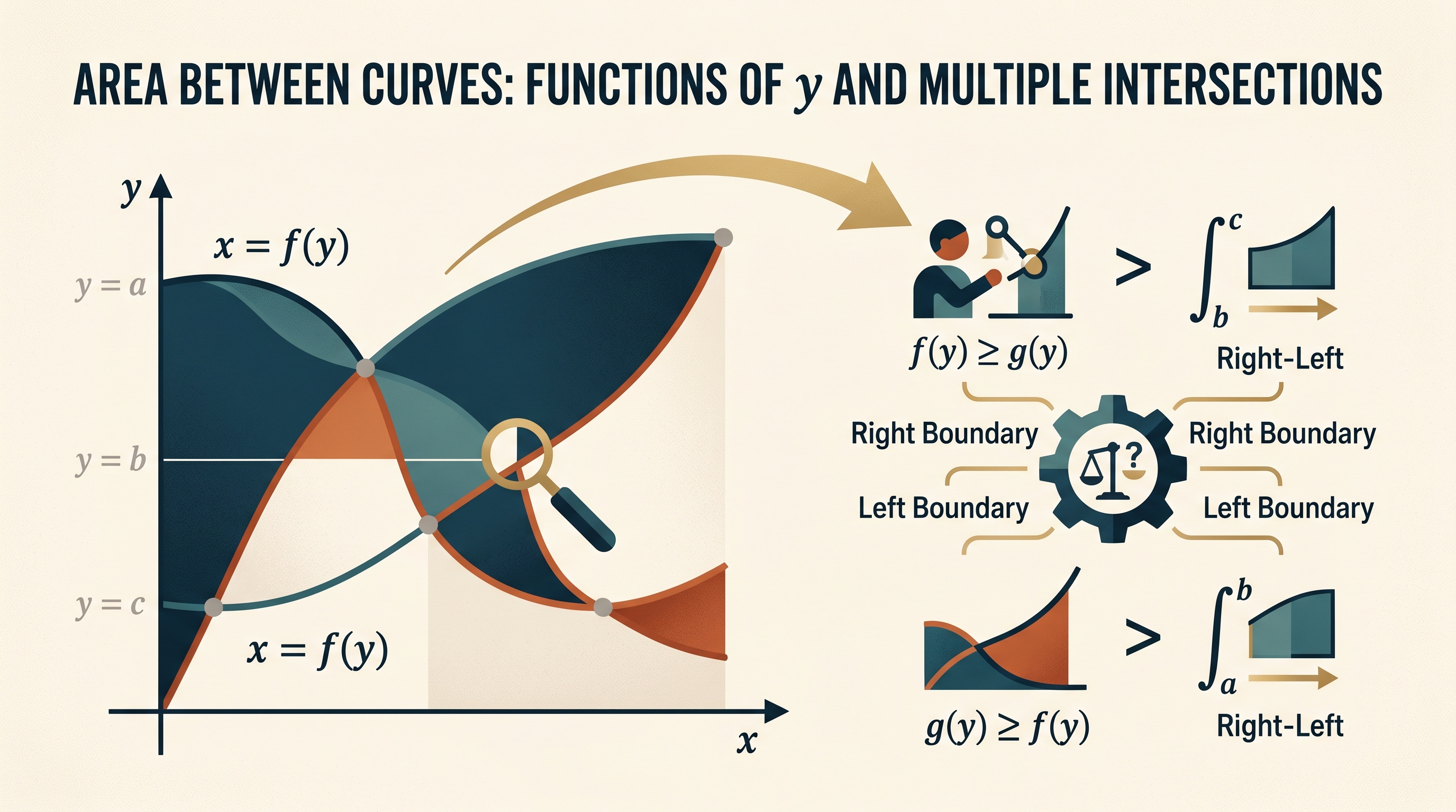
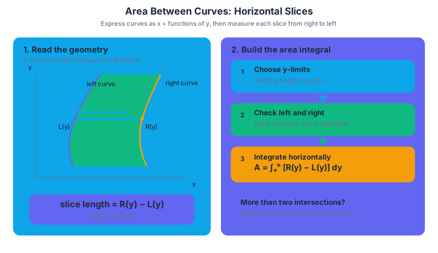
8.6 Finding the Area Between Curves That Intersect at More Than Two Points
Key concepts: Finding the area between curves that intersect at more than two points · Applications of integration · Analytical applications · Identifying mathematical information from graphical and numerical representations
How to find the area between curves that cross more than twice by splitting the integral at every intersection and rechecking which curve is ahead on each piece.
8.6 Finding the Area Between Curves That Intersect at More Than Two Points
Two curves can cross more than twice, and at each crossing they may trade places, so one integral over the whole span mixes positive and negative pieces and no longer measures area. Topic 8.6 Finding the Area Between Curves That Intersect at More Than Two Points sits under enduring understanding CHA-5 and emphasizes 2.B: Identify mathematical information from graphical, numerical, analytical, and/or verbal representations. The main example uses curves written as $x$ in terms of $y$, where each horizontal slice has length right minus left (Topic 8.5).
Worked example: intersections at more than two $y$-levels
Consider the curves
$$ x=\sin y \qquad\text{and}\qquad x=0 $$
for $0\le y\le 2\pi$. A graph or numerical table reveals three intersection levels:
$$ \sin y=0 \quad\Longrightarrow\quad y=0,\ \pi,\ 2\pi. $$
The key information is not merely where the curves meet, but which curve lies to the right between consecutive intersections.
| $y$ | $\sin y$ | $x=0$ | Right boundary | Left boundary |
|---|---|---|---|---|
| $0$ | $0$ | $0$ | tie | tie |
| $\frac{\pi}{2}$ | $1$ | $0$ | $x=\sin y$ | $x=0$ |
| $\pi$ | $0$ | $0$ | tie | tie |
| $\frac{3\pi}{2}$ | $-1$ | $0$ | $x=0$ | $x=\sin y$ |
| $2\pi$ | $0$ | $0$ | tie | tie |
On $0<y<\pi$, $\sin y>0$, so $x=\sin y$ is right of $x=0$. On $\pi<y<2\pi$, $\sin y<0$, so $x=\sin y$ is left of $x=0$. Because the boundaries switch positions at $y=\pi$, one integral with a fixed subtraction would produce a negative contribution on the second interval.
The area must therefore be written piecewise:
$$ \begin{aligned} A &=\int_0^\pi\bigl(\sin y-0\bigr),dy +\int_\pi^{2\pi}\bigl(0-\sin y\bigr),dy\[4pt] &=\left[-\cos y\right]0^\pi +\left[\cos y\right]\pi^{2\pi}\[4pt] &=2+2\ &=4. \end{aligned} $$
The result is $4$ square units. The sign change in $\sin y$ does not mean the geometric area is negative; it means the identity of the right and left curves changes.
The same rule with vertical slices
Curves written as functions of $x$ are handled the same way, with top minus bottom. The curves $y=x^3$ and $y=x$ meet at $x=-1$, $0$ and $1$. The cubic is on top on $(-1,0)$ and the line is on top on $(0,1)$, so $A=\int_{-1}^{0}(x^3-x),dx+\int_{0}^{1}(x-x^3),dx=\frac14+\frac14=\frac12$. The single integral $\int_{-1}^{1}(x^3-x),dx$ equals $0$, which is clearly not the area.
How representations work together
A graphical representation helps locate intersection levels and shows which curve is horizontally farther right. A numerical representation confirms the sign of the horizontal difference at test values. An analytical representation supplies the equation used to solve for intersections, while a verbal representation communicates the setup clearly: “Integrate right boundary minus left boundary on each interval.”
For two functions $x=f(y)$ and $x=g(y)$, define their horizontal difference by
$$ D(y)=f(y)-g(y). $$
Then:
- if $D(y)>0$, $f$ is right of $g$;
- if $D(y)<0$, $g$ is right of $f$;
- if $D(y)=0$, the curves intersect.
This is the work of 2.B: Identify mathematical information from graphical, numerical, analytical, and/or verbal representations. The representation tells you where to split the integral; the procedure in 1.E then evaluates the resulting expression, with or without technology.
Misconception check: “The bounds are enough”
Misconception — using only the outer bounds. If curves intersect more than twice, the entire region may not have one consistent right-minus-left expression. Integrating from the lowest to highest $y$-value without splitting at every relevant intersection can subtract the boundaries in the wrong order and yield a signed result rather than total area.
Misconception — taking $\int(f-g),dy$ and trusting the answer. A definite integral measures signed accumulation. Geometric area requires nonnegative slice lengths, so either reverse the subtraction on intervals where the curves switch or integrate $\lvert f(y)-g(y)\rvert$ after identifying all intersections.
8.7 Volumes with Cross Sections: Squares and Rectangles
Key concepts: Volumes with cross sections · Squares and rectangular cross sections · Definite integrals as accumulation · Using a given region as the base of a solid · Area formulas for geometric cross sections · Setting up volume integrals · Calculating total volume · Distinguishing among volume problem types
How to find the volume of a solid whose cross sections are squares or rectangles by writing the slice area from the base region and integrating it.
8.7 Volumes with Cross Sections: Squares and Rectangles
A solid can have a different shape at every horizontal or vertical position, yet its total volume is still an accumulation: add the areas of infinitely many thin slices. If the cross-sectional area at position $x$ is $A(x)$, then
$$ V=\int_a^b A(x),dx. $$
Here, $A(x)$ is not guessed from the three-dimensional picture. It is built from the geometric shape assigned to each slice.
The central translation: from a base region to a solid
A problem begins with a base region, usually bounded by curves. At each $x$-value, a slice through that region has a measurable length. The problem then specifies what two-dimensional shape is erected on that slice: a square, rectangle, triangle, semicircle, or another geometric figure.
The essential workflow is:
- Identify the interval $[a,b]$.
- Find the slice dimensions from the boundary curves.
- Use the specified cross-sectional shape to write $A(x)$.
- Accumulate those areas with $\int_a^b A(x),dx$.
This is different from a problem that merely asks for the area of a planar region. The base region supplies the dimensions of the slices; the specified cross sections determine the three-dimensional volume. Do not replace the stated shape with a rotation formula: use the cross-sectional geometry the problem gives.
Squares and rectangles
For a square whose side length is $s(x)$,
$$ A(x)=[s(x)]^2. $$
For a rectangle with length $l(x)$ and width $w(x)$,
$$ A(x)=l(x)w(x). $$
The required course knowledge is captured by CHA-5.B.1: volumes of solids with square and rectangular cross sections are found by combining definite integrals with the corresponding area formulas.
Worked example: rectangular cross sections
Let the base be the region between $y=x^2$ and $y=2x$ from $x=0$ to $x=2$. At each $x$, the vertical slice has width
$$ w(x)=2x-x^2. $$
Suppose each cross section perpendicular to the $x$-axis is a rectangle whose length is twice its width. Then
$$ l(x)=2w(x)=2(2x-x^2), $$
so its area is
$$ A(x)=l(x)w(x) =2(2x-x^2)^2. $$
Therefore, the volume is
$$ V=\int_0^2 2(2x-x^2)^2,dx =\frac{32}{15}. $$
The important step is not the final antiderivative. It is translating the graph into the slice dimension $2x-x^2$, then translating the rectangle description into $A(x)$.
Square cross sections on the same base. If each cross section perpendicular to the $x$-axis is instead a square whose side is the slice width $w(x)=2x-x^2$, then $A(x)=(2x-x^2)^2$ and $V=\int_0^2(2x-x^2)^2,dx=\int_0^2\left(4x^2-4x^3+x^4\right)dx=\frac{32}{3}-16+\frac{32}{5}=\frac{16}{15}$. Only the area formula changed; the base region, the bounds and the slice length are the same.
Skill focus: justification
The suggested AP skill is 3.D — Apply an appropriate mathematical definition, theorem, or test. In these problems, justification means making the geometry visible in the equation: state the slice dimension, identify whether it is a side, length, base, height, or diameter, and then apply the correct area formula.
Misconception check — “The base region is already the volume.” A planar region has area, not volume. The region only provides the dimensions of infinitely many cross sections. Volume appears after those cross-sectional areas are accumulated with a definite integral.
Retrieval check: A vertical slice of a base region has length $d(x)$. What is the integrand if each cross section is a square with side $d(x)$? What if each is a rectangle with base $d(x)$ and constant height $3$? The answers are $[d(x)]^2$ and $3d(x)$: only a dimension taken from the slice varies with $x$, and a square uses it twice.
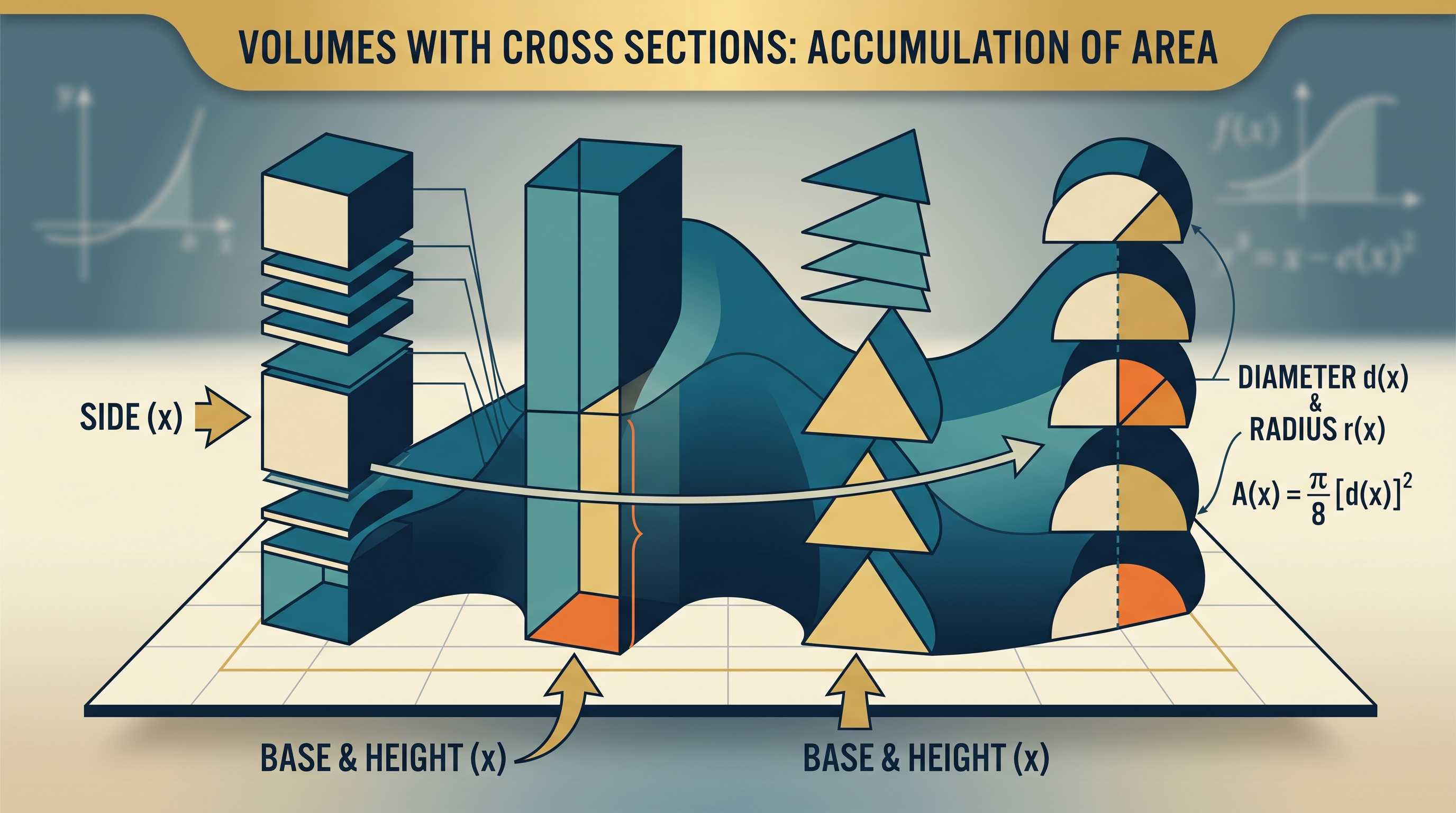

8.8 Volumes with Cross Sections: Triangles and Semicircles
Key concepts: Volumes with cross sections · Triangles and semicircular cross sections · Definite integrals as accumulation · Using a given region as the base of a solid · Area formulas for geometric cross sections · Setting up volume integrals · Translating graphs of intersecting curves into integrals · Calculating total volume · Distinguishing among volume problem types
How to find the volume of a solid whose cross sections are triangles or semicircles, including the one-half and pi-over-eight factors in the slice area.
8.8 Volumes with Cross Sections: Triangles and Semicircles
Topic 8.7 built solids from square and rectangular slices and found their volumes with $V=\int_a^b A(x),dx$, where $A(x)$ is the area of the cross section at $x$. The same accumulation works for any slice shape whose area you can write down. This page uses triangles and semicircles, where the area formula brings in a factor of $\frac12$ or $\frac{\pi}{8}$ that is easy to lose.
A problem begins with a base region, usually bounded by curves. At each $x$-value, a slice through that region has a measurable length. The problem then specifies what two-dimensional shape is erected on that slice: a square, rectangle, triangle, semicircle, or another geometric figure.
The essential workflow is:
- Identify the interval $[a,b]$.
- Find the slice dimensions from the boundary curves.
- Use the specified cross-sectional shape to write $A(x)$.
- Accumulate those areas with $\int_a^b A(x),dx$.
This is different from a problem that merely asks for the area of a planar region. The base region supplies the dimensions of the slices; the specified cross sections determine the three-dimensional volume. Do not replace the stated shape with a rotation formula: use the cross-sectional geometry the problem gives.
Triangular cross sections from intersecting curves
For a triangle,
$$ A=\frac12 bh, $$
where $b$ is the base and $h$ is the perpendicular height. The base region determines one or both of these dimensions; the wording must tell you how the triangle is constructed.
Worked example: triangular cross sections
Consider the region bounded by $y=x$ and $y=x^2$ for $0\le x\le1$. Since $x\ge x^2$ on this interval, the vertical slice length is
$$ d(x)=x-x^2. $$
Suppose each cross section perpendicular to the $x$-axis is a right triangle whose base and height both equal this slice length. Thus,
$$ b(x)=d(x)=x-x^2, \qquad h(x)=d(x)=x-x^2. $$
The cross-sectional area becomes
$$ A(x)=\frac12(x-x^2)(x-x^2) =\frac12(x-x^2)^2. $$
The volume is therefore
$$ V=\int_0^1 \frac12(x-x^2)^2,dx =\frac1{60}. $$
Notice how the bounds $0$ and $1$ come from the intersections of the curves: solving $x=x^2$ gives $x=0$ and $x=1$. The graph supplies both the limits and the slice length.
Two other triangles are common on the exam. An equilateral triangle with side $d(x)$ has area $\frac{\sqrt3}{4}[d(x)]^2$, and an isosceles right triangle whose hypotenuse is $d(x)$ has area $\frac14[d(x)]^2$.
Semicircular cross sections
If the slice length is the diameter $d(x)$ of a semicircle, then its radius is
$$ r(x)=\frac{d(x)}{2}. $$
Using the semicircle area formula,
$$ A(x)=\frac12\pi r(x)^2 =\frac12\pi\left(\frac{d(x)}2\right)^2 =\frac{\pi}{8}[d(x)]^2. $$
For the same base region between $y=x$ and $y=x^2$ on $[0,1]$, if each cross section is a semicircle with diameter equal to the vertical slice length, then $d(x)=x-x^2$ and
$$ V=\int_0^1 \frac{\pi}{8}(x-x^2)^2,dx =\frac{\pi}{240}. $$
The factor $\frac{\pi}{8}$ matters: using $\pi[d(x)]^2$ would treat the diameter as the radius and produce a volume four times too large.
The suggested AP skill is 3.D — Apply an appropriate mathematical definition, theorem, or test. In these problems, justification means making the geometry visible in the equation: state the slice dimension, identify whether it is a side, length, base, height, or diameter, and then apply the correct area formula.
Misconception check — “The base region is already the volume.” A planar region has area, not volume. The region only provides the dimensions of infinitely many cross sections. Volume appears after those cross-sectional areas are accumulated with a definite integral.
Retrieval check: A vertical slice has length $d(x)$, and each cross section is a semicircle with diameter $d(x)$. What is the integrand? The answer is
$$ A(x)=\frac{\pi}{8}[d(x)]^2, $$
because the radius is half the diameter.
8.9 Volume with Disc Method: Revolving Around the \(x\)- or \(y\)-Axis
Key concepts: Applications of integration · Volumes of solids of revolution · Disc method · Revolving regions around the x-axis · Revolving regions around the y-axis · Using definite integrals to calculate volume · Applying an appropriate mathematical definition, theorem, or test · Topic 8.9: Volume with Disc Method: Revolving Around the x- or y-Axis · Learning objective CHA-5.C
How the disc method gives the volume of a region revolved around the x-axis or the y-axis by integrating pi times the radius squared.
8.9 Volume with Disc Method: Revolving Around the (x)- or (y)-Axis
A flat region becomes a three-dimensional solid when it spins around an axis, and its volume can be found by adding the areas of infinitely many thin circular slices. The disc method turns that idea into a definite integral.
Learning Objective CHA-5.C: Calculate volumes of solids of revolution using definite integrals.
Essential Knowledge CHA-5.C.1: Volumes of solids of revolution around the $x$- or $y$-axis may be found by using definite integrals with the disc method.
The central question is: What is the area of a cross section perpendicular to the axis of rotation? If the cross section is a filled circle, its area is
$$ A=\pi r^2, $$
where $r$ is the distance from the axis of rotation to the boundary of the region. Adding these cross-sectional areas across an interval gives
$$ V=\int A,d(\text{position}). $$
The disc method around the $x$-axis
When a region under a nonnegative function $y=f(x)$ is revolved around the $x$-axis, a vertical slice becomes a circular disc. The radius is the vertical distance from the $x$-axis to the curve, so $r=f(x)$, and the thickness is $dx$:
$$ V=\int_a^b \pi [f(x)]^2,dx. $$
Worked example: rotating around the $x$-axis
Rotate the region bounded by $y=x^2$, the $x$-axis, $x=0$, and $x=2$ around the $x$-axis.
At a particular value of $x$, the slice has radius
$$ r=y=x^2. $$
Therefore its cross-sectional area is
$$ A(x)=\pi(x^2)^2=\pi x^4. $$
The volume is
$$ \begin{aligned} V&=\int_0^2 \pi x^4,dx\ &=\pi\left[\frac{x^5}{5}\right]_0^2\ &=\frac{32\pi}{5}. \end{aligned} $$
Thus the solid has volume
$$ \boxed{\frac{32\pi}{5}\text{ cubic units}}. $$
The square is essential: the function gives a length, namely the radius, while volume requires a cross-sectional area. Squaring $f(x)$ converts the radius into the area factor $\pi[f(x)]^2$.
The disc method around the $y$-axis
For rotation around the $y$-axis, horizontal slices are perpendicular to the axis. If the region is described by $x=g(y)$, then the radius is the horizontal distance from the $y$-axis:
$$ r=g(y). $$
The volume becomes
$$ V=\int_c^d \pi[g(y)]^2,dy. $$
The limits must now be $y$-values, because the slices have thickness $dy$.
Worked example: rotating around the $y$-axis
Consider the region bounded by $x=y^2$, the $y$-axis, $y=0$, and $y=2$, revolved around the $y$-axis. A horizontal slice extends from $x=0$ to $x=y^2$, so its radius is $y^2$.
$$ A(y)=\pi(y^2)^2=\pi y^4. $$
Therefore,
$$ \begin{aligned} V&=\int_0^2 \pi y^4,dy\ &=\pi\left[\frac{y^5}{5}\right]_0^2\ &=\boxed{\frac{32\pi}{5}}. \end{aligned} $$
Although the equations differ in appearance, both examples use the same structure:
$$ \boxed{\text{volume}=\int \text{area of a perpendicular cross section},d(\text{position})}. $$
Before you integrate
Misconception: Every volume integral should use $dx$.
Correction: The variable is determined by the direction of the slices. Rotation around a horizontal axis uses vertical slices and usually $dx$; rotation around a vertical axis uses horizontal slices and usually $dy$.
Before integrating, verify three choices:
- Are the slices perpendicular to the axis?
- Is the radius a distance to that axis?
- Do the limits describe the full range of the slicing variable?
The justification skill 3.D — Justification requires more than writing an integral: the radius, limits, and cross-sectional area must match the geometry.
Retrieval check: The region bounded by $x=\sqrt{y}$, the $y$-axis and the line $y=2$ is revolved around the $y$-axis. Which way do the slices run, and what is the volume? Horizontal slices are perpendicular to the $y$-axis, each with radius $\sqrt{y}$, so $V=\int_0^2\pi(\sqrt{y})^2,dy=\int_0^2\pi y,dy=2\pi$.
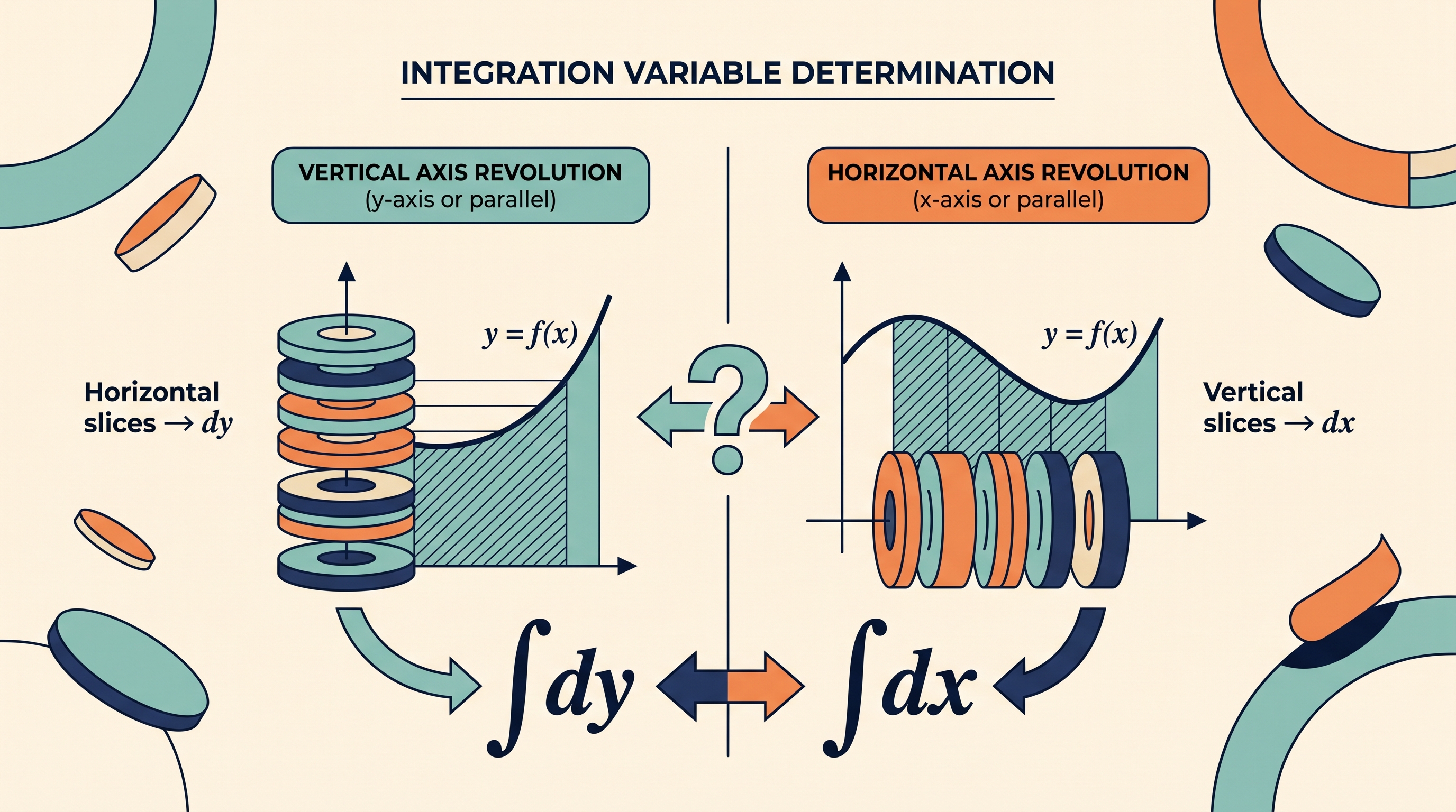
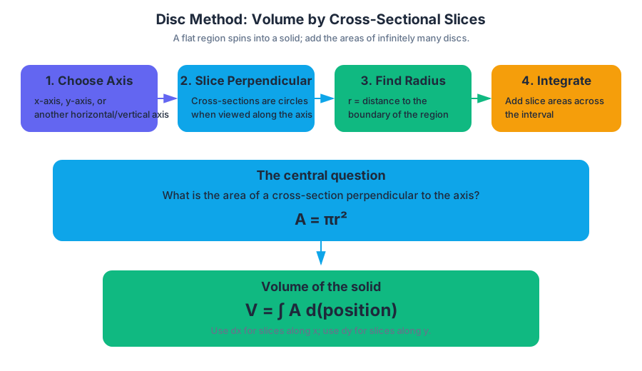
8.10 Volume with Disc Method: Revolving Around Other Axes
Key concepts: Applications of integration · Volumes of solids of revolution · Disc method · Using definite integrals to calculate volume · Applying an appropriate mathematical definition, theorem, or test · Topic 8.10: Volume with Disc Method: Revolving Around Other Axes · Learning objective CHA-5.C
How to use the disc method when a region is revolved around a horizontal or vertical line other than an axis, measuring each radius as a distance to that line.
8.10 Volume with Disc Method: Revolving Around Other Axes
A region does not have to spin around a coordinate axis. A bowl, a bead or a machine part may be modeled by revolving a region around a line such as $y=1$ or $x=-1$. The disc method from Topic 8.9 still applies, as long as each slice is perpendicular to the line and its radius is measured from that line.
The central question is: What is the area of a cross section perpendicular to the axis of rotation? If the cross section is a filled circle, its area is
$$ A=\pi r^2, $$
where $r$ is the distance from the axis of rotation to the boundary of the region. Adding these cross-sectional areas across an interval gives
$$ V=\int A,d(\text{position}). $$
Topic 8.10: revolving around other axes
Topic 8.10 extends the disc-method idea to horizontal or vertical axes that are not the coordinate axes. The radius is always a distance to the axis, not automatically the value of the function.
For a horizontal axis $y=k$,
$$ r=\lvert f(x)-k\rvert. $$
For a vertical axis $x=h$, use horizontal slices and measure
$$ r=\lvert g(y)-h\rvert. $$
The suggested skill 2.D — Connecting Representations is visible here: the graph identifies the radius, the algebra expresses that distance, and the integral accumulates the resulting areas.
Worked example: rotation around $y=1$
Rotate the region between $y=1$ and $y=1+\sqrt{x}$, for $0\le x\le4$, around the line $y=1$. Each vertical slice touches the axis of rotation, so it produces a disc with radius
$$ r=(1+\sqrt{x})-1=\sqrt{x}. $$
Hence,
$$ \begin{aligned} V&=\int_0^4 \pi(\sqrt{x})^2,dx\ &=\int_0^4 \pi x,dx\ &=\pi\left[\frac{x^2}{2}\right]_0^4\ &=\boxed{8\pi\text{ cubic units}}. \end{aligned} $$
A vertical axis can be handled similarly by rewriting the region in terms of $y$. For example, rotate the region
$$ 0\le y\le2,\qquad -1\le x\le y-1 $$
around $x=-1$. A horizontal slice has radius
$$ r=(y-1)-(-1)=y, $$
so
$$ V=\int_0^2 \pi y^2,dy=\frac{8\pi}{3}. $$
Misconception check: “The limits always come from $x$”
Misconception: Every volume integral should use $dx$.
Correction: The variable is determined by the direction of the slices. Rotation around a horizontal axis uses vertical slices and usually $dx$; rotation around a vertical axis uses horizontal slices and usually $dy$.
Before integrating, verify three choices:
- Are the slices perpendicular to the axis?
- Is the radius a distance to that axis?
- Do the limits describe the full range of the slicing variable?
The justification skill 3.D — Justification requires more than writing an integral: the radius, limits, and cross-sectional area must match the geometry.
Retrieval check: A region under $y=f(x)$ from $x=a$ to $x=b$ is rotated around $y=k$. If every vertical slice reaches the axis, what integral represents the volume?
The answer is
$$ \boxed{V=\int_a^b \pi\bigl(f(x)-k\bigr)^2,dx} $$
when $f(x)\ge k$ on the interval. The function supplies the radius only after its distance from the axis has been identified.
8.11 Volume with Washer Method: Revolving Around the \(x\)- or \(y\)-Axis
Key concepts: Washer method for finding volumes of solids of revolution · Disk and washer cross sections as ring-shaped regions · Volumes of revolution around the x-axis or y-axis · Using definite integrals to represent volume · Determining outer and inner radii from distances to the line of revolution · Formula V = π∫(R^2 - r^2) for washer volumes · Connecting a geometric solid to its integral representation · Applying appropriate rounding procedures
How the washer method gives the volume of a region revolved around the x-axis or y-axis by integrating pi times outer radius squared minus inner radius squared.
8.11 Volume with Washer Method: Revolving Around the (x)- or (y)-Axis
A rotating region does not always produce a solid cylinder. When each perpendicular slice leaves a hole in the middle, the slice is a washer: a ring-shaped cross section whose area is the area of the outer disk minus the area of the inner disk.
Washer area:
$$A=\pi\left(R^2-r^2\right)$$
Here, $R$ is the outer radius and $r$ is the inner radius.
The washer method accumulates these cross-sectional areas with a definite integral. If vertical slices are used, the volume is
$$V=\pi\int_a^b\left[R(x)^2-r(x)^2\right],dx.$$
For horizontal slices, the corresponding form is
$$V=\pi\int_c^d\left[R(y)^2-r(y)^2\right],dy.$$
The variable of integration is determined by the direction of the slices, not merely by the appearance of the functions.
Choosing the slice direction
A slice must be perpendicular to the axis of rotation. Rotation about a horizontal line produces washers from vertical slices, so the integral is usually written with respect to $x$. Rotation about a vertical line produces washers from horizontal slices, so the integral is usually written with respect to $y$.
For rotation around the coordinate axes, radii are measured from the appropriate axis:
- Around the $x$-axis, a vertical distance in $y$ becomes a radius.
- Around the $y$-axis, a horizontal distance in $x$ becomes a radius.
- Around a shifted horizontal line $y=k$, radius means vertical distance $\lvert y-k\rvert$.
- Around a shifted vertical line $x=h$, radius means horizontal distance $\lvert x-h\rvert$.
The crucial question is always: Which boundary is farther from the line of revolution?
Worked example: the region between $y=x$ and $y=x^2$
The curves $y=x$ and $y=x^2$ meet at $x=0$ and $x=1$, and the line is on top between them. Revolved around the $x$-axis, a vertical slice sweeps out a washer with outer radius $R(x)=x$ and inner radius $r(x)=x^2$, so $V=\pi\int_0^1\left(x^2-x^4\right)dx=\pi\left(\frac13-\frac15\right)=\frac{2\pi}{15}$.
Revolved around the $y$-axis, the slices must be horizontal, so rewrite the boundaries as $x=y$ and $x=\sqrt{y}$. Now the parabola is farther from the axis: $R(y)=\sqrt{y}$ and $r(y)=y$, so $V=\pi\int_0^1\left(y-y^2\right)dy=\pi\left(\frac12-\frac13\right)=\frac{\pi}{6}$. The radii are squared separately; $\pi(R-r)^2$ is not the area of a washer.
Washer method or cylindrical shells?
Use washers when slices are perpendicular to the axis and rotation creates an outer radius with a possible inner radius. Use cylindrical shells when slices are parallel to the axis and the natural factors are circumference times height:
$$dV=2\pi(\text{radius})(\text{height}),dx.$$
A disk is simply the special case $r=0$; a washer has $r>0$.
The AP skill 2.D — Connecting Representations appears when you connect the rectangle, its rotated washer, the radius functions, and the definite integral. The AP skill 4.E — Use appropriate mathematical symbols, notation, and language matters when you identify $R$, $r$, bounds, units, and a properly rounded numerical result.
Misconception check: The “outer” radius is not necessarily the larger function value. It is the larger distance to the rotation line.
Retrieval check: The region between $y=\sqrt{x}$ and $y=2$ for $0\le x\le 4$ is revolved around the $x$-axis. Identify $R(x)$ and $r(x)$ and write the integral. Here $R(x)=2$ and $r(x)=\sqrt{x}$, so $V=\pi\int_0^4(4-x),dx$.
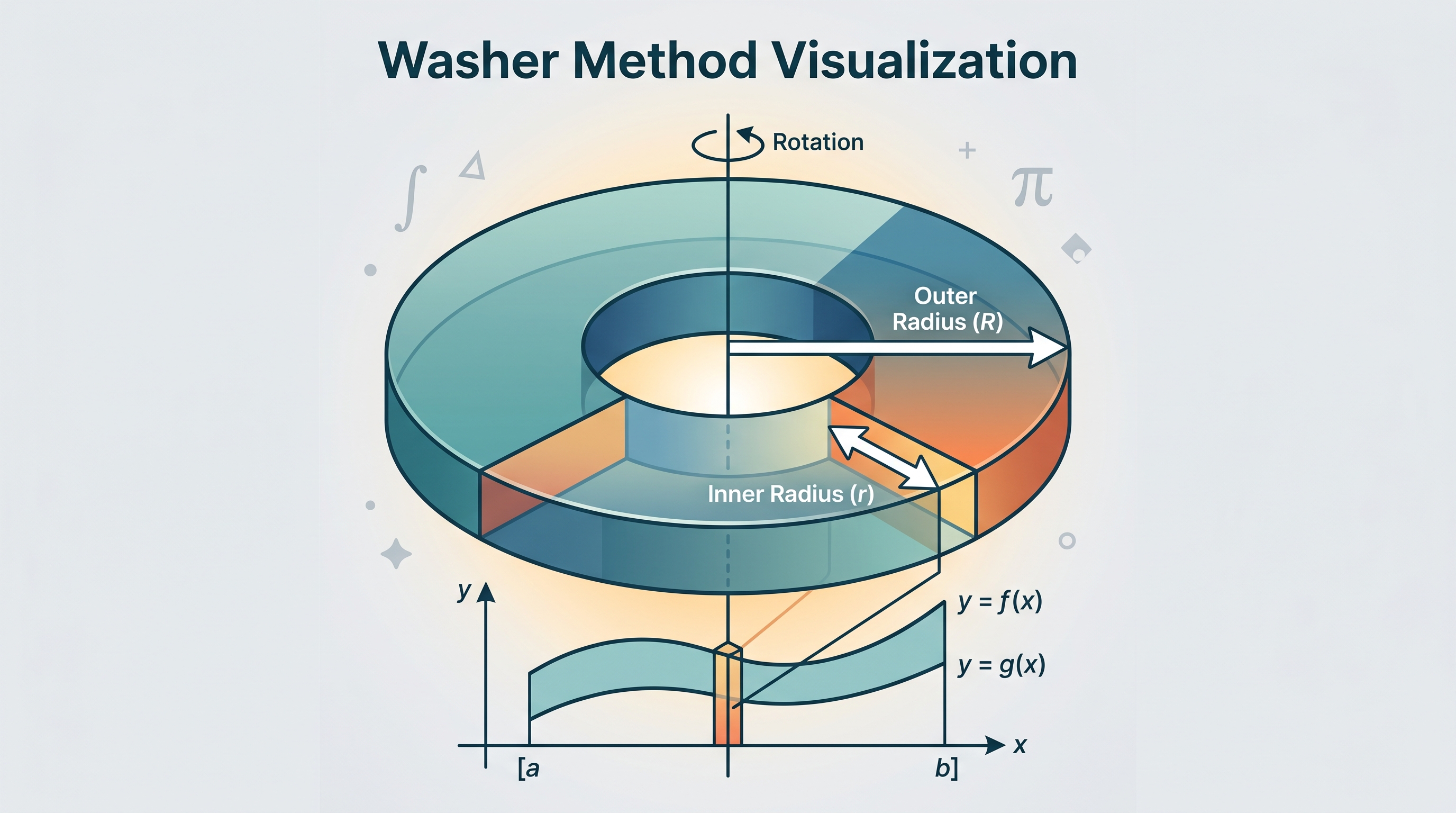
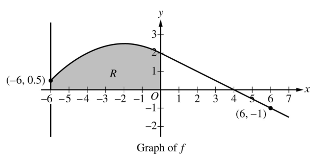
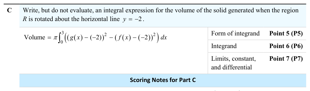
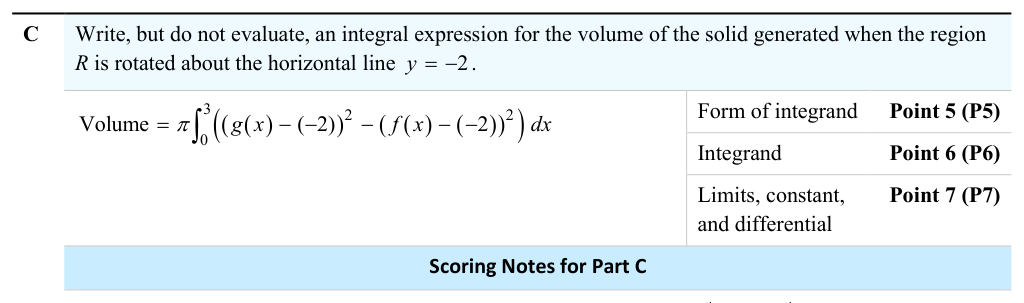
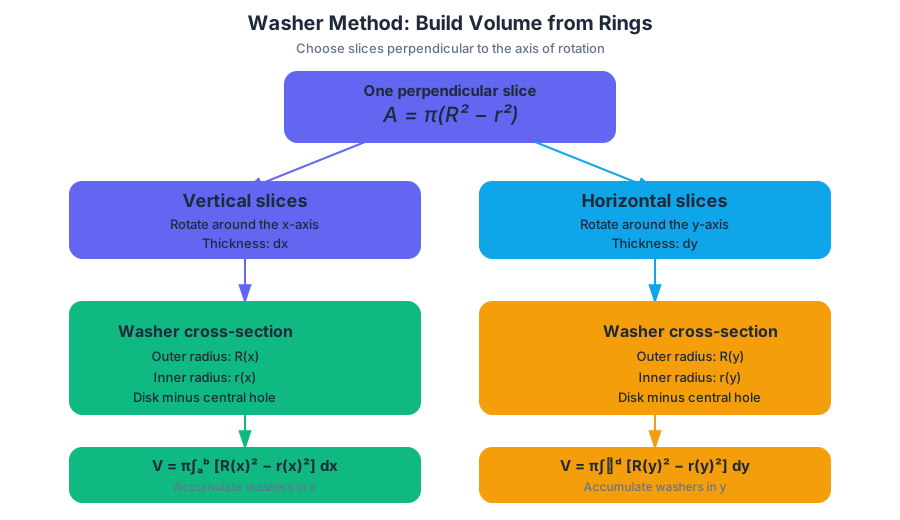
8.12 Volume with Washer Method: Revolving Around Other Axes
Key concepts: Washer method for finding volumes of solids of revolution · Disk and washer cross sections as ring-shaped regions · Volumes of revolution around horizontal or vertical lines other than the coordinate axes · Using definite integrals to represent volume · Determining outer and inner radii from distances to the line of revolution · Formula V = π∫(R^2 - r^2) for washer volumes · Connecting a geometric solid to its integral representation · Applying appropriate rounding procedures · Choosing the correct setup when the axis of rotation is shifted
How to set up washer-method volumes when the axis of rotation is a shifted line such as y = k or x = h, measuring both radii as distances to that line.
8.12 Volume with Washer Method: Revolving Around Other Axes
Topic 8.11 revolved regions around the $x$- or $y$-axis, where each radius could be read from a function value. When the axis of rotation is another horizontal or vertical line, such as $y=-2$ or $y=20$, the washer formula does not change, but $R$ and $r$ must both be measured from that line.
Washer area:
$$A=\pi\left(R^2-r^2\right)$$
Here, $R$ is the outer radius and $r$ is the inner radius.
The washer method accumulates these cross-sectional areas with a definite integral. If vertical slices are used, the volume is
$$V=\pi\int_a^b\left[R(x)^2-r(x)^2\right],dx.$$
For horizontal slices, the corresponding form is
$$V=\pi\int_c^d\left[R(y)^2-r(y)^2\right],dy.$$
The variable of integration is determined by the direction of the slices, not merely by the appearance of the functions.
A slice must be perpendicular to the axis of rotation. Rotation about a horizontal line produces washers from vertical slices, so the integral is usually written with respect to $x$. Rotation about a vertical line produces washers from horizontal slices, so the integral is usually written with respect to $y$.
For rotation around the coordinate axes, radii are measured from the appropriate axis:
- Around the $x$-axis, a vertical distance in $y$ becomes a radius.
- Around the $y$-axis, a horizontal distance in $x$ becomes a radius.
- Around a shifted horizontal line $y=k$, radius means vertical distance $\lvert y-k\rvert$.
- Around a shifted vertical line $x=h$, radius means horizontal distance $\lvert x-h\rvert$.
The crucial question is always: Which boundary is farther from the line of revolution?
Worked example: a shifted horizontal axis
Consider the region bounded by
$$y=\sqrt{x},\qquad y=0,\qquad x=0,\qquad x=4,$$
rotated about the horizontal line $y=-2$.
A representative vertical rectangle has thickness $dx$. When rotated around $y=-2$, it forms a washer. For $x>0$, the upper edge at $y=\sqrt{x}$ is farther from $y=-2$ than the lower edge at $y=0$. Therefore,
$$R(x)=\sqrt{x}+2,\qquad r(x)=2.$$
The cross-sectional area is
$$A(x)=\pi\left[(\sqrt{x}+2)^2-2^2\right].$$
Thus the volume is
$$V=\pi\int_0^4\left[(\sqrt{x}+2)^2-4\right],dx.$$
Simplify the integrand:
$$ (\sqrt{x}+2)^2-4 =x+4\sqrt{x}+4-4 =x+4\sqrt{x}. $$
So
$$ \begin{aligned} V &=\pi\int_0^4\left(x+4x^{1/2}\right),dx\ &=\pi\left[\frac{x^2}{2}+\frac{8}{3}x^{3/2}\right]_0^4\ &=\pi\left(8+\frac{64}{3}\right)\ &=\frac{88\pi}{3}. \end{aligned} $$
Numerically,
$$V\approx 92.154\text{ cubic units}.$$
This example shows why the shifted axis changes the radii. If the same region were rotated about the $x$-axis, the distances would be measured from $y=0$, giving $R(x)=\sqrt{x}$ and $r(x)=0$. Moving the axis down to $y=-2$ changes both distances to $R(x)=\sqrt{x}+2$ and $r(x)=2$.
A radius is a distance, not automatically a function value
The expressions $R(x)$ and $r(x)$ must represent distances to the axis of rotation. For example, if a region between $y=f(x)$ and $y=g(x)$ is rotated about $y=20$, with $0\le g(x)\le f(x)\le20$, then
$$R(x)=20-g(x),\qquad r(x)=20-f(x).$$
The lower boundary is farther from $y=20$, even though $g(x)$ is the smaller function value. Comparing function heights alone can therefore produce the wrong radius assignment.
For an axis $y=k$, distances may require absolute values:
$$\text{distance from }y=u\text{ to }y=k=\lvert u-k\rvert.$$
If the region crosses the axis, the outer and inner boundaries may change, and the interval may need to be split where the geometry changes.
The AP skill 2.D — Connecting Representations appears when you connect the rectangle, its rotated washer, the radius functions, and the definite integral. The AP skill 4.E — Use appropriate mathematical symbols, notation, and language matters when you identify $R$, $r$, bounds, units, and a properly rounded numerical result.
Misconception check: The “outer” radius is not necessarily the larger function value. It is the larger distance to the rotation line.
Retrieval check: A region lies between $y=f(x)$ and $y=g(x)$ and rotates about $y=-2$, with $f(x)\ge g(x)\ge0$. Which setup is correct?
$$\pi\int_a^b\left[(f(x)+2)^2-(g(x)+2)^2\right],dx.$$
The reason is geometric: both radii are measured upward from $y=-2$, and the boundary farther from that line produces $R(x)$.
8.13 Arc Length of a Smooth, Planar Curve and Distance Traveled (BC only)
Key concepts: Arc length as the accumulation of infinitesimal changes in length over an interval · Arc length of a smooth planar curve represented as y=f(x) · Arc length of a parametrically represented curve · Particle speed as the magnitude of its velocity vector · Total distance traveled versus displacement · Using different representations to relate mathematical characteristics and properties · Specifying the interval and endpoints when setting up an arc-length integral
A curve can be much longer than the straight-line distance between its endpoints because every tiny turn contributes additional length. Arc length measures the accumulated length of a smooth planar path, while particle distance measures the accumulated magnitude of motion.
8.13 Arc Length of a Smooth, Planar Curve and Distance Traveled (BC only)
A curve can be much longer than the straight-line distance between its endpoints because every tiny turn contributes additional length. Arc length measures the accumulated length of a smooth planar path, while particle distance measures the accumulated magnitude of motion.
Enduring Understanding CHA-6: Definite integrals allow us to solve problems involving the accumulation of change in length over an interval.
From tiny line segments to arc length
Imagine replacing a curved path with many short straight segments. If one segment changes horizontally by $\Delta x$ and vertically by $\Delta y$, its length is approximately
$$ \sqrt{(\Delta x)^2+(\Delta y)^2}. $$
As the segments become infinitely short, their sum approaches the exact arc length. The definite integral performs this accumulation continuously.
Arc length when $y=f(x)$
For a smooth curve $y=f(x)$ on the interval $[a,b]$, the vertical change associated with a small horizontal change $dx$ is approximately $dy=f'(x),dx$. Substituting these changes into the distance formula gives
$$ ds=\sqrt{(dx)^2+(dy)^2} =\sqrt{1+\left(\frac{dy}{dx}\right)^2},dx. $$
Therefore, the arc length is
$$ \boxed{L=\int_a^b\sqrt{1+[f'(x)]^2},dx}. $$
The interval is part of the answer. Writing only
$$ \int\sqrt{1+[f'(x)]^2},dx $$
does not specify which portion of the curve is being measured.
Worked example: a rising cable
A cable follows the curve $y=x^2$ for $0\le x\le1$. Its derivative is $f'(x)=2x$, so the length is
$$ L=\int_0^1\sqrt{1+(2x)^2},dx =\int_0^1\sqrt{1+4x^2},dx. $$
This integral may require numerical evaluation. A calculator gives
$$ L\approx 1.479. $$
The horizontal distance is only $1$, and the vertical rise is also $1$; the curved cable is longer than either individual change.
Misconception check — “Arc length is just the integral of the derivative.” The integral $\int_a^b f'(x),dx$ gives net vertical change, not path length. Arc length requires the Pythagorean factor $\sqrt{1+[f'(x)]^2}$, which counts both horizontal and vertical changes.
Parametric curves: one formula for length and speed
When a curve is represented parametrically by
$$ x=x(t),\qquad y=y(t),\qquad a\le t\le b, $$
the changes over a small time interval are $dx=x'(t),dt$ and $dy=y'(t),dt$. Thus,
$$ \boxed{L=\int_a^b\sqrt{[x'(t)]^2+[y'(t)]^2},dt}. $$
The same expression has a motion interpretation. For a particle with position vector
$$ \mathbf r(t)=\langle x(t),y(t)\rangle, $$
the velocity vector is
$$ \mathbf v(t)=\langle x'(t),y'(t)\rangle, $$
and its speed, the magnitude of velocity, is
$$ \boxed{\text{speed}=\sqrt{[x'(t)]^2+[y'(t)]^2}}. $$
Consequently, total distance traveled from $t=a$ to $t=b$ is
$$ \boxed{D=\int_a^b\sqrt{[x'(t)]^2+[y'(t)]^2},dt}. $$
Distance traveled versus displacement
Displacement describes the net change from the initial position to the final position:
$$ \Delta\mathbf r=\mathbf r(b)-\mathbf r(a). $$
The magnitude of displacement is the straight-line distance between those two positions. Distance traveled follows the entire path and is therefore generally at least as large as the magnitude of displacement.
For example, let
$$ x(t)=t^2,\qquad y(t)=t,\qquad 0\le t\le1. $$
The particle begins at $(0,0)$ and ends at $(1,1)$, so
$$ |\Delta\mathbf r|=\sqrt{1^2+1^2}=\sqrt2. $$
Its speed is
$$ \sqrt{(2t)^2+1^2}=\sqrt{4t^2+1}, $$
so its total distance is
$$ D=\int_0^1\sqrt{4t^2+1},dt\approx1.479. $$
Thus $D\ne|\Delta\mathbf r|$.
Misconception check — “Integrating velocity gives distance.” Integrating the velocity vector gives displacement. Distance requires integrating speed, the nonnegative magnitude of velocity. In one-dimensional motion this distinction appears as
$$ \text{displacement}=\int_a^b v(t),dt, \qquad \text{distance}=\int_a^b |v(t)|,dt. $$
Recovering position from velocity
If velocity is known, position is recovered by integration. Suppose
$$ \mathbf v(t)=\langle 2t,1\rangle, \qquad \mathbf r(0)=\langle3,-2\rangle. $$
Integrating component by component gives
$$ \mathbf r(t)=\langle t^2+C_1,t+C_2\rangle. $$
Applying the initial-position condition $\mathbf r(0)=\langle3,-2\rangle$ yields $C_1=3$ and $C_2=-2$, so
$$ \mathbf r(t)=\langle t^2+3,t-2\rangle. $$
The initial condition is essential: velocity determines how position changes, but not the starting location.
Representations and AP skill connection
Topic 8.13 develops Suggested Skill 3.D: Apply an appropriate mathematical definition, theorem, or test by selecting the correct arc-length or distance formula and using the full interval. It also develops 2.D: Identify how mathematical characteristics or properties of functions are related in different representations: the graph shows the path, the parametric equations describe coordinates, derivatives give velocity, and the integral accumulates length.
Retrieval check: A particle travels from $t=0$ to $t=\pi$ with
$$ x(t)=\cos t,\qquad y(t)=\sin t. $$
Its speed is
$$ \sqrt{(-\sin t)^2+(\cos t)^2}=1, $$
so the distance traveled is
$$ \int_0^\pi1,dt=\pi. $$
The particle traces a semicircle of radius $1$, whose arc length is also $\pi$. What is the magnitude of its displacement? It is $2$, confirming that path length and displacement magnitude are different quantities.
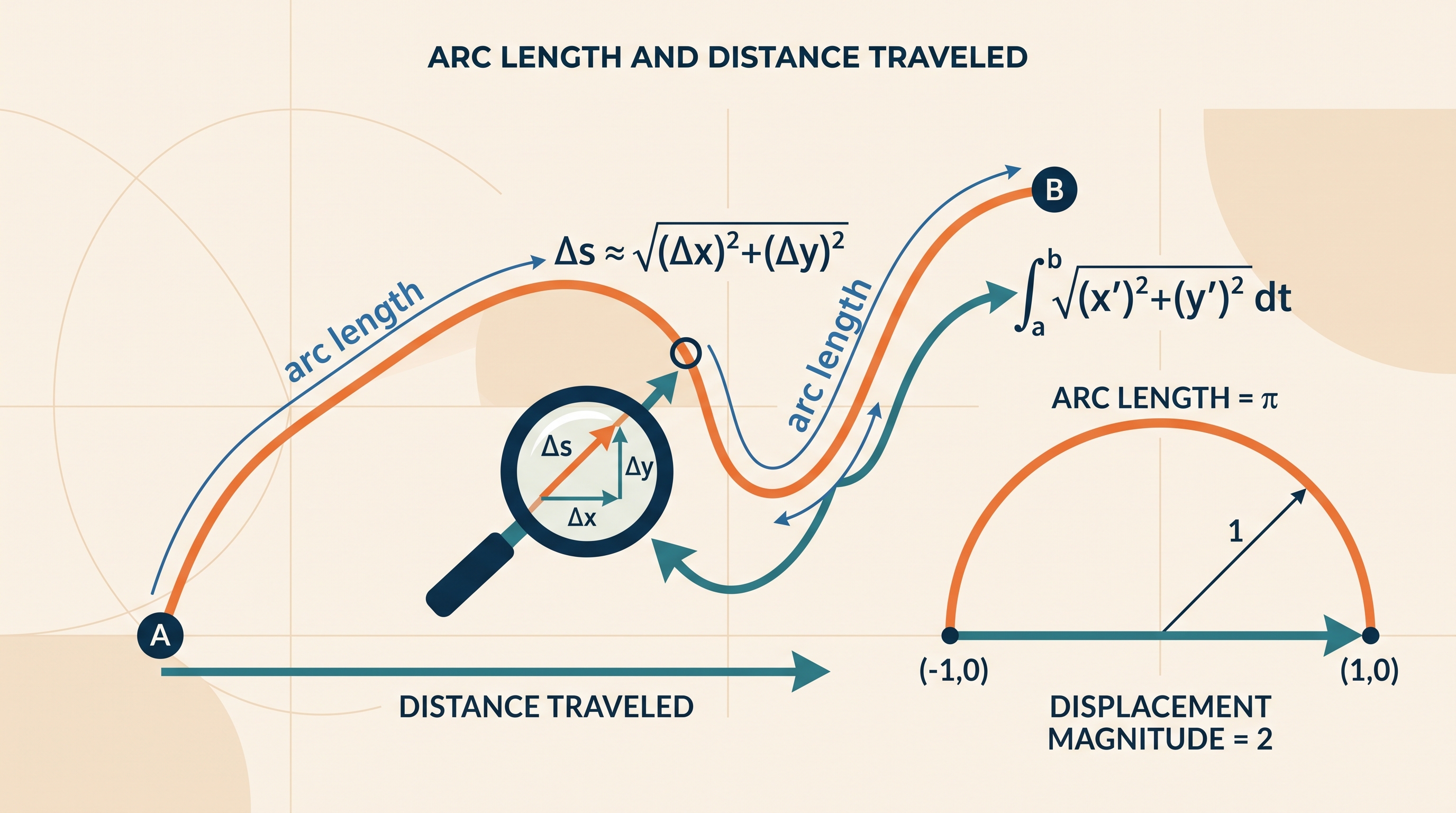
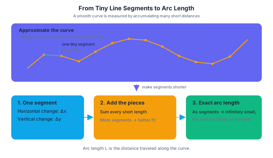
AP Practice 1
Key concepts: AP course requirements and the AP Course Audit · AP opposition to indoctrination and analysis of multiple perspectives · Respectful, evidence-based debate in AP classrooms · AP Exam scoring by trained college faculty and expert AP teachers · Combination of free-response/performance and computer-scored multiple-choice results · Conversion of raw scores into AP scores of 3, 4, or 5 · AP Reader compensation, travel expenses, and continuing education units · Writing limits in analytical form · Creating representations and comparing different limit expressions · Differentiation and contextual applications of differentiation, including particle motion in the plane
A limit must first be written as an analytical statement, not merely described in words or guessed from a graph. The precise form
AP Practice 1
A limit must first be written as an analytical statement, not merely described in words or guessed from a graph. The precise form
$$ \lim_{x\to x_0} f(x)=L $$
asserts that the values of $f(x)$ approach $L$ as $x$ approaches $x_0$—even if $f(x_0)$ is different from $L$ or does not exist.
This practice set focuses on the calculator-free task of writing, interpreting, and comparing limits. It also connects the mathematics to the larger AP system: authorized courses follow required curricular and resource conditions, classroom arguments rely on evidence rather than personal agreement, and free-response work is evaluated by trained AP Readers using published scoring criteria.
What makes an AP course—and what makes an AP response?
A school may label a course Advanced Placement or AP only after completing the AP Course Audit and satisfying the required curricular and resource expectations. For AP Calculus AB, those expectations include access to a college-level calculus textbook, coverage of the required Course and Exam Description content, opportunities to connect analytical, numerical, graphical, and verbal representations, mathematical justification and communication, graphing-calculator use, and applications of calculus to real-world situations.
The same evidence-centered habit governs classroom discussion. AP students are expected to analyze perspectives different from their own; points are awarded for mathematically correct reasoning, not for agreeing with a particular viewpoint. Students evaluate arguments and evidence—not one another—while respectful debate protects diverse backgrounds, experiences, and viewpoints. Personal attacks do not strengthen an argument and have no place in an AP classroom.
Unofficial calculator-free practice task
Timing guidance: Allow approximately $10$–$12$ minutes. Work without a graphing calculator. Write enough notation and explanation that another reader can follow the reasoning without reconstructing missing steps.
Let
$$ p(x)=\frac{x^2-9}{x-3} \qquad\text{for }x\ne 3. $$
Part A — Write the limit analytically
Write a limit statement that describes the value approached by $p(x)$ as $x$ approaches $3$. Then determine that limit.
Worked reasoning: Factor the numerator for values of $x$ near, but not equal to, $3$:
$$ p(x)=\frac{(x-3)(x+3)}{x-3}=x+3. $$
Therefore,
$$ \lim_{x\to 3}p(x)
\lim_{x\to 3}(x+3)
$$
Unofficial scoring guide, $2$ points: Award one point for the correct analytical form $\lim_{x\to 3}p(x)$ and one point for the correct value $6$. A response that writes only “the limit is $6$” gives the numerical result but does not fully display the required limiting relationship.
Key insight: The limit describes nearby behavior. It does not automatically equal the function’s value at the target input.
Part B — Compare two limit expressions
Compare the following expressions:
$$ \lim_{x\to 3}p(x) \qquad\text{and}\qquad p(3). $$
Are they necessarily equal for this function? Explain.
Worked reasoning: The formula for $p(x)$ is undefined at $x=3$ because its original denominator is zero. Thus $p(3)$ does not exist. However, the simplified expression $x+3$ describes the values of $p(x)$ for every nearby $x\ne3$, so
$$ \lim_{x\to3}p(x)=6 \qquad\text{while}\qquad p(3)\text{ is undefined}. $$
The two expressions are not equal because one exists as a limit and the other is not defined.
Unofficial scoring guide, $2$ points: Award one point for identifying the limit as $6$ and one point for explaining that $p(3)$ is undefined. Merely substituting $x=3$ into the unsimplified formula is not valid.
Part C — Relate one-sided and two-sided limits
Suppose a graph shows that
$$ \lim_{x\to 3^-}q(x)=5 \qquad\text{and}\qquad \lim_{x\to 3^+}q(x)=5. $$
What is $\lim_{x\to3}q(x)$? What conclusion would follow if the two one-sided limits were $5$ and $7$ instead?
Worked reasoning: A two-sided limit exists when the left-hand and right-hand limits agree. Since both one-sided limits equal $5$,
$$ \lim_{x\to3}q(x)=5. $$
If instead
$$ \lim_{x\to3^-}q(x)=5 \qquad\text{and}\qquad \lim_{x\to3^+}q(x)=7, $$
then the two-sided limit does not exist because the function approaches different values from the two sides.
Unofficial scoring guide, $2$ points: Award one point for the correct two-sided limit when the one-sided limits agree and one point for explaining nonexistence when they disagree.
How AP scoring works
On the AP Exam, multiple-choice responses are scored by machine, while free-response work is scored by trained AP Readers. These Readers include college faculty and expert AP teachers. Most scoring occurs during the annual AP Reading, with a smaller portion completed online. Readers receive compensation; traveling Readers have expenses, lodging, and meals covered, and Readers may earn continuing education units.
Free-response results are weighted and combined with computer-scored multiple-choice results to produce a raw score. That raw score is then converted into an AP score using standards for the reported scale, including scores of $3$, $4$, and $5$. The conversion is not simply a percentage grade, so a single missed point does not automatically determine the final AP score.
Retrieval check
Write the following claim in correct analytical form: “As $x$ approaches $2$, the function $r$ approaches $-4$.” Then state the condition required for a two-sided limit to exist.
Answer:
$$ \lim_{x\to2}r(x)=-4. $$
The left-hand and right-hand limits must both exist and equal the same number. The essential habit is to write the limit relationship first, then support it with comparison, algebra, a table, or a graph.
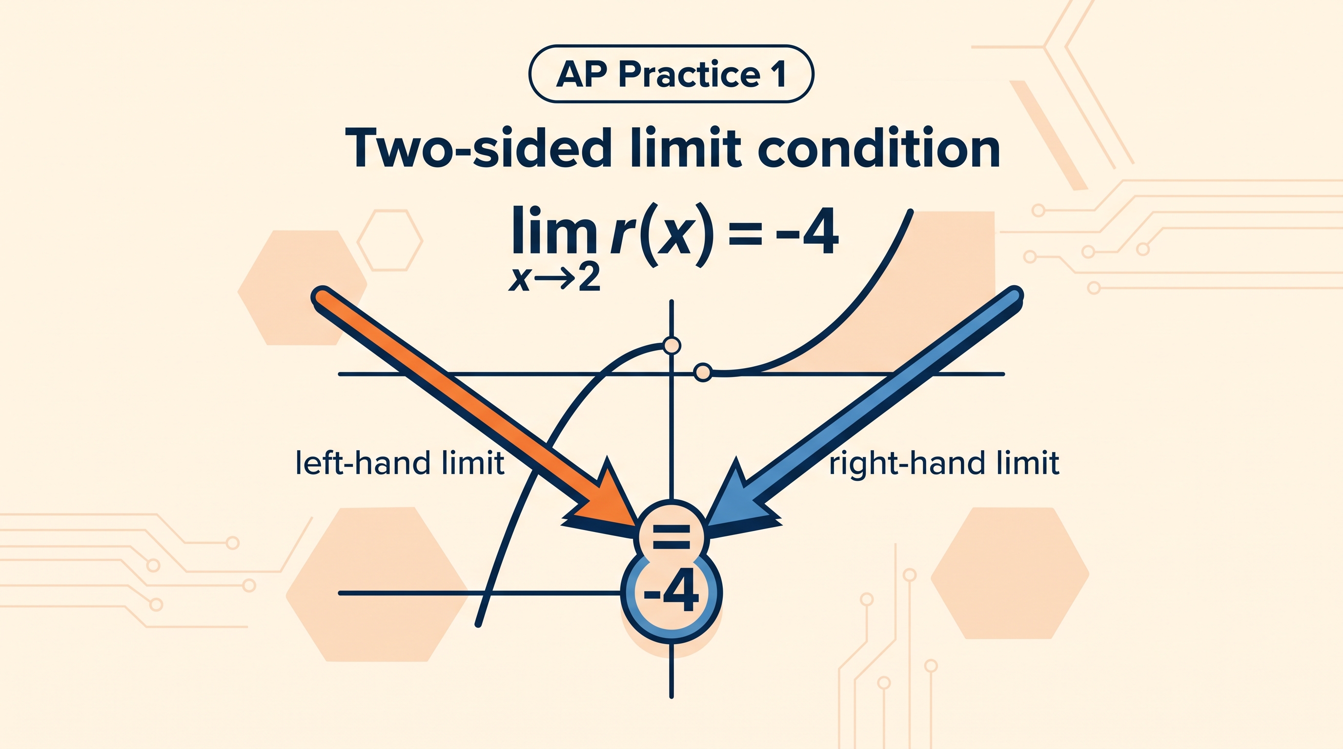
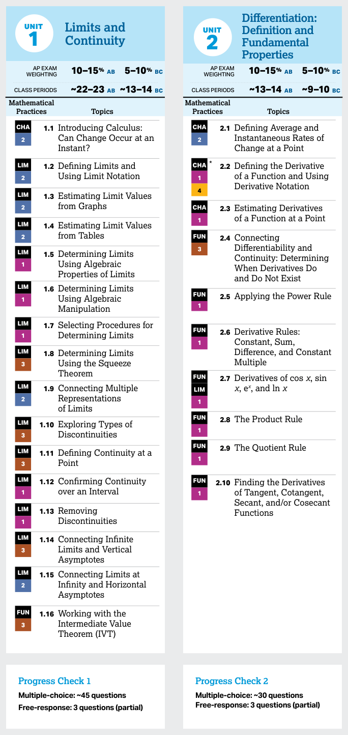
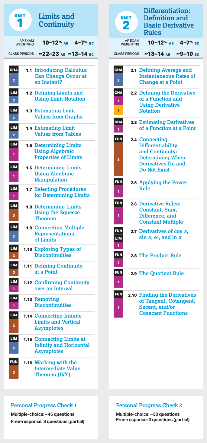
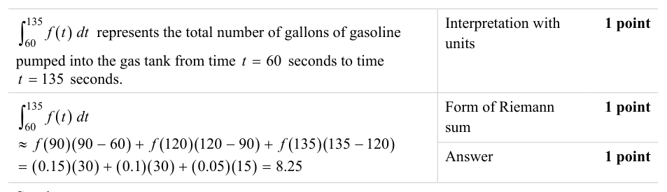
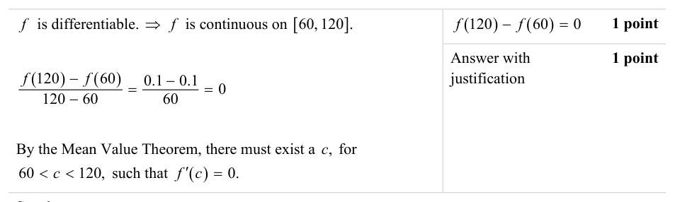
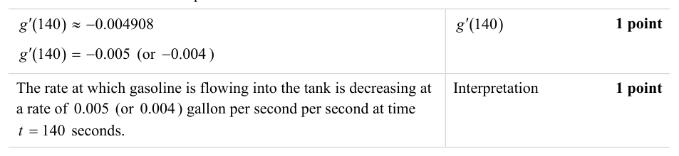

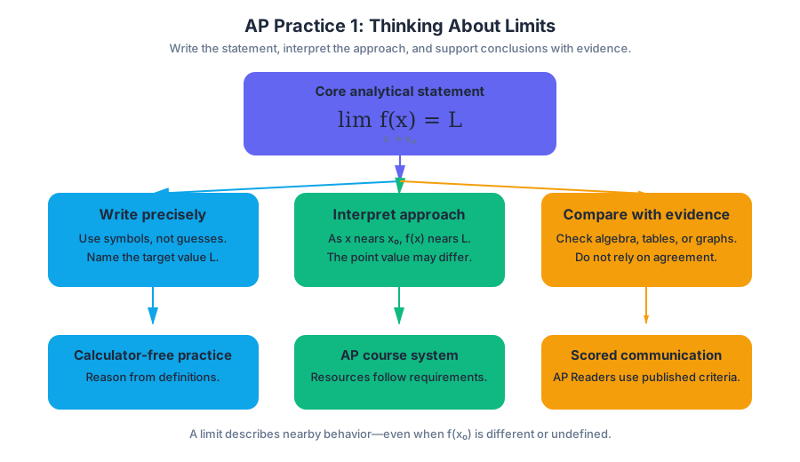
AP Practice 2
Key concepts: Translating among tabular, graphical, analytical, and verbal representations of functions · Continuity and differentiability at domain boundaries · Using the underlying context to decide between differentiation and integration · Exponential growth and decay models · Geometric and harmonic series, including alternating series · Predicting infinite totals through geometric-series models · Mathematical practices involving justification, communication, and notation · AP Calculus AB and BC multiple-choice exam structure · Differentiating composite trigonometric functions · Identifying values where a function is not differentiable
A strong calculus solution can move fluently between a table, graph, equation, and sentence without changing the underlying meaning. The same fluency also reveals which operation belongs: differentiation measures an instantaneous rate, while integration accumulates a rate over an interval.
AP Practice 2
A strong calculus solution can move fluently between a table, graph, equation, and sentence without changing the underlying meaning. The same fluency also reveals which operation belongs: differentiation measures an instantaneous rate, while integration accumulates a rate over an interval.
Exam map: where this practice belongs
For the current AP Calculus AB and BC exam format, Section I is multiple choice and contains two parts:
| Part | Calculator policy | Questions | Time |
|---|---|---|---|
| Section I, Part A | No calculator | $30$ | $60$ minutes |
| Section I, Part B | Graphing calculator permitted | $15$ | $45$ minutes |
Section II contains $6$ free-response questions completed in $90$ minutes. The first $2$ questions are calculator-active, and the remaining $4$ questions are calculator-inactive. AB students are assessed on the AB content; BC students encounter the AB content plus BC topics such as infinite series. In the multiple-choice section, Mathematical Practice 1: Implementing Mathematical Processes, Mathematical Practice 2: Connecting Representations, and Mathematical Practice 3: Justification are assessed; Mathematical Practice 4: Communication and Notation is not assessed there, although clear communication and notation matter especially in free response.
A useful pacing target is about $2$ minutes per question in no-calculator multiple choice and about $3$ minutes per question in calculator multiple choice. These are guides, not rigid rules: if a representation can be interpreted directly, do not spend calculator time performing algebra that the graph or table already answers.
Representation translation: one quantity, four languages
Suppose a tank’s water level is described by the sentence: “At time $t=3$ hours, the level is increasing at $4$ centimeters per hour.” The analytical representation is $h'(3)=4$, the verbal representation gives the units and meaning, a graph of $h$ has slope $4$ at $t=3$, and a table for $h$ would show nearby average slopes approaching $4$.
Worked question 1: read the table, then speak its meaning
A differentiable function $R$ gives a reading rate in words per minute. The table shows $R(0)=90$, $R(2)=100$, $R(8)=150$, and $R(10)=162$. Estimate $R'(1)$ using the available data.
$$ R'(1)\approx \frac{R(2)-R(0)}{2-0} =\frac{100-90}{2}=5. $$
The estimate is $5$ words per minute per minute. The calculation is an analytical representation, the table is numerical, and the final sentence is verbal. A complete response must not merely write $5$; it must identify what $5$ measures and include units.
Rewarded reasoning: connects the table to an average-rate approximation, identifies that the result estimates an instantaneous rate, and states appropriate units.
Misconception check — confusing $R(1)$ with $R'(1)$. The value $R(1)$ would be a reading rate. The value $R'(1)$ describes how that reading rate is changing. They have different meanings and different units.
Differentiation or integration? Let the context decide
Use differentiation when the question asks for a rate at a particular instant: velocity at $t=4$, the rate at which a population is changing, or the slope of a graph. Use integration when a rate is accumulated across an interval: total distance from velocity, total water entering from an inflow rate, or total words read from a reading-rate function.
Worked question 2: choose the operation before calculating
A machine produces items at a rate $p(t)$ items per hour. Which expression gives the total number of items produced from $t=2$ to $t=7$?
$$ \int_2^7 p(t),dt $$
The integral is correct because the problem asks for a total accumulated amount. By contrast, $p'(5)$ would measure how rapidly the production rate itself is changing at $t=5$.
Exponential growth and decay
A statement such as “the population increases at a rate proportional to its current population” translates into
$$ \frac{dP}{dt}=kP. $$
Its model is
$$ P(t)=P_0e^{kt}, $$
where $P_0$ is the initial population. If $k>0$, the model represents growth; if $k<0$, it represents decay.
Worked question 3: translate the rate statement
A chemical sample contains $80$ grams initially and decays at a rate proportional to the amount present, with proportionality constant $-0.25$. The model is
$$ \frac{dA}{dt}=-0.25A, \qquad A(t)=80e^{-0.25t}. $$
After $4$ hours,
$$ A(4)=80e^{-1}\approx 29.431. $$
The negative sign belongs in the differential equation because the amount is decreasing. Omitting it produces growth rather than decay.
Boundary behavior and differentiability
At an interior breakpoint, both sides matter. Consider
$$ f(x)= \begin{cases} x^2, & x\le 2,\ 4x-4, & x>2. \end{cases} $$
Here $x=2$ is an interior breakpoint, not a domain boundary, because the domain includes values both less than and greater than $2$.
The left-hand limit is
$$ \lim_{x\to2^-}f(x)=4, $$
and the right-hand limit is
$$ \lim_{x\to2^+}f(x)=4. $$
Since $f(2)=4$, the function is continuous at $x=2$. The one-sided derivatives are
$$ \lim_{x\to2^-}\frac{d}{dx}(x^2)=4, \qquad \lim_{x\to2^+}\frac{d}{dx}(4x-4)=4, $$
so $f$ is also differentiable at $x=2$.
At a genuine domain boundary, only the derivative from within the domain is relevant. For
$$ g(x)=\sqrt{x-1}, \qquad x\ge1, $$
the point $x=1$ is a domain boundary. Continuity uses the right-hand limit:
$$ \lim_{x\to1^+}\sqrt{x-1}=0=g(1). $$
A boundary derivative, when defined in the course’s one-sided sense, is tested using the right-hand difference quotient. There is no left-hand domain from which to approach.
Worked question 4: find where differentiability fails
For
$$ q(x)=|x-3|, $$
the function is continuous at $x=3$, but its left-hand slope is $-1$ and its right-hand slope is $1$. Because the one-sided derivatives disagree, $q$ is not differentiable at $x=3$.
Key distinction: differentiability implies continuity, but continuity does not imply differentiability.
Infinite totals and series
If a repeatedly distributed piece is always a fixed fraction $r$ of the previous piece, the total is modeled by a geometric series:
$$ a+ar+ar^2+ar^3+\cdots. $$
When $|r|<1$, the infinite total is
$$ \sum_{n=0}^{\infty}ar^n=\frac{a}{1-r}. $$
For example, if a $12$-inch strip of licorice is divided so that each next piece is $\frac13$ of the previous piece, then the predicted total represented by all pieces is
$$ 12\left(1+\frac13+\frac19+\cdots\right) =\frac{12}{1-\frac13}=18\text{ inches}. $$
A harmonic series has terms such as
$$ \sum_{n=1}^{\infty}\frac1n $$
and diverges, meaning its partial sums grow without a finite limit. An alternating series changes signs, such as
$$ \sum_{n=1}^{\infty}(-1)^{n+1}\frac1n. $$
This alternating harmonic series converges even though the corresponding positive harmonic series diverges. These series topics are BC content.
Worked question 5: predict the infinite total
A donut is divided so that the first recipient receives $10$ units, the second receives $\frac12$ as much, and every later recipient receives half as much as the previous recipient. The total eventually distributed is
$$ \sum_{n=0}^{\infty}10\left(\frac12\right)^n =\frac{10}{1-\frac12}=20. $$
The model works because the common ratio satisfies $|r|<1$.
Mixed practice: choose, translate, justify
Question 6. Let $s(x)=\sin(4x)$. Which statement is correct?
A. $s'(x)=\cos(4x)$
B. $s'(x)=4\cos(4x)$
C. $s'(x)=\sin(4)$
D. $s'(x)=4\sin(x)$
The correct answer is B, because the outer derivative gives $\cos(4x)$ and the inner derivative of $4x$ gives $4$:
$$ \frac{d}{dx}\sin(4x)=\cos(4x)\cdot4=4\cos(4x). $$
Error-review routine: For each missed item, label the error as one of four types: representation translation, operation selection, boundary reasoning, or series/model interpretation. Then rewrite the answer in a complete sentence with units or conditions. For free response, preserve the chain of reasoning: equation, substitution or theorem condition, result, and interpretation. That practice develops Mathematical Practice 1: Implementing Mathematical Processes, Mathematical Practice 2: Connecting Representations, and Mathematical Practice 3: Justification, while strengthening the communication expected across roughly $10%$ to $25%$ of indicated assessment emphasis.
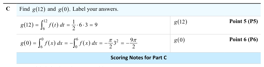
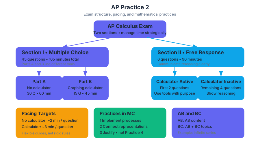
AP Practice 3
A graphing-calculator free-response question can ask you to move among a table, a rate function, an accumulation function, and a verbal conclusion—all while keeping units and justification visible.
AP Practice 3
A graphing-calculator free-response question can ask you to move among a table, a rate function, an accumulation function, and a verbal conclusion—all while keeping units and justification visible. The strongest response is not merely a collection of correct numbers: it shows a mathematically defensible chain from representation to conclusion.
Task type: calculator-active free-response question
Status: original and unofficial practice
Suggested time: $15$–$20$ minutes
The situation: water entering a reservoir
Water flows into a reservoir at a rate modeled by
$$ R(t)=\frac{180t}{t^2+9} $$
where $t$ is measured in hours and $R(t)$ is measured in liters per hour. At time $t=0$, the reservoir contains $420$ liters of water. A small outlet removes water at a constant rate of $8$ liters per hour.
Let $V(t)$ represent the volume of water in the reservoir, in liters, at time $t$.
(a) Write an expression involving an integral that gives the volume of water in the reservoir at time $t$.
(b) Find the rate at which the volume is changing at time $t=6$. Interpret your answer, including units.
(c) Determine the time $t$ in the interval $0\le t\le 10$ at which the volume is increasing most rapidly. Justify your answer.
(d) Find the average volume of water in the reservoir over the interval $0\le t\le 10$.
(e) A safety sensor activates whenever the volume reaches $600$ liters. Determine whether the sensor activates during the first $10$ hours. Justify your answer.
Part (a): Build the accumulation model
The net rate of change of volume is inflow minus outflow:
$$ V'(t)=R(t)-8=\frac{180t}{t^2+9}-8. $$
Starting with $420$ liters and accumulating the net change from $0$ to $t$ gives
$$ \boxed{V(t)=420+\int_0^t\left(\frac{180x}{x^2+9}-8\right),dx}. $$
The variable of integration is written as $x$ rather than $t$ because $t$ is the endpoint being evaluated. This distinction prevents the expression from confusing the input time with the temporary accumulation variable.
Rewardable reasoning: The response identifies the initial amount and adds the integral of the net rate. Writing only $\int_0^t R(x),dx$ omits the outlet and does not model the reservoir.
Part (b): Interpret a derivative in context
Evaluate the net rate at $t=6$:
$$ V'(6)=\frac{180(6)}{6^2+9}-8 =\frac{1080}{45}-8 =24-8 =16. $$
Therefore,
$$ \boxed{V'(6)=16\text{ liters per hour}}. $$
At time $t=6$ hours, the volume of water is increasing at an instantaneous rate of $16$ liters per hour.
Interpretation rule: A derivative in context must include what is changing, how quickly it is changing, and the appropriate units.
Part (c): Find when the volume increases most rapidly
Because $V'(t)$ is the rate at which volume changes, the volume increases most rapidly when $V'(t)$ is largest. Use the calculator to maximize
$$ V'(t)=\frac{180t}{t^2+9}-8 $$
on $0\le t\le 10$.
The maximum occurs at
$$ t=3. $$
Indeed, the variable part $\dfrac{180t}{t^2+9}$ reaches its maximum when $t=3$, giving
$$ V'(3)=\frac{180(3)}{3^2+9}-8 =\frac{540}{18}-8 =22. $$
Thus,
$$ \boxed{t=3\text{ hours}}. $$
A justification must connect the quantity being optimized to the question: maximizing $V(t)$ would find when the reservoir is fullest, not when it is filling fastest. A calculator-produced time without identifying the function being maximized is weaker mathematical communication.
Part (d): Average value of the volume
The average value of $V$ on $[0,10]$ is
$$ \frac{1}{10-0}\int_0^{10}V(t),dt =\frac{1}{10}\int_0^{10} \left[ 420+\int_0^t\left(\frac{180x}{x^2+9}-8\right),dx \right]dt. $$
Using a graphing calculator,
$$ \boxed{\frac{1}{10}\int_0^{10}V(t),dt\approx 676.1\text{ liters}}. $$
The average volume is not $V(5)$. The value $V(5)$ describes the reservoir at the midpoint in time; the average value accounts for the entire volume curve over the interval.
Part (e): Does the sensor activate?
To decide whether the volume reaches $600$ liters, examine the maximum value of $V(t)$ on $[0,10]$. Critical points occur where
$$ V'(t)=0. $$
Solving numerically gives
$$ t\approx 0.46 \quad\text{and}\quad t\approx 19.54. $$
Only $t\approx0.46$ lies in the interval $[0,10]$. Evaluate $V$ at the endpoints and the interior critical point:
$$ V(0)=420, $$
$$ V(0.46)\approx 424.8, $$
$$ V(10)\approx 735.9. $$
The largest volume during the first $10$ hours is approximately $735.9$ liters, which exceeds $600$ liters. Therefore,
$$ \boxed{\text{The safety sensor does activate during the first }10\text{ hours}.} $$
The conclusion is supported by an extreme-value check rather than by testing one convenient time. Since $V(10)>600$, the sensor definitely activates by $t=10$; continuity of $V$ guarantees that the volume must pass through $600$ on the way from below to above that value.
What an examiner rewards
| Mathematical Practice | Evidence in this response |
|---|---|
| Mathematical Practice 1: Implementing Mathematical Processes | Forms the net rate, writes accumulation and average-value integrals, and uses numerical procedures appropriately. |
| Mathematical Practice 2: Connecting Representations | Connects the verbal reservoir model to $V'(t)$, $V(t)$, integrals, and calculator-based numerical values. |
| Mathematical Practice 3: Justification | Explains why maximizing $V'(t)$ answers part (c) and why endpoint/critical-point analysis answers part (e). |
| Mathematical Practice 4: Communication and Notation | Uses defined variables, correct integral notation, contextual conclusions, and units. |
A response that reports calculator output without an equation, interpretation, or justification may earn less credit than a response with a small numerical error but a coherent method. In particular, preserve the distinction between a rate, an accumulated amount, and an average value.
Timing and error review
Spend approximately $3$ minutes modeling, $4$ minutes on derivative interpretation and maximization, $5$ minutes on average value, and $5$ minutes on the sensor decision. Afterward, label each error as one of four types: modeling, calculator setup, reasoning/justification, or notation and units. Then redo only the failed step without looking at the solution.
Retrieval check: If the outlet rate changed from $8$ liters per hour to $12$ liters per hour, which expression would change first—$V(t)$, $V'(t)$, or both? Explain why.
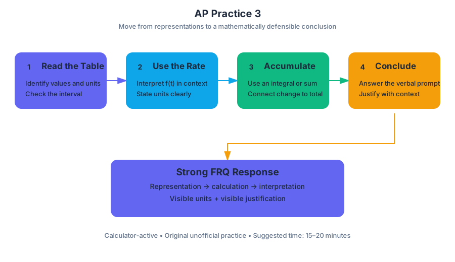
AP Practice 4
A rate can describe either a change averaged over time or a change occurring at one exact instant. The distinction matters when a tank, population, bank account, or chemical concentration is changing continuously.
AP Practice 4
A rate can describe either a change averaged over time or a change occurring at one exact instant. The distinction matters when a tank, population, bank account, or chemical concentration is changing continuously.
Task type: Calculator-active contextual free response
A water-treatment tank receives water at rate $I(t)$ gallons per hour and drains water at rate $D'(t)$ gallons per hour, where $t$ is measured in hours after 8:00 a.m. The function $D(t)$ gives the total number of gallons drained by time $t$. Values of $D(t)$ are recorded below.
| $t$ | $0$ | $2$ | $4$ | $5$ | $6$ | $8$ |
|---|---|---|---|---|---|---|
| $D(t)$ | $0$ | $430$ | $1{,}200$ | $1{,}440$ | $1{,}690$ | $2{,}100$ |
At exactly $t=5$, the drainage rate is known to be $D'(5)=240$ gallons per hour. The inflow rate at that moment is $I(5)=500$ gallons per hour. Let $V(t)$ represent the amount of water in the tank.
The questions
(a) Find the average rate at which water is drained from the tank over the interval $4\leq t\leq 8$. Include units.
(b) Interpret the meaning of $D'(5)=240$ in the context of the tank.
(c) Find $V'(5)$, the instantaneous rate of change of the amount of water in the tank at $t=5$. Include units.
(d) Is the amount of water in the tank increasing or decreasing at $t=5$? Justify your answer.
Worked solution
Part (a): Average rate from a table
An average rate of change uses two endpoint values:
$$ \text{average rate}
\frac{D(8)-D(4)}{8-4}. $$
Substitute the data from the table:
$$ \frac{2{,}100-1{,}200}{8-4}
\frac{900}{4}
$$
Therefore, the average drainage rate over $4\leq t\leq 8$ is
$$ \boxed{225\text{ gallons per hour}}. $$
The denominator is measured in hours, so the units are gallons per hour. This value describes the entire four-hour interval; it does not claim that the drainage rate was exactly $225$ gallons per hour at every instant.
Part (b): Meaning of a derivative
The derivative $D'(5)$ gives the instantaneous rate of change of the cumulative drained amount at the precise moment $t=5$. Thus,
$$ D'(5)=240 $$
means that, at $1:00$ p.m., water is leaving the tank at an instantaneous rate of $240$ gallons per hour.
A complete contextual response identifies the quantity, the time, the direction, and the units:
At $1:00$ p.m., the total amount of water drained is increasing at a rate of $240$ gallons per hour.
Part (c): Net rate of change
The amount in the tank increases because of inflow and decreases because of drainage. The rate equation is therefore
$$ V'(t)=I(t)-D'(t). $$
At $t=5$,
$$ V'(5)=I(5)-D'(5) =500-240 =260. $$
Hence,
$$ \boxed{V'(5)=260\text{ gallons per hour}}. $$
The value $D'(5)=240$ is supplied directly, so no estimate from the table is needed. The table can estimate an average drainage rate, but it cannot by itself determine the exact instantaneous value $D'(5)$.
Part (d): Increasing or decreasing?
Because
$$ V'(5)=260>0, $$
the amount of water in the tank is increasing at $t=5$. The inflow exceeds the drainage rate by $260$ gallons per hour.
$$ \boxed{\text{The amount of water is increasing at }t=5.} $$
What earns credit
This task combines the AP Mathematical Practices:
- Mathematical Practice 1: Implementing Mathematical Processes — compute an average rate and apply the net-rate equation.
- Mathematical Practice 2: Connecting Representations — move from a numerical table and derivative value to a contextual statement about the tank.
- Mathematical Practice 3: Justification — use the sign of $V'(5)$ to support the increasing/decreasing conclusion.
- Mathematical Practice 4: Communication and Notation — state units, identify the time, and distinguish $D(t)$ from $D'(t)$.
A strong response does not receive full reasoning credit for writing only $260$. It must show the relationship
$$ V'(5)=I(5)-D'(5) $$
and explain what the positive result means.
Misconception check
Average-versus-instantaneous confusion: Using
$$ \frac{D(8)-D(4)}{8-4}=225 $$
as though it were $D'(5)$ is invalid. The number $225$ summarizes the interval from $t=4$ to $t=8$; the exact instantaneous rate at $t=5$ is the separately provided value $D'(5)=240$.
Sign error in a net rate: Since drainage removes water, it must be subtracted:
$$ \text{net change}=\text{inflow}-\text{outflow}. $$
Writing $500+240$ would incorrectly treat drainage as an addition to the tank.
Timing and error review
Allow about $12$–$15$ minutes for the four parts. On review, label each line as one of three types: quantity, calculation, or interpretation. If an answer lacks units, a sign explanation, or a contextual sentence, repair that communication even when the numerical work is correct.
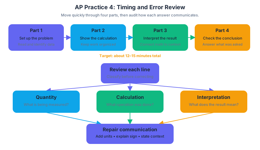
AP Practice 5
A pump’s changing flow rate can be analyzed in four representations at once: a table of measurements, a polynomial model, a derivative, and a definite integral.
AP Practice 5
A pump’s changing flow rate can be analyzed in four representations at once: a table of measurements, a polynomial model, a derivative, and a definite integral. This practice targets an original calculator-allowed free-response question, where correct procedures matter—but so do interpretation, justification, and notation.
Task profile
| Feature | Guidance |
|---|---|
| Task type | Calculator-allowed free-response question |
| Suggested time | About $15$ minutes |
| Main skills | Mathematical Practice 1: Implementing Mathematical Processes; Mathematical Practice 2: Connecting Representations; Mathematical Practice 3: Justification; Mathematical Practice 4: Communication and Notation |
| Typical evidence | Numerical derivative, definite integral, equation solving, units, and contextual conclusions |
| Calculator role | Numerical differentiation, integration, graphing, and solving are appropriate, but the mathematical setup must still be visible |
Original practice problem
Water flows through a treatment plant’s pump at a rate $R(t)$ liters per minute, where $t$ is measured in minutes. The pump begins operating at $t=10$. Measurements of the rate are shown below.
| $t$ | $10$ | $12$ | $15$ | $20$ | $25$ | $30$ |
|---|---|---|---|---|---|---|
| $R(t)$ | $20.0$ | $19.0$ | $17.6$ | $15.5$ | $13.6$ | $12.0$ |
For this problem, the plant uses the model
$$ R(t)=20-0.5(t-10)+0.005(t-10)^2 $$
for $10\le t\le 30$.
(a) Use the table to estimate $R'(15)$. Interpret your answer in context.
(b) Find the total amount of water pumped from $t=10$ to $t=20$.
(c) Find the average pumping rate on the interval $10\le t\le 20$.
(d) The pump is turned off when its rate first decreases to $14$ liters per minute after $t=10$. Find the time when the pump is turned off.
(e) Is the average pumping rate from $t=10$ until the pump is turned off greater than $17$ liters per minute? Justify your answer.
Worked solution
Part (a): Connect the table to a derivative
A centered difference around $t=15$ uses the closest available times on either side:
$$ R'(15)\approx \frac{R(20)-R(12)}{20-12} =\frac{15.5-19.0}{8} =-0.4375. $$
Therefore,
$$ R'(15)\approx -0.44\text{ liters per minute per minute}. $$
The negative sign means that at $t=15$, the pumping rate is decreasing by approximately $0.44$ liters per minute each minute.
Rubric-aligned evidence: The response earns the process credit by using a valid difference quotient, and it earns interpretation credit by explaining both the sign and the units. Writing only $-0.44$ is not a complete contextual answer.
Part (b): Accumulation through a definite integral
Because $R(t)$ is a rate in liters per minute, integrating it over a time interval gives an amount in liters:
$$ \text{Water pumped}=\int_{10}^{20}R(t),dt. $$
Using the model,
$$ \int_{10}^{20}\left[20-0.5(t-10)+0.005(t-10)^2\right]dt \approx 176.67. $$
The total amount pumped is therefore approximately
$$ \boxed{176.67\text{ liters}}. $$
A calculator may evaluate the integral, but the setup must show the correct rate function and bounds.
Part (c): Average value of a rate
The average pumping rate is not the total amount. It is the accumulated amount divided by elapsed time:
$$ R_{\text{avg}} =\frac{1}{20-10}\int_{10}^{20}R(t),dt =\frac{176.67}{10} \approx 17.67. $$
Thus the average pumping rate is
$$ \boxed{17.67\text{ liters per minute}}. $$
Part (d): First time the rate reaches $14$
Set the model equal to the shutdown rate:
$$ 20-0.5(t-10)+0.005(t-10)^2=14. $$
A numerical solver gives
$$ t\approx 22.55 $$
as the first solution after $t=10$. The pump is turned off at approximately
$$ \boxed{t=22.55\text{ minutes}}. $$
The model is decreasing on the relevant interval because
$$ R'(t)=-0.5+0.01(t-10), $$
and $R'(t)<0$ for $10\le t\le30$. Therefore, the first solution is the physically relevant shutdown time.
Part (e): Compare the average rate with $17$
Let $t_*=22.55$ be the shutdown time. The average rate from startup until shutdown is
$$ \frac{1}{t_-10}\int_{10}^{t_}R(t),dt \approx 17.13\text{ liters per minute}. $$
Since
$$ 17.13>17, $$
the average pumping rate is greater than $17$ liters per minute.
A complete conclusion states the comparison and refers to the calculated quantity: “Yes; the average rate is approximately $17.13$ liters per minute, which is greater than $17$ liters per minute.”
Common misconceptions
Confusing $R(t)$ with $R'(t)$. The function $R(t)$ measures water flow; its derivative measures how quickly that flow rate changes. Their units are different.
Forgetting the factor in an average value. The integral gives total water, not average rate. Divide by the interval length.
Using inconsistent models. The table and polynomial here describe the same rate pattern: the polynomial gives approximately $R(12)=19.02$, $R(15)=17.625$, and $R(20)=15.5$, matching the displayed rounded data.
Reporting a calculator output without justification. A numerical answer is strongest when accompanied by the equation, integral, or derivative expression that produced it.
Error-review routine
After completing the problem, label each error as one of four types: procedure, representation, justification, or communication and notation. Rework only the failed step, then check units and whether every requested contextual conclusion includes a sentence—not merely a number.
Retrieval check: If $R(t)$ is measured in liters per minute, what units must $\int_a^bR(t),dt$ have, and what units must $R'(t)$ have?
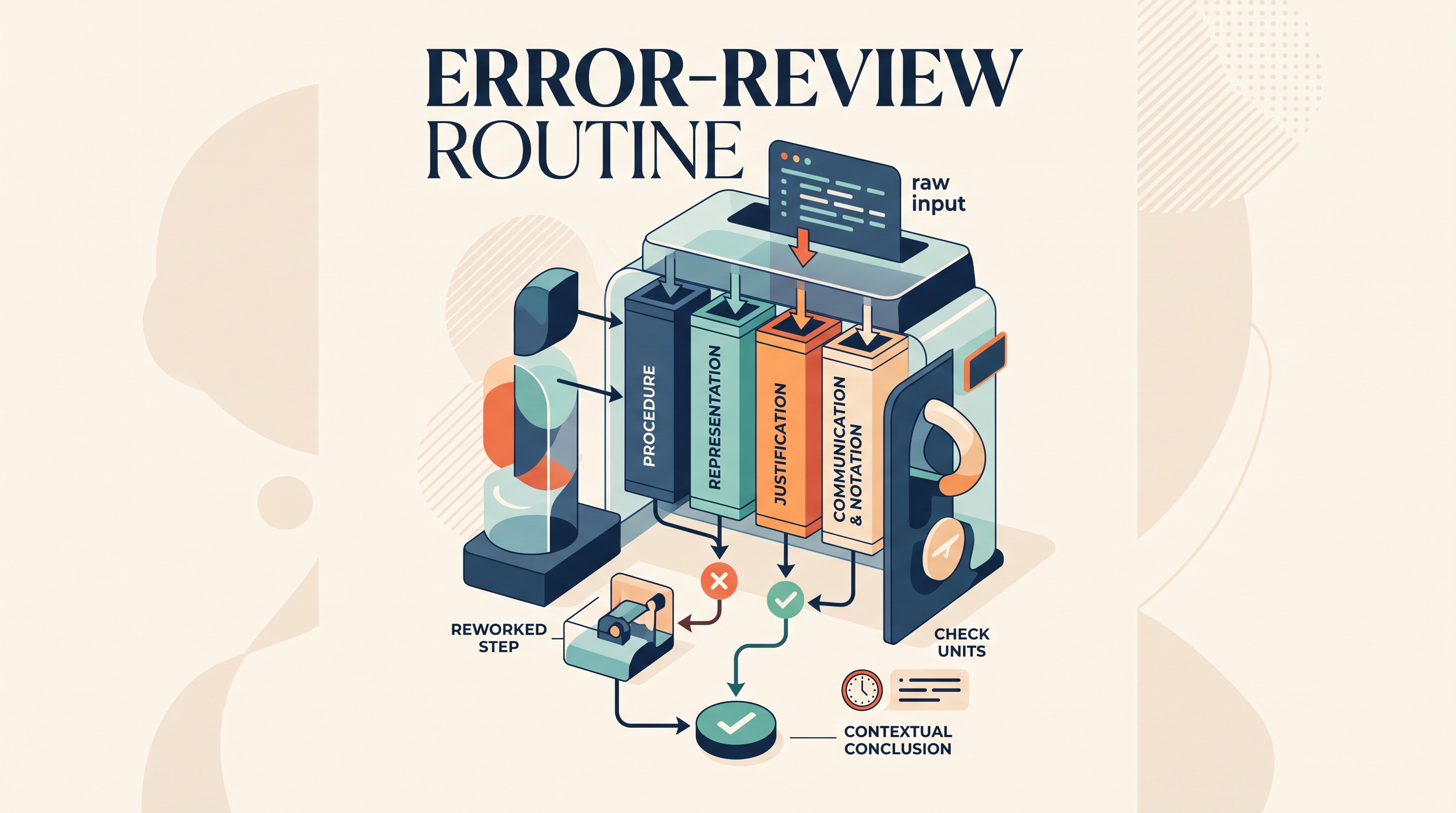
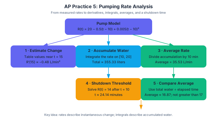
AP Practice 6
A water-treatment plant monitors the rate at which clean water enters a storage tank. The rate changes throughout the day, so the plant must combine a graph, numerical data, a derivative, and an accumulation model to answer one practical question: How much water is in the tank, and when is its level changing fastest?
AP Practice 6
A water-treatment plant monitors the rate at which clean water enters a storage tank. The rate changes throughout the day, so the plant must combine a graph, numerical data, a derivative, and an accumulation model to answer one practical question: How much water is in the tank, and when is its level changing fastest?
This practice is an original, unofficial calculator-active free-response task. It emphasizes the four Mathematical Practices: Mathematical Practice 1: Implementing Mathematical Processes, Mathematical Practice 2: Connecting Representations, Mathematical Practice 3: Justification, and Mathematical Practice 4: Communication and Notation.
Original practice task
Let $r(t)$ be the rate, in liters per minute, at which water enters a tank $t$ minutes after noon. The function $r$ is twice differentiable on the interval $0\leq t\leq 60$. At noon, the tank contains $420$ liters. Selected values of $r$ are shown below.
| $t$ | $0$ | $15$ | $30$ | $45$ | $60$ |
|---|---|---|---|---|---|
| $r(t)$ | $8.0$ | $11.5$ | $13.0$ | $10.0$ | $6.5$ |
Define the amount of water in the tank by
$$ W(t)=420+\int_0^t r(x),dx. $$
(a) Use the data table and the trapezoidal rule with four subintervals to approximate $W(60)$. Include units.
(b) Explain the meaning of $W'(30)$ in context and determine its value.
(c) The plant begins releasing water at a rate of $q(t)=0.1t$ liters per minute for $0\leq t\leq 60$. Let $N(t)$ represent the net rate of change of water in the tank. Write an expression for $N(t)$ and explain why the tank contains more water at $t=60$ than at noon.
(d) A sensor records that $r(20)=12.4$ and $r(40)=11.2$. Explain why there must be at least one time $c$ between $20$ and $40$ at which $r'(c)=0$.
Worked solution
Part (a): Accumulating a rate
The trapezoidal rule estimates the accumulated amount entering the tank:
$$ \int_0^{60}r(t),dt \approx \frac{15}{2}\left[r(0)+2r(15)+2r(30)+2r(45)+r(60)\right]. $$
Substitute the recorded values:
$$ \int_0^{60}r(t),dt \approx \frac{15}{2}\left[8.0+2(11.5)+2(13.0)+2(10.0)+6.5\right]. $$
$$
7.5(83.5)=626.25. $$
Therefore,
$$ W(60)\approx 420+626.25=1046.25\text{ liters}. $$
Rubric-aligned evidence: A complete response identifies the trapezoidal structure, substitutes the data correctly, adds the initial amount, and reports liters. Giving only $626.25$ omits the water already present at noon.
Part (b): Interpreting a derivative
By the Fundamental Theorem of Calculus,
$$ W'(t)=r(t). $$
Thus,
$$ W'(30)=r(30)=13.0. $$
In context, $W'(30)$ is the instantaneous rate at which the amount of water in the tank is increasing $30$ minutes after noon. At that moment, the tank is gaining water at a rate of $13.0$ liters per minute.
Mathematical Practice 2: Connecting Representations appears when the table value $r(30)$ is connected to the derivative of the accumulation function. Mathematical Practice 4: Communication and Notation requires both a numerical value and a contextual interpretation with units.
Part (c): Net change
The tank gains water at rate $r(t)$ and loses water at rate $q(t)=0.1t$. Therefore,
$$ N(t)=r(t)-0.1t. $$
The total change in the tank from noon to $t=60$ is
$$ \int_0^{60}N(t),dt
\int_0^{60}r(t),dt-\int_0^{60}0.1t,dt. $$
Using the approximation from part (a),
$$ \int_0^{60}N(t),dt \approx 626.25-\left[0.05t^2\right]_0^{60}
626.25-180
446.25. $$
Because the net change is positive, the tank contains approximately
$$ 420+446.25=866.25\text{ liters} $$
at $t=60$, which is greater than the $420$ liters present at noon.
Common misconception — adding an outflow: Since water leaves the tank, its rate must be subtracted. Writing $N(t)=r(t)+0.1t$ reverses the physical meaning of the model.
Part (d): Justifying a critical point
Because $r$ is differentiable on $[20,40]$, it is continuous on that interval. The data show
$$ r(20)=12.4 \qquad\text{and}\qquad r(40)=11.2, $$
but these endpoint values alone do not guarantee $r'(c)=0$. The needed observation is that the table also gives $r(30)=13.0$, which is greater than both $r(20)$ and $r(40)$.
By the Extreme Value Theorem, $r$ has an absolute maximum on $[20,40]$. Since the interior value $r(30)=13.0$ exceeds both endpoint values, an absolute maximum occurs at some interior point $c\in(20,40)$. Because $r$ is differentiable at that interior maximum, Fermat’s theorem gives
$$ r'(c)=0. $$
This is Mathematical Practice 3: Justification: the conclusion is supported by continuity, differentiability, an interior maximum, and the theorem that applies.
Timing and error review
Allow approximately $15$ minutes: $4$ minutes for the numerical accumulation, $3$ minutes for derivative interpretation, $4$ minutes for the net-rate model, and $4$ minutes for the theorem justification. Before submitting, check three things: did you include the initial condition, did every contextual answer include units, and did every theorem claim state its required conditions?
A strong response does more than produce correct numbers. It translates between the table, the integral, the derivative, and the physical situation while making its reasoning visible—the combined work of Mathematical Practice 1: Implementing Mathematical Processes, Mathematical Practice 2: Connecting Representations, Mathematical Practice 3: Justification, and Mathematical Practice 4: Communication and Notation.

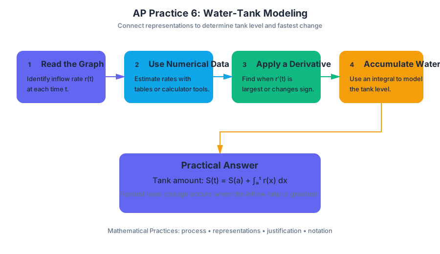
Source Materials
- Learn More (.pdf)
- AP Calculus AB and BC Course and Exam Description
- AP Calculus AB Course Overview
- AP Calculus Course at a Glance
- AP Calculus AB and BC Course at a Glance Poster
- Adopt AP Calculus AB
- AP Calculus AB
- AP Calculus AB
- Figure — AP Calculus AB and BC Course and Exam Description (p. 1)
- Figure — AP Calculus AB and BC Course and Exam Description (p. 14)
- Figure — AP Calculus AB and BC Course and Exam Description (p. 20)
- Figure — AP Calculus AB and BC Course and Exam Description (p. 21)
Study AP Calculus AB with AI — Free on Lykke
Sign up for free to generate personalized flashcards, quizzes, and study guides from this course. Chat with an AI tutor that knows the material.
Get Started FreeView this course wiki on Lykke · Browse all public course wikis