14 01 Principles Of Microeconomics Fall 2018

Supply, Demand, and Market Equilibrium

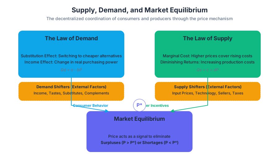
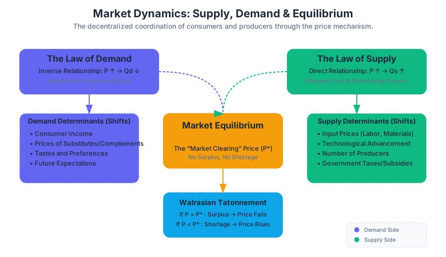
The supply and demand model is the fundamental analytical framework of microeconomics. It functions as a decentralized information-processing system, where prices act as signals that coordinate the independent actions of millions of consumers and producers. Rather than requiring a central planner to allocate resources, the market uses the price mechanism to reach an Equilibrium—a state where the quantity of goods buyers are willing to purchase matches the quantity sellers are willing to provide.

The Law of Demand

The Law of Demand states that, ceteris paribus (all other things being equal), there is an inverse relationship between the price of a good and the quantity demanded. As the price ($P$) increases, the quantity demanded ($Q_d$) decreases.

The Mechanics of Demand

This inverse relationship is driven by two primary economic phenomena:

1. The Substitution Effect: As the price of a good rises, it becomes relatively more expensive compared to other goods. Consumers will naturally pivot toward cheaper substitutes to maintain their utility.
2. The Income Effect: A price increase effectively reduces a consumer's purchasing power. Even if they do not switch to a substitute, they can afford less of the good than before.

Mathematically, a linear demand function is often represented as: $$Q_d = a - bP$$ Where $a$ represents the quantity demanded when price is zero (the horizontal intercept), and $b$ represents the slope of the demand curve (the sensitivity of quantity to price).

Shifts vs. Movements

It is a common pedagogical pitfall to confuse a movement along the demand curve with a shift of the demand curve.

• Movement: Caused solely by a change in the price of the good itself.
• Shift: Caused by a change in external factors (determinants).

Determinant	Effect on Demand Curve	Example
Income (Normal Good)	Increase shifts curve Right	A raise leads to more dining out.
Income (Inferior Good)	Increase shifts curve Left	A raise leads to buying less instant ramen.
Price of Substitutes	Increase shifts curve Right	If coffee prices spike, tea demand rises.
Price of Complements	Increase shifts curve Left	If printer prices spike, ink demand falls.
Tastes/Preferences	Positive change shifts curve Right	A health study praising kale increases demand.
Expectations	Expected future price rise shifts curve Right	Buying gas today because a hike is expected tomorrow.

The Law of Supply

The Law of Supply posits a direct relationship between price and quantity supplied ($Q_s$). As the market price increases, firms are incentivized to produce more because the marginal revenue of selling an additional unit exceeds the marginal cost of production for a larger range of output.

The Marginal Cost Derivation

In a competitive market, a firm's supply curve is essentially its Marginal Cost (MC) curve above the average variable cost. Because of the Law of Diminishing Marginal Returns, producing additional units eventually becomes more expensive (e.g., overtime pay for workers, wear and tear on machinery). Therefore, a higher price is required to justify the higher cost of producing those incremental units.

The linear supply function is typically expressed as: $$Q_s = c + dP$$ Where $c$ is the quantity supplied at a price of zero, and $d$ represents the responsiveness of supply to price changes.

Determinants of Supply

Just as with demand, supply can shift due to external factors:

Factor	Effect on Supply Curve	Technical Reason
Input Prices	Increase shifts curve Left	Higher costs reduce profit margins per unit.
Technology	Improvement shifts curve Right	Increases productivity; lowers marginal cost.
Number of Sellers	Increase shifts curve Right	Aggregate market supply is the sum of individual supplies.
Expectations	Expected future price rise shifts curve Left	Firms may hoard inventory to sell at higher future prices.
Subsidies/Taxes	Subsidy shifts Right; Tax shifts Left	Effectively lowers or raises the cost of production.

Market Equilibrium

Market Equilibrium occurs at the price ($P^*$) where $Q_d = Q_s$. At this point, the market "clears"—there is no excess supply (surplus) and no excess demand (shortage).

The Walrasian Tatonnement

In theory, markets reach equilibrium through a process called tatonnement ("groping"). If the current price is above equilibrium, a surplus exists. Sellers, unable to move their inventory, will lower prices to attract buyers. Conversely, if the price is below equilibrium, a shortage occurs. Buyers, unable to find the product, will bid prices up.

Solving for Equilibrium: A Worked Example

Consider a market with the following functions:

• Demand: $Q_d = 100 - 2P$
• Supply: $Q_s = 20 + 2P$

To find the equilibrium, set $Q_d = Q_s$: $$100 - 2P = 20 + 2P$$ $$80 = 4P$$ $$P^* = 20$$

Substitute $P^$ back into either equation to find $Q^$: $$Q^* = 100 - 2(20) = 60$$

# A simple numerical simulation of market clearing (Walrasian Auctioneer)
def simulate_market_clearing(demand_fn, supply_fn, initial_price, learning_rate=0.1, iterations=50):
    price = initial_price
    history = []

    for i in range(iterations):
        qd = demand_fn(price)
        qs = supply_fn(price)
        excess_demand = qd - qs
        
        history.append({
            "iteration": i,
            "price": round(price, 2),
            "qd": round(qd, 2),
            "qs": round(qs, 2),
            "excess": round(excess_demand, 2)
        })

        # Adjust price based on excess demand
        price += excess_demand * learning_rate
        
        if abs(excess_demand) < 0.01:
            break
            
    return history

# Define functions: Qd = 100 - 2P, Qs = 20 + 2P
demand = lambda p: 100 - 2*p
supply = lambda p: 20 + 2*p

results = simulate_market_clearing(demand, supply, initial_price=40)
for step in results[:5]: # Show first 5 steps
    print(f"P: {step['price']} | Qd: {step['qd']} | Qs: {step['qs']} | Excess: {step['excess']}")

Elasticity

Elasticity measures the responsiveness of one variable to changes in another. While the slope of a curve tells us the absolute change, elasticity provides a percentage-based, unitless measure.

Price Elasticity of Demand (PED)

PED measures how much the quantity demanded responds to a change in price: $$\epsilon_d = \frac{% \Delta Q_d}{% \Delta P}$$

Because demand curves are downward sloping, PED is technically negative, but economists often discuss it in absolute terms.

The Midpoint Method

To avoid different results when calculating elasticity between two points (depending on the direction of the change), the Midpoint Formula is used: $$\epsilon = \frac{(Q_2 - Q_1) / [(Q_2 + Q_1) / 2]}{(P_2 - P_1) / [(P_2 + P_1) / 2]}$$

Classification of Elasticity

| Value of $|\epsilon|$ | Classification | Meaning | | :--- | :--- | :--- | | $|\epsilon| > 1$ | Elastic | Quantity changes more than price (sensitive). | | $|\epsilon| < 1$ | Inelastic | Quantity changes less than price (insensitive). | | $|\epsilon| = 1$ | Unit Elastic | Quantity and price change by the same percentage. | | $|\epsilon| = 0$ | Perfectly Inelastic | Quantity does not change regardless of price (e.g., insulin). | | $|\epsilon| = \infty$ | Perfectly Elastic | Any price increase drops quantity to zero (commodities). |

\text{Derivation of Point Elasticity:} \\
\epsilon = \frac{dQ}{dP} \times \frac{P}{Q} \\
\text{For a demand curve } Q = a - bP, \text{ the derivative } \frac{dQ}{dP} = -b. \\
\text{Thus, } \epsilon = -b \left( \frac{P}{a - bP} \right).

Consumer and Producer Surplus

Equilibrium is not just a point of stability; it is the point that maximizes Total Surplus, the sum of benefits to all market participants.

Consumer Surplus (CS)

Consumer surplus is the difference between what a consumer is willing to pay (their reservation price) and what they actually pay. Graphically, it is the area below the demand curve and above the equilibrium price. $$CS = \int_{0}^{Q^} (P_{demand}(Q) - P^) dQ$$

Producer Surplus (PS)

Producer surplus is the difference between the market price and the marginal cost of production. It represents the benefit to sellers for participating in the market. Graphically, it is the area above the supply curve and below the equilibrium price. $$PS = \int_{0}^{Q^} (P^ - P_{supply}(Q)) dQ$$

Total Surplus and Efficiency

Total Surplus (TS) = CS + PS. An allocation of resources that maximizes total surplus is said to be Pareto Efficient. If a market is prevented from reaching equilibrium (e.g., through a tax or price control), a Deadweight Loss (DWL) occurs—this is surplus that is lost to neither the consumer nor the producer, representing a net loss to society.

-- Example: Calculating Aggregate Consumer Surplus from a Transaction Table
-- Assuming 'orders' table with 'price_paid' and 'max_willingness_to_pay'
SELECT 
    SUM(max_willingness_to_pay - price_paid) AS aggregate_consumer_surplus,
    COUNT(order_id) AS total_transactions,
    AVG(max_willingness_to_pay - price_paid) AS avg_surplus_per_unit
FROM 
    market_orders
WHERE 
    status = 'completed' 
    AND price_paid <= max_willingness_to_pay;

Comparative Statics: Analyzing Market Shocks

Economists use Comparative Statics to predict how equilibrium changes when a determinant shifts. This involves comparing the initial equilibrium to the new equilibrium after a shock.

The Four Laws of Supply and Demand

1. Demand Increases ($\uparrow D$): $P^$ increases, $Q^$ increases.
2. Demand Decreases ($\downarrow D$): $P^$ decreases, $Q^$ decreases.
3. Supply Increases ($\uparrow S$): $P^$ decreases, $Q^$ increases.
4. Supply Decreases ($\downarrow S$): $P^$ increases, $Q^$ decreases.

Ambiguous Cases (Double Shifts)

When both curves shift simultaneously, either the change in price or the change in quantity will be ambiguous unless the magnitudes of the shifts are known.

Shift	$\uparrow$ Supply	$\downarrow$ Supply
$\uparrow$ Demand	$Q \uparrow$, $P$ Ambiguous	$P \uparrow$, $Q$ Ambiguous
$\downarrow$ Demand	$P \downarrow$, $Q$ Ambiguous	$Q \downarrow$, $P$ Ambiguous

Common Pitfalls and Edge Cases

1. The Giffen Good

A rare exception to the Law of Demand where an increase in price causes an increase in quantity demanded. This occurs with highly inferior goods that make up a large portion of a poor consumer's budget. When the price rises, the "income effect" is so negative that the consumer can no longer afford better substitutes (like meat) and must buy more of the staple (like bread or potatoes) to survive.

2. Price Ceilings and Floors

Governments often intervene with price controls.

• Price Ceiling: A legal maximum price (e.g., rent control). If set below equilibrium, it causes a shortage.
• Price Floor: A legal minimum price (e.g., minimum wage). If set above equilibrium, it causes a surplus (unemployment).

3. Tax Incidence

The "burden" of a tax does not depend on who writes the check to the government. Instead, it depends on relative elasticities. The side of the market that is more inelastic (less responsive to price changes) will bear more of the tax burden.

# Simulation Configuration for Market Shock Analysis
simulation_parameters:
  market_name: "Global Semiconductor Market"
  initial_state:
    demand_intercept: 500
    demand_slope: -0.5
    supply_intercept: 50
    supply_slope: 1.2
  shocks:
    - type: "Supply Contraction"
      magnitude: -20%
      reason: "Drought in Taiwan affecting wafer fabrication"
      duration: 12_months
    - type: "Demand Surge"
      magnitude: +15%
      reason: "AI hardware boom"
      duration: 24_months
  metrics_to_track:
    - equilibrium_price
    - equilibrium_quantity
    - deadweight_loss
    - consumer_surplus_delta

Consumer Theory and Firm Behavior

Overview

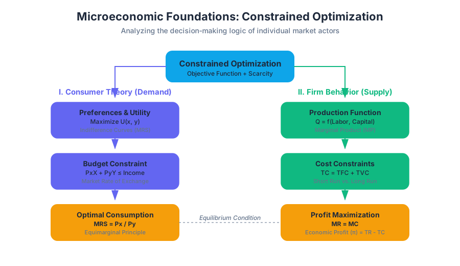
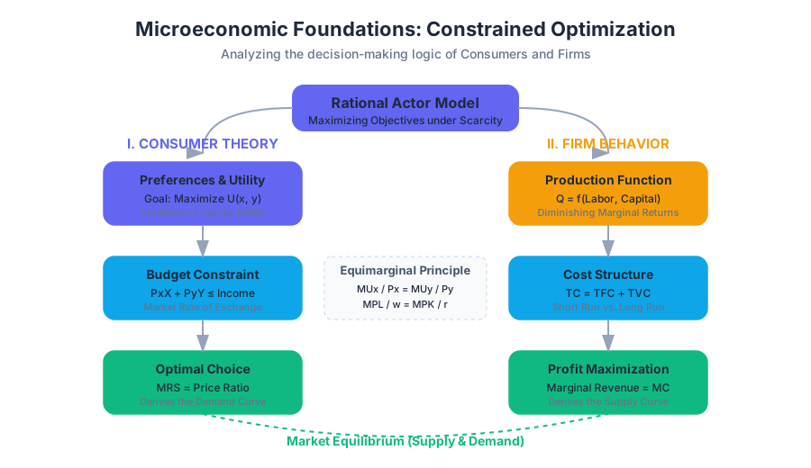
To understand the market, we must first understand the individual actors. This section analyzes the decision-making processes of consumers (the demand side) and firms (the supply side). At its core, microeconomics is the study of constrained optimization: consumers maximize utility subject to a budget, while firms maximize profit subject to technological and market constraints.

---

I. Consumer Theory: The Logic of Choice

Consumer theory seeks to explain how individuals allocate their limited resources across various goods and services. It rests on the assumption of Rationality, meaning consumers have well-defined preferences and act consistently upon them.

1. Preferences and Utility

A consumer’s preferences are represented by a Utility Function, $U(x_1, x_2, ..., x_n)$, which assigns a numerical value to "bundles" of goods. It is important to note that modern economics treats utility as ordinal rather than cardinal; we care about the ranking of bundles, not the specific "utils" assigned to them.

The Axioms of Revealed Preference:

1. Completeness: For any two bundles A and B, a consumer can state $A \succ B$, $B \succ A$, or $A \sim B$.
2. Transitivity: If $A \succ B$ and $B \succ C$, then $A \succ C$.
3. Non-Satiation ("More is Better"): Consumers always prefer more of a good to less.

2. Indifference Curves

An Indifference Curve (IC) represents all combinations of two goods that provide the consumer with the same level of utility.

Property	Description	Economic Implication
Downward Sloping	To keep utility constant, increasing one good requires decreasing the other.	Goods are scarce; trade-offs exist.
Convex to Origin	The curve bows inward toward the (0,0) point.	Diminishing Marginal Rate of Substitution.
Non-Intersecting	Two indifference curves for the same consumer cannot cross.	Logic of transitivity and consistency.
Higher is Better	Curves further from the origin represent higher utility levels.	Non-satiation.

The slope of the indifference curve at any given point is the Marginal Rate of Substitution (MRS). Mathematically, it is the ratio of the marginal utilities: $$MRS_{xy} = -\frac{dU/dx}{dU/dy} = \frac{MU_x}{MU_y}$$

3. The Budget Constraint

Consumers are limited by their income ($I$) and the prices of goods ($P_x, P_y$). The Budget Constraint defines the feasible set of bundles: $$P_x X + P_y Y \leq I$$

The slope of the budget line is $-\frac{P_x}{P_y}$, representing the Market Rate of Exchange or the opportunity cost of consuming good X in terms of good Y.

4. Utility Maximization: The Optimal Choice

The consumer reaches an optimum where the highest possible indifference curve is tangent to the budget line. At this point, the rate at which the consumer is willing to trade goods (MRS) equals the rate at which the market allows them to trade (Price Ratio).

The Lagrangian Derivation: To solve for the optimal bundle $(x^, y^)$, we set up the Lagrangian function: $$\mathcal{L} = U(x, y) + \lambda(I - P_x x - P_y y)$$

Taking first-order conditions (FOC):

1. $\frac{\partial \mathcal{L}}{\partial x} = \frac{\partial U}{\partial x} - \lambda P_x = 0$
2. $\frac{\partial \mathcal{L}}{\partial y} = \frac{\partial U}{\partial y} - \lambda P_y = 0$
3. $\frac{\partial \mathcal{L}}{\partial \lambda} = I - P_x x - P_y y = 0$

Dividing (1) by (2) yields the Equimarginal Principle: $$\frac{MU_x}{P_x} = \frac{MU_y}{P_y}$$ This states that at the optimum, the last dollar spent on each good must yield the same marginal utility.

import numpy as np
from scipy.optimize import minimize

def objective(social_bundle):
    # We want to maximize utility, so we minimize negative utility
    # Example: Cobb-Douglas Utility U = x^0.4 * y^0.6
    x, y = social_bundle
    return -(x**0.4 * y**0.6)

def constraint(social_bundle, income, px, py):
    x, y = social_bundle
    return income - (px * x + py * y)

# Parameters
income_val = 100
price_x = 2
price_y = 5

# Initial guess
x0 = [10, 10]

# Define constraint dictionary
con = {'type': 'eq', 'fun': constraint, 'args': (income_val, price_x, price_y)}

# Optimization
sol = minimize(objective, x0, constraints=con, bounds=[(0, None), (0, None)])

print(f"Optimal x: {sol.x[0]:.2f}")
print(f"Optimal y: {sol.x[1]:.2f}")
print(f"Maximized Utility: {-sol.fun:.2f}")

---

II. Firm Behavior: Production and Costs

While consumers maximize utility, firms maximize Economic Profit ($\pi$), defined as Total Revenue ($TR$) minus Total Cost ($TC$). Unlike accounting profit, economic profit includes Opportunity Costs.

1. The Production Function

The Production Function $Q = f(L, K)$ relates inputs (Labor $L$, Capital $K$) to the maximum output $Q$ possible with current technology.

• Marginal Product (MP): The additional output produced by adding one more unit of an input ($MP_L = \Delta Q / \Delta L$).
• Average Product (AP): Total output divided by the quantity of input ($AP_L = Q / L$).

The Law of Diminishing Marginal Returns: As more of a variable input (like labor) is added to a fixed input (like machinery), the marginal product of the variable input will eventually decline.

2. Short Run vs. Long Run

The distinction is based on the flexibility of inputs:

• Short Run (SR): At least one input (usually Capital) is fixed.
• Long Run (LR): All inputs are variable. Firms can enter/exit the industry and change the scale of production.

Concept	Short Run	Long Run
Fixed Costs	Present (e.g., rent, machinery)	Zero (all costs are variable)
Input Flexibility	Limited adjustment	Full adjustment
Returns to Scale	Not applicable (Diminishing returns)	Constant, Increasing, or Decreasing
Decision Rule	Produce if $P \geq AVC$	Produce if $P \geq ATC$

3. Cost Structures

Total Cost is the sum of Fixed Costs (FC) and Variable Costs (VC).

• Marginal Cost (MC): The cost of producing one additional unit ($MC = dTC/dQ$).
• Average Total Cost (ATC): $TC/Q$.
• Average Variable Cost (AVC): $VC/Q$.

The relationship between these curves is mathematically rigid:

1. When $MC < ATC$, $ATC$ is falling.
2. When $MC > ATC$, $ATC$ is rising.
3. $MC$ intersects $ATC$ and $AVC$ at their respective minimum points.

\text{Derivation of MC and ATC Relationship:} \\
\frac{d}{dQ} \left( \frac{TC(Q)}{Q} \right) = \frac{Q \cdot TC'(Q) - TC(Q)}{Q^2} \\
\text{Set to zero to find the minimum of ATC:} \\
Q \cdot MC - TC = 0 \implies MC = \frac{TC}{Q} \implies MC = ATC

4. Profit Maximization

For any firm, profit is maximized where Marginal Revenue (MR) equals Marginal Cost (MC).

• If $MR > MC$, the firm can increase profit by producing more.
• If $MR < MC$, the firm can increase profit by producing less.

In a Perfectly Competitive market, the firm is a price-taker, so $MR = P$. Thus, the profit-maximizing condition becomes $P = MC$.

---

III. The Link Between Consumer and Firm

The interaction of these two theories creates the market supply and demand curves.

1. From Individual to Market Demand

By varying the price of a good in the consumer's budget constraint and observing the change in the optimal $x^*$, we derive the Price-Consumption Curve. Projecting this onto a Price-Quantity plane yields the individual demand curve. Summing these horizontally across all consumers gives the Market Demand.

2. From Costs to Market Supply

In the short run, a competitive firm's supply curve is the portion of its Marginal Cost curve that lies above the Average Variable Cost (AVC). If the price falls below AVC, the firm minimizes losses by shutting down immediately (the "Shutdown Point").

3. Returns to Scale

In the long run, firms consider how output changes when all inputs are increased proportionally.

Type	Definition	Resulting LRATC Curve
Economies of Scale	Output more than doubles when inputs double.	Downward sloping
Constant Returns	Output exactly doubles when inputs double.	Flat / Horizontal
Diseconomies of Scale	Output less than doubles when inputs double.	Upward sloping

-- Example: Analytical query for a firm to calculate Marginal Cost 
-- from a production log table.

WITH CostCalculations AS (
    SELECT 
        batch_id,
        total_output_units,
        total_variable_cost,
        total_fixed_cost,
        (total_variable_cost + total_fixed_cost) AS total_cost,
        LAG(total_output_units) OVER (ORDER BY batch_id) as prev_output,
        LAG(total_variable_cost + total_fixed_cost) OVER (ORDER BY batch_id) as prev_total_cost
    FROM production_logs
)
SELECT 
    batch_id,
    total_output_units,
    total_cost / total_output_units AS average_total_cost,
    (total_cost - prev_total_cost) / NULLIF(total_output_units - prev_output, 0) AS marginal_cost
FROM CostCalculations;

---

IV. Common Pitfalls and Advanced Nuances

1. The Giffen Good Paradox

While the Law of Demand states that demand curves slope downward, Giffen Goods are a theoretical exception. For these goods, an increase in price leads to an increase in quantity demanded because the negative Income Effect outweighs the Substitution Effect. This typically only happens with extreme inferior goods that consume a large portion of a consumer's budget.

2. Sunk Cost Fallacy in Firm Behavior

Firms (and students) often mistakenly include Sunk Costs (costs already incurred and unrecoverable) in their decision-making. Rational firms ignore sunk costs and only consider Prospective Costs. Fixed costs are sunk in the short run, which is why a firm will continue to operate even at a loss, provided it covers its variable costs.

3. Technical vs. Economic Efficiency

A production process is technically efficient if it minimizes inputs for a given output. It is economically efficient if it minimizes costs. A firm might be technically efficient but economically inefficient if it uses an expensive input where a cheaper substitute exists.

Market Structures and Competition

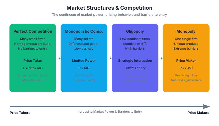
In neoclassical microeconomics, the behavior of a firm is not dictated solely by its internal production function, but by the external environment in which it operates. This environment, known as the Market Structure, determines the degree of pricing power a firm possesses, the barriers to entry for potential competitors, and the ultimate efficiency of resource allocation.

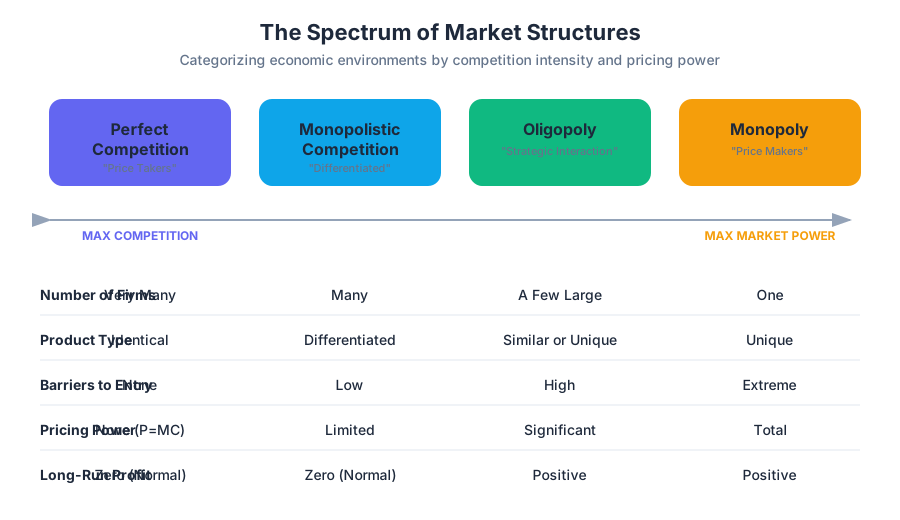
At one end of the spectrum lies Perfect Competition, a theoretical benchmark where firms are "price takers." At the other lies Monopoly, where a single firm wields total market power. Between these extremes are Oligopoly and Monopolistic Competition, where strategic interactions and product differentiation define the landscape. Understanding these structures requires a rigorous application of marginal analysis and, in the case of strategic interaction, Game Theory.

Perfect Competition

Perfect competition represents an idealized market state where the forces of supply and demand operate without friction. It serves as the baseline against which all other market "imperfections" are measured.

1. Characteristics and Assumptions

For a market to be considered perfectly competitive, four stringent criteria must be met:

• Large Number of Buyers and Sellers: No individual agent has a large enough market share to influence the equilibrium price.
• Homogeneous Products: The goods offered by different sellers are perfect substitutes. Consumers are indifferent between sellers.
• Perfect Information: All agents have complete knowledge of prices, technologies, and profit opportunities.
• Free Entry and Exit: There are no legal, technological, or financial barriers preventing firms from entering or leaving the industry in the long run.

2. The Firm's Decision: Price Taking

In this structure, the firm faces a perfectly elastic demand curve at the market price $P^*$. The firm's total revenue is $TR = P \cdot Q$, and because $P$ is constant, the Marginal Revenue (MR) is simply $P$.

The Profit Maximization Rule: To maximize profit $\pi$, a firm must produce at the quantity $Q$ where the cost of the last unit produced equals the revenue it generates: $$P = MC(Q)$$

3. Long-Run Equilibrium and the Zero-Profit Condition

In the short run, a firm may earn economic profits if $P > ATC$ (Average Total Cost). However, these profits signal an opportunity to outsiders. Due to the assumption of free entry, new firms will enter the market, shifting the industry supply curve to the right and driving down the price. This process continues until $P = \min(ATC)$, at which point Economic Profit is zero.

Parameter	Short Run	Long Run
Profit ($\pi$)	Can be positive, zero, or negative	Must be zero (Normal Profit)
Price (P)	$P = MC$	$P = MC = \min(ATC)$
Efficiency	Allocative efficiency achieved	Allocative and Productive efficiency achieved
Firm Behavior	Adjusts $Q$ to $P$	Enters/Exits based on $\pi$

4. Implementation: Simulating Market Convergence

The following Python script simulates a perfectly competitive market where firms enter based on profit signals, eventually driving the market toward a zero-profit equilibrium.

import numpy as np

class CompetitiveMarket:
    def __init__(self, initial_price, cost_function_params):
        self.price = initial_price
        self.firms = 10  # Starting number of firms
        self.a, self.b = cost_function_params # TC = a*Q^2 + b*Q
        
    def firm_supply(self, price):
        # P = MC => P = 2*a*Q + b => Q = (P - b) / (2*a)
        return max(0, (price - self.b) / (2 * self.a))

    def market_supply(self):
        return self.firms * self.firm_supply(self.price)

    def market_demand(self, price):
        # Simple linear demand: Qd = 1000 - 50P
        return max(0, 1000 - 50 * price)

    def step(self, learning_rate=0.1):
        # Calculate equilibrium price for current number of firms
        # Qd = Qs => 1000 - 50P = N * (P - b) / (2a)
        # 1000 + (N*b)/(2a) = P * (50 + N/(2a))
        numerator = 1000 + (self.firms * self.b) / (2 * self.a)
        denominator = 50 + (self.firms / (2 * self.a))
        self.price = numerator / denominator
        
        # Calculate profit per firm: pi = P*q - (a*q^2 + b*q)
        q = self.firm_supply(self.price)
        profit = (self.price * q) - (self.a * q**2 + self.b * q)
        
        # Entry/Exit logic
        if profit > 0.5:
            self.firms += 1
        elif profit < -0.5 and self.firms > 1:
            self.firms -= 1
            
        return self.price, self.firms, profit

# Simulation execution
market = CompetitiveMarket(initial_price=20, cost_function_params=(0.5, 2))
for i in range(50):
    p, n, pi = market.step()
    if i % 10 == 0:
        print(f"Iteration {i}: Price={p:.2f}, Firms={n}, Profit={pi:.2f}")

Monopoly

A Monopoly exists when a single firm is the sole producer of a product with no close substitutes. Unlike the competitive firm, the monopolist is a "price maker."

1. Barriers to Entry

Monopolies persist only if other firms are prevented from entering. These barriers include:

• Ownership of Key Resources: (e.g., De Beers and diamonds).
• Government Franchises/Patents: Legal protections for intellectual property.
• Natural Monopolies: Occur when Economies of Scale are so significant that a single firm can supply the entire market at a lower cost than two or more firms could (e.g., water utilities).

2. The Math of Monopoly Power

The monopolist faces the downward-sloping market demand curve $P(Q)$. Consequently, to sell an additional unit, the firm must lower the price on all units sold. This implies that Marginal Revenue (MR) is always less than Price ($P$).

Derivation of Marginal Revenue: Let $TR = P(Q) \cdot Q$. $MR = \frac{d(TR)}{dQ} = P + Q \cdot \frac{dP}{dQ}$ Since $\frac{dP}{dQ} < 0$ for a downward sloping demand curve, $MR < P$.

3. The Lerner Index

The degree of monopoly power is often measured by the Lerner Index ($L$), which quantifies the markup over marginal cost.

L = \frac{P - MC}{P} = \frac{1}{|\epsilon_d|}

Where $\epsilon_d$ is the price elasticity of demand. This formula demonstrates that the less elastic the demand (smaller $\epsilon_d$), the greater the firm's ability to charge a price significantly above marginal cost.

4. Social Cost: Deadweight Loss

Monopolies are inefficient because they produce a quantity where $P > MC$. This results in Deadweight Loss (DWL)—a loss of total surplus (consumer + producer) that occurs because the firm restricts output to keep prices high.

Feature	Perfect Competition	Monopoly
Quantity	$Q_{comp}$ where $P = MC$	$Q_{mono}$ where $MR = MC$
Price	$P = MC$	$P > MC$
Welfare	Maximizes Total Surplus	Creates Deadweight Loss
Long-run Profit	Zero	Can be positive

Oligopoly

An Oligopoly is a market structure dominated by a small number of large firms. The defining characteristic of an oligopoly is Strategic Interdependence: the profit of one firm depends not only on its own actions but also on the actions of its rivals.

1. The Cournot Model (Quantity Competition)

In the Cournot model, firms simultaneously choose the quantity they will produce. Each firm treats the other's output as fixed. The equilibrium occurs at the intersection of the firms' Reaction Functions.

2. The Bertrand Model (Price Competition)

In the Bertrand model, firms compete on price. If products are homogeneous, consumers will always buy from the firm with the lowest price. This leads to a "race to the bottom" where $P = MC$, even with only two firms. This is known as the Bertrand Paradox.

3. Measuring Market Concentration: HHI

Regulators use the Herfindahl-Hirschman Index (HHI) to determine the competitiveness of an industry. It is calculated by squaring the market share of each firm.

-- SQL query to calculate HHI for a market based on firm sales
WITH MarketSales AS (
    SELECT 
        firm_id, 
        SUM(revenue) as firm_revenue
    FROM sales_data
    GROUP BY firm_id
),
TotalMarket AS (
    SELECT SUM(firm_revenue) as total_revenue FROM MarketSales
),
Shares AS (
    SELECT 
        (firm_revenue / (SELECT total_revenue FROM TotalMarket)) * 100 as market_share
    FROM MarketSales
)
SELECT 
    SUM(market_share * market_share) as HHI
FROM Shares;

• HHI < 1,500: Unconcentrated (Competitive).
• 1,500 < HHI < 2,500: Moderately Concentrated.
• HHI > 2,500: Highly Concentrated (Oligopolistic).

Game Theory and Nash Equilibrium

Because oligopolists must act strategically, we use Game Theory to model their behavior.

1. Components of a Game

A game consists of:

1. Players: The decision-makers (firms).
2. Strategies: The possible actions (e.g., High Price, Low Price).
3. Payoffs: The outcomes (profits) resulting from the combination of strategies.

2. Nash Equilibrium

A Nash Equilibrium is a situation where each player chooses their best strategy, given the strategies chosen by the other players. No player has an incentive to deviate unilaterally.

Formal Definition: A strategy profile $(s^_i, s^{-i})$ is a Nash Equilibrium if for every player $i$: $$\pi_i(s^_i, s^{-i}) \geq \pi_i(s_i, s^*_{-i}) \quad \forall s_i \in S_i$$

3. The Prisoner's Dilemma in Business

Oligopolies often face a Prisoner's Dilemma. While both firms would earn higher profits by colluding (forming a Cartel) and keeping prices high, the individual incentive to "cheat" by lowering prices to capture the whole market often leads to a sub-optimal equilibrium for the firms.

Firm A \ Firm B	Collude (High P)	Cheat (Low P)
Collude (High P)	($10M, $10M)	($2M, $15M)
Cheat (Low P)	($15M, $2M)	($5M, $5M)

In this matrix, (Cheat, Cheat) is the Nash Equilibrium, even though (Collude, Collude) yields higher collective profits.

4. Repeated Games and Tit-for-Tat

In the real world, firms interact repeatedly. This allows for the development of "trigger strategies." In a Tit-for-Tat strategy, a firm cooperates in the first period and subsequently mimics the rival's previous move. This can sustain collusion without an explicit (and illegal) agreement.

Summary of Market Structures

Feature	Perfect Competition	Monopolistic Competition	Oligopoly	Monopoly
Number of Firms	Many	Many	Few	One
Type of Product	Identical	Differentiated	Identical or Differentiated	Unique
Barriers to Entry	None	Low	High	Very High
Pricing Power	None (Price Taker)	Some	Substantial	Total (Price Maker)
Example	Wheat, Stocks	Restaurants, Clothing	Airlines, Soft Drinks	Local Utilities

Common Pitfalls and Misconceptions

1. "Monopolies can charge any price they want": False. Monopolists are still constrained by the demand curve. If they set the price too high, the quantity demanded drops to zero. They set the price to maximize $\pi$, not to maximize $P$.
2. "Zero economic profit means the firm is failing": False. Economic profit includes Opportunity Cost. Zero economic profit means the firm's owners are earning exactly what they could have earned in their next best alternative (a "normal" return on investment).
3. "Nash Equilibrium is always the best outcome": False. As seen in the Prisoner's Dilemma, the Nash Equilibrium is often Pareto-inefficient, meaning there is another outcome where at least one player is better off without making anyone else worse off.

Welfare Economics and Public Policy

Welfare economics is the normative branch of economics that evaluates the well-being of society as a whole. While microeconomics often focuses on how individual agents (firms and consumers) maximize their own utility or profit, welfare economics asks a higher-order question: Under what conditions does the pursuit of individual self-interest lead to a socially optimal outcome?

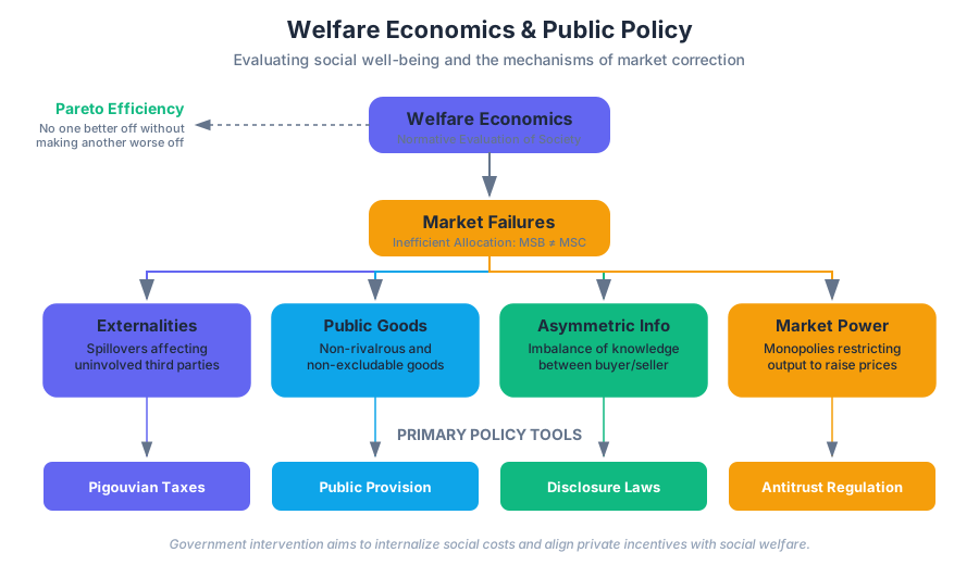
The foundational pillars of this field are the First and Second Fundamental Theorems of Welfare Economics. The First Theorem states that under certain idealized conditions (perfect competition, no externalities, symmetric information), a competitive equilibrium is Pareto Efficient—meaning no one can be made better off without making someone else worse off. However, in the real world, these conditions are rarely met. These deviations are known as Market Failures, and they provide the primary justification for government intervention through public policy.

The Framework of Market Failure

A market failure occurs when the price mechanism fails to account for all costs and benefits associated with a transaction. This results in an inefficient allocation of resources, where the marginal social benefit (MSB) does not equal the marginal social cost (MSC).

Failure Type	Description	Primary Policy Tool
Externalities	Spillovers affecting third parties not involved in the transaction.	Pigouvian Taxes / Subsidies
Public Goods	Goods that are non-rivalrous and non-excludable.	Public Provision / Taxation
Asymmetric Information	One party has superior information, leading to market collapse.	Regulation / Disclosure Laws
Market Power	Monopolies or oligopolies restricting output to raise prices.	Antitrust Laws / Price Caps

---

Externalities: The Divergence of Private and Social Costs

An externality occurs when the production or consumption of a good imposes an unintended cost or benefit on a third party. Because these "spillovers" are not reflected in market prices, the equilibrium quantity ($Q_{mkt}$) deviates from the socially optimal quantity ($Q_{opt}$).

Negative Externalities and Pigouvian Taxes

In the case of pollution (a negative externality), the Marginal Private Cost (MPC) of a firm is lower than the Marginal Social Cost (MSC). The MSC is the sum of the MPC and the Marginal External Cost (MEC).

The Social Optimality Condition: $MSC = MPC + MEC = MSB$

To correct this, economists propose a Pigouvian Tax—a tax set exactly equal to the MEC at the optimal level of output. This "internalizes" the externality, forcing the firm to treat the social cost as a private cost.

The Coase Theorem

Coase argued that if transaction costs are zero and property rights are well-defined, private parties can bargain to reach the efficient outcome regardless of who holds the initial property rights. However, in practice, transaction costs (legal fees, coordination issues) often prevent this, necessitating government intervention.

Implementation: Numerical Optimization of Pigouvian Taxes

The following Python implementation demonstrates how to find the optimal tax rate for a firm with a quadratic cost function and a linear damage function (negative externality).

import numpy as np
from scipy.optimize import minimize_scalar

def solve_optimal_tax():
    """
    Calculates the Pigouvian tax required to align private 
    production with social welfare.
    
    Demand (MSB): P = 100 - Q
    Private Cost (MPC): 10 + 2Q
    External Damage (MEC): 0.5 * Q^2 (Total damage), so MEC = Q
    """
    
    # 1. Private Equilibrium (MPC = MSB)
    # 10 + 2Q = 100 - Q  => 3Q = 90 => Q = 30
    q_mkt = 30
    
    # 2. Social Optimum (MSC = MSB)
    # MSC = MPC + MEC = (10 + 2Q) + Q = 10 + 3Q
    # 10 + 3Q = 100 - Q => 4Q = 90 => Q = 22.5
    q_opt = 22.5
    
    # 3. The Pigouvian Tax (t = MEC at Q_opt)
    # MEC = Q, so at Q_opt = 22.5, t = 22.5
    tax_rate = q_opt
    
    return {
        "Market Quantity": q_mkt,
        "Socially Optimal Quantity": q_opt,
        "Optimal Pigouvian Tax": tax_rate
    }

results = solve_optimal_tax()
for key, value in results.items():
    print(f"{key}: {value}")

---

Public Goods and the Free Rider Problem

Public goods are defined by two technical characteristics:

1. Non-rivalry: One person’s consumption does not reduce the amount available to others.
2. Non-excludability: It is impossible (or prohibitively expensive) to prevent non-payers from consuming the good.

The Samuelson Condition

For private goods, we sum individual demand curves horizontally (adding quantities at each price). For public goods, we sum them vertically (adding the marginal willingness to pay at each quantity). The optimal provision of a public good is reached when the sum of individual marginal benefits equals the marginal cost of production.

\sum_{i=1}^{n} MRS_i = MRT

Where $MRS$ is the Marginal Rate of Substitution (individual benefit) and $MRT$ is the Marginal Rate of Transformation (social cost).

The Tragedy of the Commons

This is a specific subset of public goods (Common Pool Resources) that are rivalrous but non-excludable (e.g., fisheries). Because users do not pay for the depletion of the resource, they over-exploit it, leading to total collapse.

Good Category	Rivalrous	Non-Rivalrous
Excludable	Private Goods (Food, Clothing)	Club Goods (Netflix, Gyms)
Non-Excludable	Common Resources (Fish stocks)	Public Goods (Defense, Air)

---

Asymmetric Information: Lemons, Signaling, and Moral Hazard

Market failure often stems from an imbalance of information. This manifests in two primary ways: Adverse Selection (hidden characteristics) and Moral Hazard (hidden actions).

Adverse Selection (The Lemons Problem)

George Akerlof demonstrated that if buyers cannot distinguish between high-quality ("peaches") and low-quality ("lemons") used cars, they will only offer a price reflecting the average quality. High-quality sellers will exit the market, further lowering the average quality, until the market potentially collapses.

Mathematical Derivation of Market Collapse

Consider a market where quality $\theta$ is uniformly distributed between 0 and 1. Sellers value their car at $\theta$, and buyers value it at $1.5\theta$.

1. If buyers cannot observe theta, they assume E[theta] = 0.5.
2. Buyers offer Price P = 1.5 * E[theta | seller accepts].
3. A seller accepts if theta <= P.
4. If P is offered, the average quality of cars sold is E[theta | theta <= P] = P/2.
5. Equilibrium requires P = 1.5 * (P/2) = 0.75P.
6. This equation only holds if P = 0.
7. Result: The market for high-quality goods collapses entirely.

Moral Hazard

Moral hazard occurs after a contract is signed. For example, an insured person may take more risks because they do not bear the full cost of a negative outcome. This is why insurance companies use deductibles and co-pays to re-align incentives.

---

Taxation and Deadweight Loss

Governments must raise revenue to provide public goods and correct externalities. However, taxes (except for Pigouvian taxes) generally create a Deadweight Loss (DWL) by driving a wedge between the price buyers pay and the price sellers receive.

The Harberger Triangle

The DWL is represented by a triangle in the supply-demand framework. Its size is proportional to the square of the tax rate and the elasticities of supply and demand.

DWL Formula (Approximation): $DWL = 0.5 \times \epsilon \times P \times Q \times \tau^2$ Where $\epsilon$ is the elasticity and $\tau$ is the tax rate.

Optimal Taxation (The Ramsey Rule)

To minimize total DWL across a whole economy, the government should tax goods with inelastic demand more heavily. This is because consumers of inelastic goods (like insulin or salt) do not change their behavior significantly in response to price changes, minimizing the "wedge" effect.

Elasticity Condition	Tax Burden (Incidence)	Efficiency Impact
Inelastic Demand	Consumers bear most of the tax.	Low Deadweight Loss.
Elastic Demand	Producers bear most of the tax.	High Deadweight Loss.
Inelastic Supply	Producers bear most of the tax.	Low Deadweight Loss.

Policy Implementation: Tracking Tax Compliance

In a modern digital economy, taxation policy is often implemented via automated systems. Below is a SQL schema for a "Value Added Tax" (VAT) tracking system used to ensure transparency and reduce information asymmetry.

-- Schema for a Policy-Compliant VAT Tracking System
CREATE TABLE products (
    product_id SERIAL PRIMARY KEY,
    name VARCHAR(255),
    category VARCHAR(50), -- e.g., 'Luxury', 'Essential'
    base_price DECIMAL(10, 2)
);

CREATE TABLE tax_rates (
    category VARCHAR(50) PRIMARY KEY,
    rate_percent DECIMAL(5, 2) -- Ramsey Rule: Essentials < Luxury
);

CREATE TABLE transactions (
    tx_id UUID PRIMARY KEY,
    product_id INT REFERENCES products(product_id),
    seller_id INT,
    buyer_id INT,
    sale_price DECIMAL(10, 2),
    tax_collected DECIMAL(10, 2) GENERATED ALWAYS AS (
        sale_price * (SELECT rate_percent FROM tax_rates r 
                      JOIN products p ON p.category = r.category 
                      WHERE p.product_id = transactions.product_id) / 100
    ) STORED
);

---

Social Welfare Functions: How to Aggregate Well-being

Even if a policy is efficient, is it "fair"? Welfare economics uses Social Welfare Functions (SWF) to aggregate individual utilities ($U_i$) into a single measure of social well-being ($W$).

1. Utilitarian (Benthamite): $W = \sum U_i$. The goal is to maximize the total sum of utility, regardless of distribution.
2. Rawlsian (Maximin): $W = \min(U_1, U_2, \dots, U_n)$. Social welfare is only as high as the utility of the least well-off member. This justifies significant redistribution.
3. Bergson-Samuelson: A generalized form where $W = f(U_1, U_2, \dots, U_n)$, allowing for different weights on different individuals.

Comparison of Welfare Philosophies

Philosophy	Objective	Policy Implication
Pareto	No one worse off	Only "win-win" moves allowed.
Utilitarian	Maximize total $U$	Redistribute if $MU$ of poor > $MU$ of rich.
Rawlsian	Maximize $U_{min}$	Heavy safety nets and progressive taxes.
Kaldor-Hicks	Winners can compensate losers	Efficiency-focused; compensation is theoretical.

---

Common Pitfalls in Public Policy Analysis

1. Ignoring General Equilibrium Effects: A tax on plastic bags might increase the use of paper bags, which have a higher carbon footprint to produce. Policy must look beyond the immediate market.
2. The "Nirvana Fallacy": Comparing a "failed" market to an "ideal" government. Governments also face failures (rent-seeking, bureaucracy, and lack of information).
3. Confusing Equity with Efficiency: A policy can be perfectly efficient (no DWL) but highly inequitable (all wealth goes to one person). Welfare economics requires balancing both.
4. Tax Salience: Assuming consumers respond to taxes the same way they respond to price changes. Behavioral economics shows that "hidden" taxes (like those included in the price) have different effects than taxes added at the register.

Real-World CLI: Accessing Economic Data

Economists often use APIs to pull real-world data for welfare analysis. Here is a sample curl command to fetch CPI data (inflation) from the Federal Reserve Economic Data (FRED) API, which is crucial for adjusting welfare measures over time.

# Fetch Consumer Price Index (CPI) data for welfare adjustment
curl -X GET "https://api.stlouisfed.org/fred/series/observations?series_id=CPIAUCSL&api_key=YOUR_API_KEY&file_type=json" \
     -H "Accept: application/json" | jq '.observations[-1]'